Big Model Strategy for Bridge Structural Health Monitoring Based on Data-Driven, Adaptive Method and Convolutional Neural Network (CNN) Group

1  Introduction

Structural Health Monitoring (SHM) plays a pivotal role in ensuring the safety and longevity of bridges by providing real-time insights into their structural condition [1]. By continuously monitoring various parameters such as vibrations, strain, and environmental factors, SHM enables early detection of potential issues, facilitating timely maintenance and intervention. The significance lies in enhancing public safety, optimizing maintenance practices, and prolonging the lifespan of critical infrastructure [2]. However, analyzing large-scale structural data poses challenges such as data complexity, integration of diverse sensor outputs, and the need for advanced analytical methods. Handling vast datasets from numerous sensors requires robust algorithms, computational resources, and expertise to extract meaningful patterns and make informed decisions for optimal bridge management and resilience. The “Big Model” strategy, within the context of bridge data analysis, involves deploying complex and highly sophisticated models, particularly Convolutional Neural Networks (CNN) groups, to handle the intricacies of large and diverse datasets. This approach aims to capture nuanced patterns and correlations within complex structural health monitoring data from bridges. CNNs, renowned for their effectiveness in image and sequence analysis, are organized into groups to collectively process various aspects of the data, such as vibration patterns, strain measurements, and environmental influences. The “Big Model” strategy is relevant in addressing the multifaceted challenges posed by the sheer volume and complexity of bridge data. The contribution of this work represents in integrating Finite Element Analysis, time-frequency analysis, and Convolutional Neural Networks to enhance Bridge Structural Health Monitoring. It utilizes comprehensive data from diverse sensors, sophisticated feature extraction, and advanced CNN architecture, optimizing performance through rigorous preprocessing and hyperparameter tuning. Also, this strategy enables the extraction of intricate features, enhancing the model’s ability to make accurate predictions, monitor structural health, and contribute to proactive maintenance practices for resilient and safe infrastructure.

2  Background

Existing methods for Structural Health Monitoring (SHM) encompass a range of techniques, from traditional sensor-based approaches to advanced data-driven methodologies [3,4]. Traditional methods include strain gauges, accelerometers, and visual inspections, providing valuable but often discrete and localized information. Additionally, Finite Element Analysis (FEA) and model-based approaches offer insights into structural behavior but may lack real-time adaptability. Traditional methods often handle specific data types in isolation, making it challenging to integrate diverse sensor outputs. Traditional methods may struggle to analyze large-scale datasets generated by numerous sensors. Traditional methods may face challenges in identifying complex patterns indicative of structural degradation. Many traditional methods are static and may not adapt well to evolving environmental or operational conditions. It notes that while SHM can significantly enhance the lifespan of structures and improve public safety, technical and environmental factors can impact the accuracy of SHM data [5]. Conventional techniques in structural health monitoring (SHM) often exhibit specialization towards particular bridge designs or environmental conditions. When focusing on the initial level of SHM assessment, which involves detection, the methods described in existing literature typically fall into two main categories: data-driven approaches and model-based approaches [6]. Data-driven methods operate by discerning damage-sensitive characteristics from collected data without necessarily relying on a predefined physics-based system model [7,8]. Conversely, model-based methods presuppose the existence of a system model, frequently numerical in nature (such as finite-element-based models), which is frequently updated to align with the observed measurements [9]. For the detection phase, purely data-driven methods often demonstrate high efficiency. However, their lack of direct physical interpretation can impede more advanced tasks within the SHM framework, such as quantification and localization. Model-based techniques are better suited to address these advanced tasks, leveraging the structural system model, but they often entail substantially higher computational demands, posing challenges for real-time applications like diagnostics and control. Hybrid approaches represent a middle ground, integrating finite element information into data-driven methodologies. This fusion aims to produce damage indicators that harness the advantages of model-based features without necessitating extensive model updating [10]. Moreover, data-driven methods can be further classified based on the signal processing tools they utilize, as outlined in studies such as [11,12].

However, these methods frequently encounter ill-posed challenges arising from environmental disturbances inherent in outdoor civil structures, including light variations, distortion, weather conditions, shading, and occlusion [13]. In response, the SHM community has increasingly turned to innovative solutions leveraging computer vision and artificial intelligence (AI) techniques, which exhibit diminished sensitivity to external disruptions and offer superior feature selection capabilities. Salehi et al. [14] conducted an inclusive review of various AI methodologies used in structural engineering, highlighting a recent shift towards AI-supported research emphasizing pattern recognition and machine learning-based automated data-driven approaches. The authors critically examined the strengths and limitations of diverse AI techniques within various structural engineering contexts. Ying et al. [15] conducted a comprehensive review of machine learning (ML)-based SHM algorithms tailored for detecting damage in steel pipes amidst varying environmental conditions. Building upon this, Feng et al. [16] contributed an exhaustive literature review focusing on cutting-edge computer vision techniques utilizing vision-based displacement sensors for SHM applications. The majority of these methods relied on template matching algorithms to extract displacement time-histories from video and image data. Challenges associated with extracting displacement information from both 2D and 3D measurements, and from diverse artificial or natural targets, were thoroughly discussed, alongside considerations for real-time implementation and preprocessing procedures. Also, Gomes et al. [17] offered an extensive examination of intelligent computational tools available for damage detection and system identification, with specific emphasis on composite structures. Addressing the latest advancements, Spencer et al. [18] provided insights into state-of-the-art vision-based techniques for structural condition assessment, incorporating computer vision and ML algorithms. Challenges pertaining to both static and dynamic measurement techniques were deliberated upon, alongside envisaged future directions emphasizing automated decision-making enhancements for SHM.

Martucci et al. [19] stated that SHM is crucial in civil, mechanical, and aerospace engineering for identifying and assessing damage using modal parameters. They highlight the efficiency of output-only techniques, or operational modal analysis (OMA), for large structures and propose automating OMA with machine learning, specifically through a novel multi-stage clustering algorithm. This approach is tested on a scaled masonry arch bridge model to detect and assess damage severity. While Civera et al. [20] stated that the Extreme Function Theory (EFT) combined with Gaussian Process Regression (GPR) offers an efficient, automated tool for mode shape-based damage detection in SHM. This method reduces false positive errors and has been validated experimentally on the I-40 bridge, showing its effectiveness for monitoring large civil structures and infrastructures.

Ahmadi et al. [21] presented a novel algorithm based on square time-frequency distribution (TFD) for detecting damage in concrete piers of railroad bridges. The algorithm, corroborated using a finite element model of the Qotour railroad bridge, utilizes two new damage indices and extensive in situ measurements and lab tests. It accurately identifies damage severity, is noise-resistant, and only requires response signals, eliminating the need for recording excitation forces or creating an analytical model, which is particularly useful for complex bridge structures. Also, Ahmadi et al. [22] emphasized the importance of early damage identification for preserving structures and preventing worsening conditions. They present a novel algorithm for detecting damage in steel girders of bridge decks using Bern-Jordan TFD and a proposed damage index (C-Index). Evaluated on the College Bridge with 10 different damage scenarios, the algorithm accurately identifies damage locations, showing its effectiveness in monitoring structural integrity.

Zha et al. [23] stated that vision-based structural health monitoring (SHM) using deep convolutional neural networks (CNNs), specifically deep residual neural networks, has shown significant promise for recognizing and evaluating structural damage post-natural disasters. Using transfer learning and a dataset from the 2018 PEER Hub ImageNet Challenge, they tackled eight structural damage detection tasks, achieving classification accuracy between 63.1% and 99.4%, and secured third place overall. They noted that improving training data precision could further enhance accuracy. While Gao et al. [24] stated that structural health monitoring of bridges is crucial for post-earthquake recovery, and integrating machine learning enhances damage detection. This study used time-series data from shake-table experiments on a two-span bridge, converting it into images for convolutional neural network (CNN) analysis. CNN models trained on Markov transition field encoded images from acceleration data achieved 100% accuracy during training and over 94% in testing. Overall, the literature suggests that ML methods heavily rely on robust feature extraction, often followed by the application of appropriate classifiers. Mantawy et al. [25] proposed a deep neural network (DNN)-based SHM method for real-time crack detection and localization using a small number of strain gauge sensors. By combining DNN with principal component analysis (PCA), the method predicts the strain field from sparsely located sensors, confirmed through cyclic 4-point bending tests on composite material specimens. The technique accurately predicted the strain field for all specimens considered. While these techniques demonstrate efficacy in managing small anomaly datasets, their applicability may be limited in the context of large-scale civil structures like buildings, bridges, dams, pipelines, and wind turbines, where crack patterns tend to exhibit complex and irregular characteristics [26].

3  Methodology

The proposed methodology employs a comprehensive approach for Bridge Structural Health Monitoring (SHM) by integrating Finite Element Analysis (FEA), time-frequency analysis, and a Convolutional Neural Network (CNN). Initial data collection encompasses information from diverse bridge sensors, covering strain gauges, accelerometers, and other relevant instruments, capturing a range of operational and environmental conditions. FEA is utilized to simulate structural behavior, extracting critical features. Concurrently, time-frequency analysis techniques are applied to sensor data for capturing time-varying characteristics. The integrated dataset, comprising both simulated and real-world responses, is then processed by a CNN. This architecture, featuring multiple CNNs organized to focus on specific aspects of the data, is trained on labeled datasets representing various health states. The trained model is validated, and its performance assessed using metrics, providing insights into structure health. Continuous monitoring, maintenance planning, and iterative improvements ensure the method’s adaptability to evolving conditions and its effectiveness in enhancing bridge safety and longevity.

In optimizing the effectiveness of the proposed Big Model Strategy for Bridge Structural Health Monitoring, several preprocessing steps and considerations were employed. Data normalization played a crucial role in ensuring uniform scales across diverse sensor inputs, preventing biased learning. Feature engineering encompassed the extraction of pertinent information from both Finite Element Analysis (FEA) and time-frequency analyses, augmenting the dataset with meaningful features relevant to structural health. Missing data points were addressed through careful imputation strategies, preserving data integrity. Extensive hyperparameter tuning involved systematic adjustments to the CNN architecture, with considerations for learning rates, filter sizes, and dropout rates. Regularization techniques, including dropout layers, were implemented to mitigate overfitting risks, promoting better generalization to real-world scenarios. Model architecture considerations were refined through iterative experimentation, exploring various layer configurations and ensemble methods to optimize predictive accuracy. Learning rate scheduling contributed to the stability of the training process, while cross-validation techniques provided a comprehensive assessment of model generalization across diverse subsets of the dataset. Interpretability analyses were incorporated to enhance collaboration with domain experts, fostering transparency and trust in the model’s decision-making process. These meticulous preprocessing steps and considerations collectively contributed to the model’s effectiveness in accurately predicting structural health and anomalies in bridge structures.

3.1 Convolutional Neural Networks (CNN)

Convolutional Neural Networks (CNNs) are designed with a hierarchical and layered architecture that has proven exceptionally effective in image-based data analysis. Consisting of convolutional layers that scan input images with learnable filters, pooling layers for spatial dimension reduction, activation layers for introducing non-linearities, and fully connected layers for global feature aggregation, CNNs excel in capturing intricate patterns and hierarchical representations within images. Their applications in image-based data analysis are diverse, encompassing image classification, object detection, and segmentation. CNNs are extensively used for tasks such as facial recognition, medical image analysis, and artistic style transfer. Their ability to automatically learn features and relationships in large datasets makes CNNs a cornerstone in computer vision, contributing to advancements in various fields requiring sophisticated image processing and pattern recognition capabilities. CNNs demonstrate remarkable suitability for processing structural data, particularly in the context of Structural Health Monitoring (SHM), due to their innate capacity to capture intricate patterns within large datasets. The hierarchical architecture of CNNs aligns well with the hierarchical nature of structural features, allowing the model to automatically learn and discern complex patterns indicative of structural health or degradation. In SHM applications, CNNs can effectively process data from diverse sensors, such as accelerometers and strain gauges, capturing both spatial and temporal dependencies in the structural response. This adaptability enables CNNs to recognize subtle anomalies or variations within large datasets, making them well-suited for continuous monitoring of structural integrity and early detection of potential issues. The ability to automatically extract relevant features from raw structural data positions CNNs as powerful tools for enhancing the accuracy and efficiency of structural analysis and health assessment.

3.2 Big Model Strategy

In the context of bridge structural health monitoring, the big model strategy concept entails employing a sophisticated and comprehensive approach that integrates diverse data sources and advanced analytical techniques. The term “Big Model” refers to a holistic framework that combines Finite Element Analysis (FEA), time-frequency analysis, and CNN Groups to process and analyze complex datasets. This strategy acknowledges the multifaceted nature of structural health information, leveraging FEA for accurate simulations, time-frequency analysis for capturing dynamic behavior, and CNN Groups for deep learning-based pattern recognition. By amalgamating these components, the Big Model strategy aims to provide a robust and adaptable solution for continuous and accurate monitoring of bridge structures, allowing for early anomaly detection, predictive maintenance planning, and improved overall structural resilience. The key elements of the Big Model strategy for bridge structural health monitoring involve a synergistic integration of multiple components, including the incorporation of a CNN Group, distributed computing, and parallel processing to efficiently handle large-scale bridge data. The integration of multiple CNNs into a group is fundamental to the strategy, enabling specialized neural networks to focus on distinct aspects of the structural health data. Each CNN within the group can specialize in processing features derived from Finite Element Analysis (FEA), time-frequency analysis, or other relevant sources, collectively enhancing the model’s ability to discern complex patterns indicative of structural anomalies. Distributed computing comes into play to address the computational demands posed by large-scale bridge data. By distributing tasks across multiple computing nodes, the strategy ensures efficient processing, accelerates analysis, and supports real-time monitoring. Additionally, parallel processing further optimizes computational efficiency by concurrently handling multiple data streams or tasks, reducing processing time. Together, these elements create a robust and scalable framework capable of handling the intricacies of bridge structural health monitoring, allowing for timely and accurate assessments of structural conditions.

4  Detailed Description of the Arched Bridge

The study focuses on the arched bridge with suspended cross girders supported by a steel suspension system, spanning 70 m with a width of 18 m and a height of 15 m. The bridge is made primarily of high-strength structural steel, known for its durability and ability to withstand heavy loads. The deck is composed of reinforced concrete, providing a stable surface for vehicles and pedestrians. The bridge features multiple spans supported by steel trusses, which are interconnected by cross-bracing for additional stability. The piers are made of reinforced concrete, anchored deep into the riverbed to ensure structural integrity. To monitor its structural health and vibrations, triaxial accelerometers, foil strain gauges, and linear variable differential transformers (LVDTs) were installed at strategic points, including the arch apex, mid-span of the deck, hinges, and critical connections. The data acquisition system comprises high-resolution multi-channel data loggers sampling up to 2000 Hz, powered by solar units with battery backups, and employs wireless transmission for real-time monitoring. This high sampling rate allows for accurate recording of the fast changes in structural behavior, ensuring comprehensive data collection for analysis. Sensors were calibrated for accuracy and installed with industrial-grade adhesives and mechanical fasteners to ensure reliable measurements, with data stored locally and periodically uploaded to a cloud server for long-term analysis.

The mechanical characteristics of the materials used in the bridge are as follows: The arch is made of high-strength steel with a Young’s modulus of 210,000 MPa, a density of 7850 kg/m³, an ultimate tensile strength of 460 MPa, and a compressive strength of 250 MPa. The suspension elements and cross girders are also constructed from this high-strength steel, ensuring consistent material properties throughout the structure. The deck is made of reinforced concrete with a compressive strength of 40 MPa and a density of 2400 kg/m³, reinforced by high-strength steel rebar with a Young’s modulus of 210,000 MPa, a yield strength of 500 MPa, and an ultimate tensile strength of 600 MPa.

Damage Scenarios: Vibration measurements were taken at different intervals to observe various types and levels of damage. The types of damage observed included minor cracks, material fatigue, and joint loosening, which were categorized into three levels: minor, and severe. Minor damage involved small cracks and negligible material degradation, while severe damage involved significant structural integrity loss and large material fatigue. This comprehensive monitoring approach ensures detailed analysis of the bridge’s structural health, supporting its long-term durability and safety. By continuously assessing, the current condition of the bridge can be accurately predicted, enabling timely maintenance and repair interventions to ensure its long-term durability and safety.

4.1 Finite Element Analysis (FEM)

Abaqus software is used for modeling structural elements of tied-arch bridge. Material properties and section properties are assigned, and appropriate element types are selected for meshing, considering factors like geometry and expected behavior. Meshing is performed with careful consideration of mesh size, quality, and editing to achieve a balanced distribution. Assembly tools are used to connect multiple parts. Loads, boundary conditions, and analysis setup are specified to simulate operating conditions. Loading calculations have been done according to IRC codes which are used for bridge designing. Hangers and bracing members are modeled as a truss member to transfer the axial force only, no bending moments will not come for these members. Pined supports are applied at all end nodes of the arch at both ends. The job is submitted for analysis, and the results are post-processed to extract relevant information such as displacements, stresses, and strains. Fig. 1 shows the status of structural deformations and vertical acceleration contour on the finite element model of the arch bridge. Spatial acceleration can provide insights into how different regions of the bridge experience dynamic responses. The positive (red) and negative (blue) values reveal the nature of the structural response to applied loads. Intermediate colors show the gradual transition of values between the extreme’s nodes.

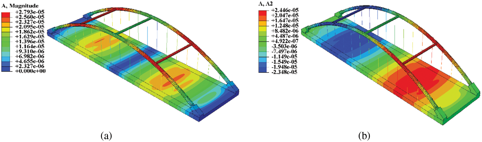
Figure 1: Spatial accelerations (a) x-direction, (b) y-direction

Fig. 2 shows examples of the joint’s nonlinear dynamic time history for strain and stress in the x axis, while Fig. 3 shows examples of the joint’s nonlinear dynamic time history for acceleration in the x and y axes. These structural responses are used for further analysis.

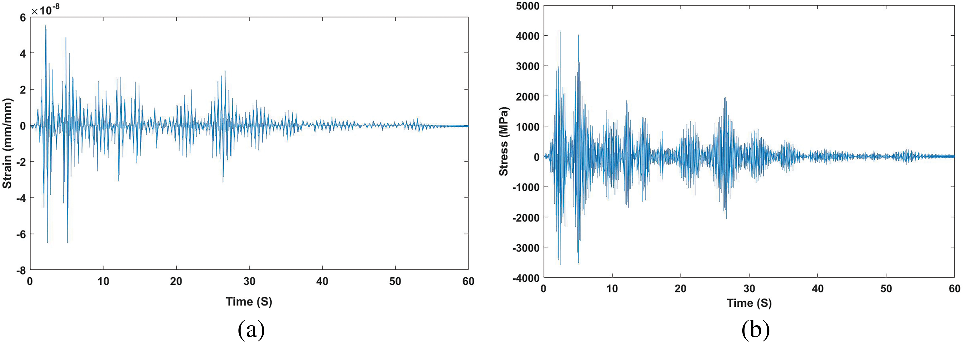
Figure 2: Examples of the joint’s nonlinear dynamic time history for (a) strain and (b) stress in the x axis

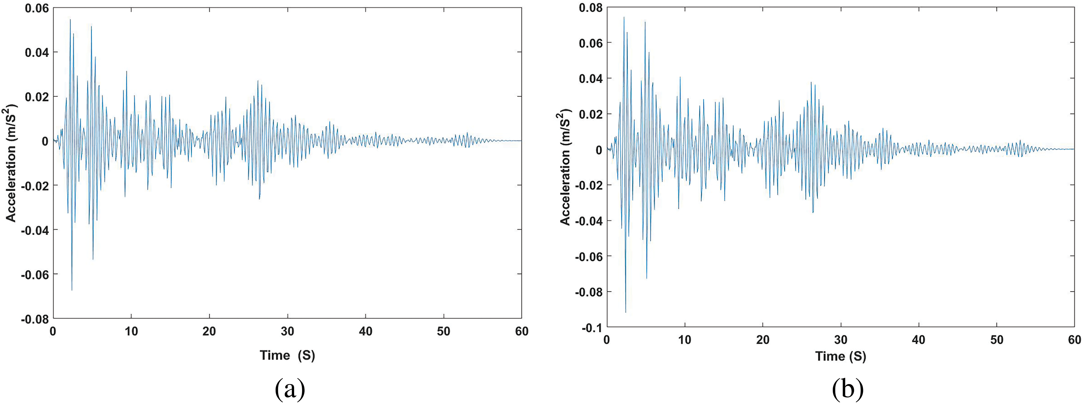
Figure 3: Examples of the joint’s nonlinear dynamic time history for acceleration in (a) x axis and (b) y axis

4.2 Time Frequency Analysis Based EMD Algorithm and Hilbert-Huang Transform

Empirical mode decomposition (EMD) is a data-adaptive multiresolution technique to decompose a signal into physically meaningful components [27]. It can be used to analyze non-linear and non-stationary signals by separating them into components at different resolutions and can be used to perform time-frequency analysis while remaining in the time domain. The components are in the same time scale as the original signal, which makes them easier to analyze. The EMD principle is to decompose adaptively a given signal into IMFs extracted from the signal by means of the sifting process. The name IMF is adapted because it represents the oscillation mode embedded in the data [28]. With this definition, the IMF in each cycle, defined by the zero crossings of, involves only one mode of oscillation, no complex riding waves are allowed. Thus, an IMF is not restricted to a narrow band signal, and it can be both amplitude and frequency modulated. The EMD picks out the highest frequency oscillation that remains in the signal. Thus, locally, each IMF contains lower frequency oscillations than the one extracted just before. Also, the EMD does not use any pre-determined filter, it is a fully data driven method. Since the EMD decomposition is based on the local characteristics time scale of the data, it is applicable to nonlinear and nonstationary processes. Having obtained the IMFs using the EMD method, one applies the Hilbert transform to each IMF component to obtain its amplitude and phase angle, which are used to estimate the natural frequencies and damping ratios of a civil structure [27]. However, in this study, the IF and IA of the separated of an amplitude modulation-frequency modulation (AM-FM) signal IMFs are calculated using the discrete energy separation algorithm (DESA). Fig. 4 analysis technique based on Empirical mode decomposition.

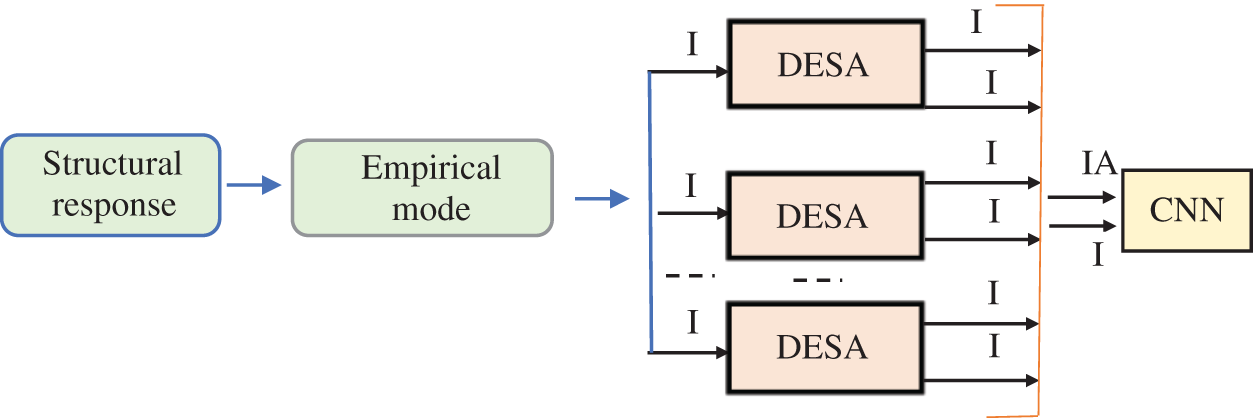
Figure 4: Analysis technique based on Empirical mode decomposition

EMD is used as a multiband filtering to separate the signal components in the time domain and hence reduce multicomponent demodulation to multicomponent one. DESA is used to track the IF and IA of a monocomponent AM-FM signal. The Teager energy operator captures the nonlinearity in the signal and is used to compute the time-frequency representation of the signal. Each of these steps is crucial in extracting meaningful insights from large and complex datasets. The sifting process helps analysts and researchers focus on the most pertinent information, thus enabling informed decision-making or further research.

4.3 Hilbert-Huang Transform

Apply the Hilbert transform to each IMF obtained from the EMD process. This results in a complex-valued signal for each IMF, forming the analytic signal. Having obtained the IMFs using the EMD method, one applies the Hilbert transform to each IMF component. With this definition ci(t) and H[ci(t)] form a complex conjugate pair, which defines an analytic signal zi(t) [28]:

zi(t)=ai(t)exp(jωi(t)) (1)

Amplitude and Phase: For each IMF, extract the amplitude ai(t) and phase θi(t) from the complex analytic signal:

ai(t)=ci(t)2+H[ci(t)]2 (2)

θi(t)=arctan(H[ci(t)]ci(t)) (3)

Instantaneous Frequency: Compute the instantaneous frequency ωi(t) as the derivative of the phase with respect to time. Therefore, the instantaneous frequency ωi(t) can be given by:

ωi(t)=dθi(t)dt (4)

Instantaneous Amplitude: The instantaneous amplitude a(t) is the magnitude of the complex analytic signal:

a(t)=∑i=1N⁡ai(t)2 (5)

Thus the original data can be expressed in the following form:

x(t)=Re∑i=1n⁡ai(t)exp(j∫ωi(t)dt) (6)

where the residue rn(t) has been left out. Re {.} denotes the real part of a complex quantity. Eq. (6) enables us to represent the amplitude and the instantaneous frequency, in a three-dimensional plot, in which the amplitude is the height in the time-frequency plane. This time-frequency distribution is designated as the Hilbert-Huang spectrum H(ω, t) :

H(ω, t)=Re∑i=1n⁡ai(t)exp(j∫ωi(t)dt) (7)

This process allows you to characterize the time-varying frequency and amplitude components present in the original acceleration data. It’s a powerful approach for analyzing non-stationary signals.

ω[n]=dφ[n]dn (8)

ζ[n]=1ω[n]A[n]A[n]′ (9)

The terms ωi(t) is instantaneous frequency, θi(t) is the phase with respect to time, a(t) is instantons amplitude, ai(t) is the magnitude of the complex analytic signal for the i-th component; φ[n] is phase used in the discrete form of instantaneous frequency; ζ[n] is the damping ratio in discrete form; A[n]  is magnitude in discrete form; A[n]′ is derivative of magnitude in discrete form.

4.4 Discussion and Results Analysis

Figs. 5 and 6 in the study show the Intrinsic Mode Functions (IMFs) derived from the vibration measurements. IMFs are obtained using the Empirical Mode Decomposition (EMD) method, which decomposes the vibration signals into a set of functions that represent the inherent oscillatory modes of the bridge. In Fig. 5, there are 9 plots, each representing an IMF component over time in seconds. The IMFs seem to be capturing different frequency components within the vibration signal, which is typical in EMD analysis. This figure is a baseline measurement, which suggests that this is the reference state of the structure under normal conditions or before any damage has occurred. Fig. 6 also shows 9 plots of IMFs over time in seconds. The appearance of the IMFs suggests more prominent fluctuations, especially in the last plot (IMF9), which could indicate changes in the structural conditions, such as the presence of damage or alterations in the dynamic properties of the structure. The amplitude of the fluctuations in the Fig. 6 seems larger, especially in the lower order IMFs (e.g., IMF9). This might be a sign of increased vibration levels, possibly due to damage or changes in the structural integrity. The patterns in the Fig. 5 are relatively uniform, whereas the Fig. 6 shows more variability. In structural health monitoring, changes in pattern or amplitude can signify changes in the physical state of the structure. The comparison suggests that there might be significant differences between the baseline and current conditions, indicating potential changes in the structural health of the bridge. However, to draw conclusive insights regarding the structural health, engineers would usually conduct further analyses involving more comprehensive data, potentially including other types of sensors and longer monitoring periods, to confirm any findings suggested by the IMF comparisons.

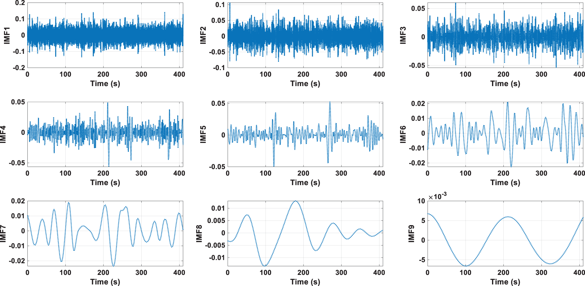
Figure 5: The IMFs component of vibration measurement of baseline of bridge condition

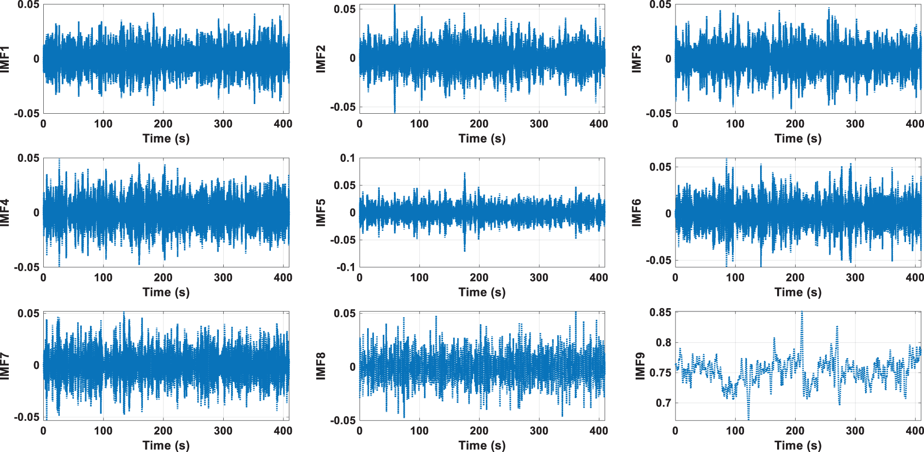
Figure 6: The IMFs component of vibration measurement of current bridge condition

Figs. 7 and 8 depict the instantaneous frequency content of Intrinsic Mode Functions (IMFs) derived from vibration data of a bridge, analyzed using Hilbert-Huang Transform (HHT). This type of analysis is crucial in structural health monitoring to identify changes in the structural characteristics of the bridge over time, which can be indicative of damage or deterioration. The Figure of baseline condition shows the frequencies are relatively stable over time, with only a few fluctuations. This stability suggests no significant structural changes or damages at the time of this measurement. The lower frequency content in some IMFs could be related to the fundamental structural frequencies of the bridge, and their stability is a sign of structural health [29]. The Figure of the current bridge condition compared to the baseline condition, shows that there are noticeable differences in the frequency content, with more fluctuations and some IMFs showing larger variations in frequency over time. The presence of these fluctuations and the change in frequency content could suggest potential structural changes or damage. For example, increases in frequency might indicate a loss of mass or stiffness in certain bridge components. The lower IMFs, which generally represent the dominant structural frequencies, seem to have more variability, which is particularly concerning from a structural health monitoring perspective. Also, the range of frequencies present in the current condition may have shifted or broadened compared to the baseline. A broader range could mean that new vibration modes are being excited due to changes in the structure. Also, the current condition plots show potential anomalies or sudden changes in frequency, especially at specific time intervals. These could correspond to events or defects affecting the bridge. In the context of structural health monitoring, comparing these figures allows engineers to detect changes in the structural behavior of the bridge over time. The variations in frequency content between the baseline and current conditions can be analyzed further to diagnose potential damages or to decide on maintenance actions. It’s important to consider that while some variability is expected due to environmental factors (like temperature and wind), significant deviations from the baseline can be a sign of structural issues that need to be addressed.

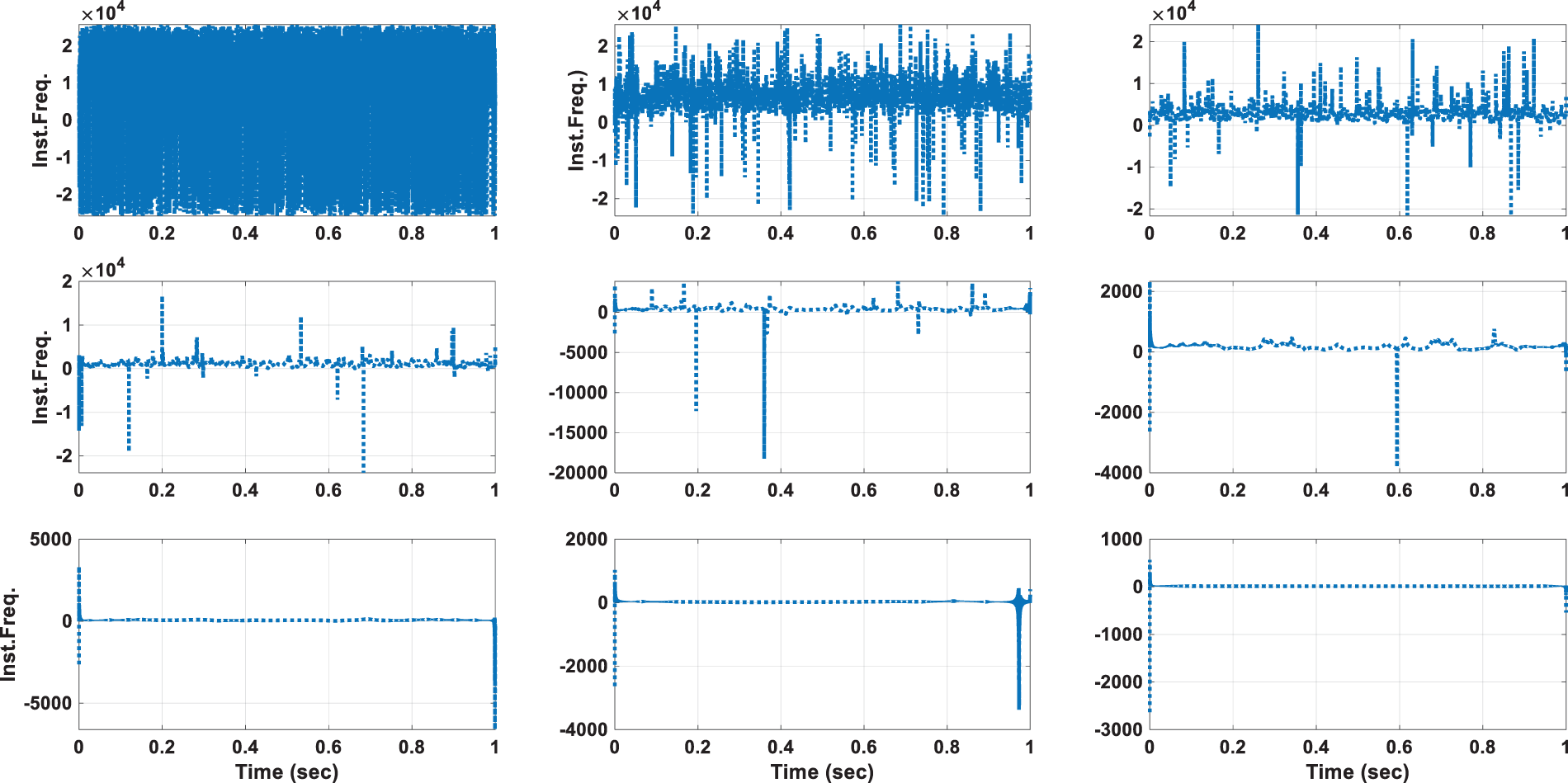
Figure 7: The instantaneous frequency of IMFs component of vibration measurement of baseline of bridge condition

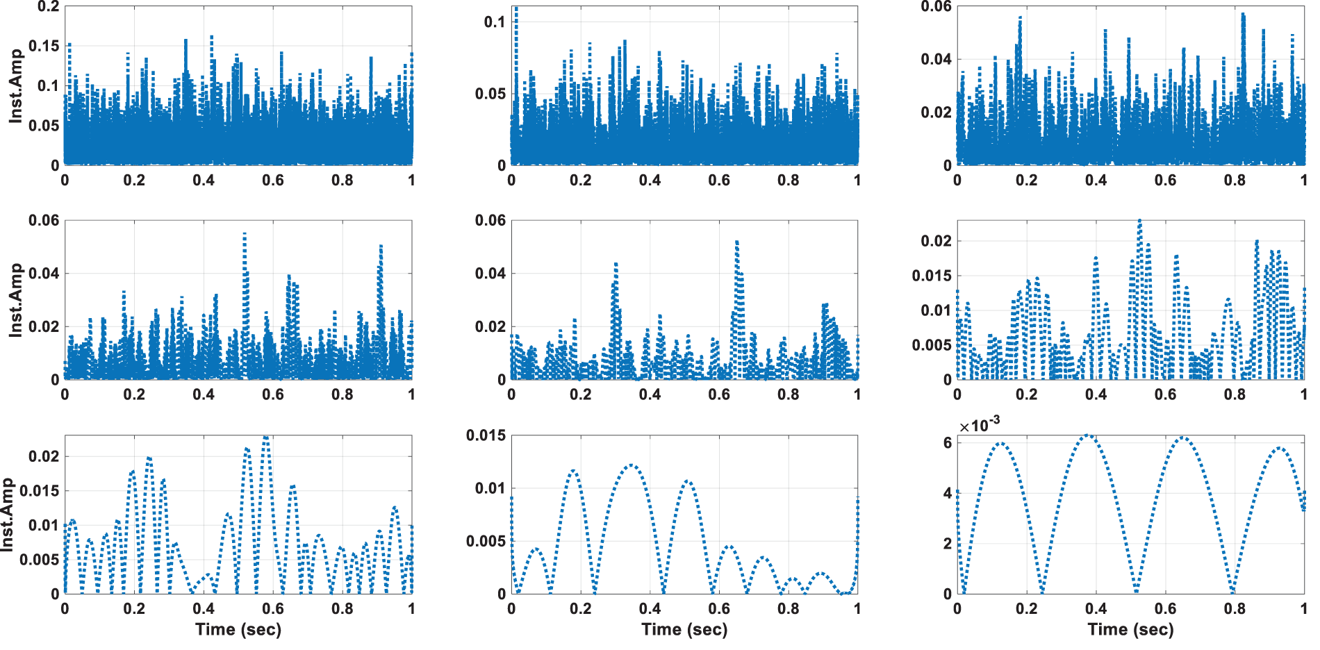
Figure 8: The instantaneous frequency of IMFs component of vibration measurement of current bridge condition

5  CNN Architecture

The machine learning (ML) in bridge health monitoring revolutionizes condition assessments by enabling accurate predictions and proactive maintenance strategies [30]. ML algorithms excel in anomaly detection, recognizing patterns, and predicting structural degradation [24]. This technology provides real-time monitoring capabilities, adaptability to dynamic conditions, and the ability to process data from diverse sensor networks. Regression analysis and ensemble learning enhance accuracy, while continuous learning ensures models remain relevant over time. ML-driven decision support facilitates prioritized maintenance, resource allocation, and long-term structural health planning. Overall, the ML in bridge health monitoring marks a transformative shift towards more adaptive, accurate, and predictive assessments, contributing to the resilience and safety of bridge infrastructure.

5.1 Convolutional Neural Network (CNN)

A CNN is a type of feed-forward neural network (FFNN), stands out as a cornerstone algorithm in the realm of deep learning. Based on the convolution kernel sliding operation characteristics, combined with the improved neural network algorithm, it can effectively understand and capture images. This makes it great for detecting things like cracks in images and it is currently the most commonly used image-based crack detection method [31,32]. A standard CNN architecture comprises essential components such as convolutional layers, pooling layers, activation functions, and fully connected layers, as depicted in Fig. 9.

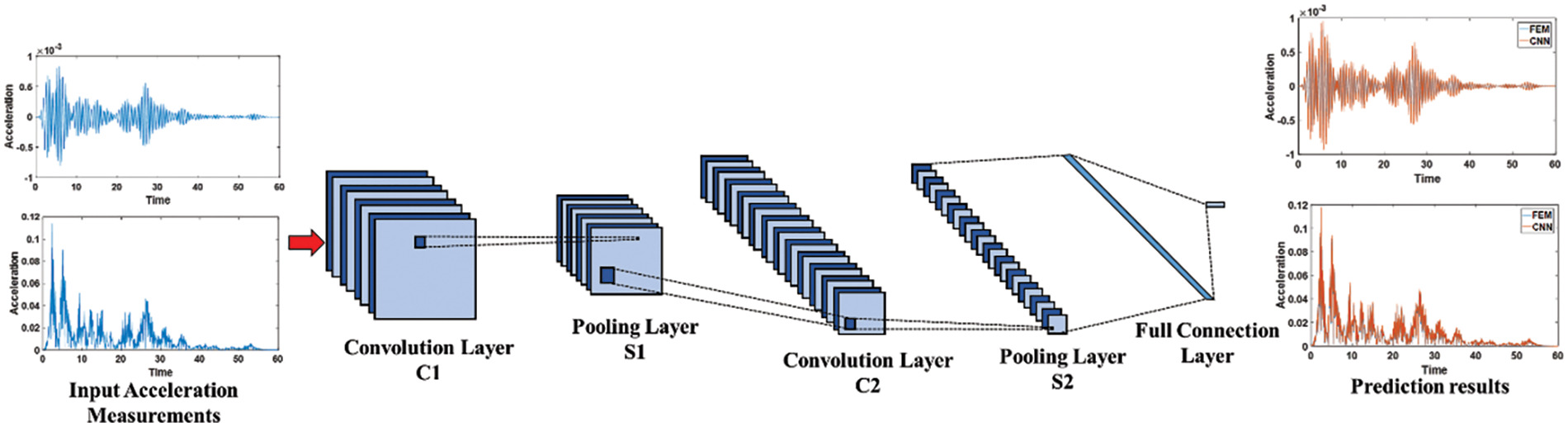
Figure 9: The architecture of a standard CNN

5.1.1 Convolution Layers

The convolutional layer serves as the heart of the CNN, playing a vital role in extracting features from input data. By applying a convolution operation with a pre-defined kernel, the layer can detect intricate details like image contours, and produce the corresponding feature map. Through this process, multiple input feature maps are combined, eventually leading to an output representation that covers the learned features. The output is expressed as the following:

xjl=f(∑i∈Mj⁡xil−1∗kijl+bjl) (10)

where Mj represents a set of input feature maps, and each output feature map is augmented with an additive bias b. The input feature maps undergo convolution with distinct kernels tailored for each output feature map.

5.1.2 Gradients in the Convolution Layers

The pooling layer works by either selecting the maximum or average value within a neighborhood, effectively downsampling the feature map or reducing its spatial size. Meanwhile, the activation function layer utilizes functions to process the input data. The widely used activation functions, such as the ReLU function and its variants, help introduce non-linearity into the network. In this process, each feature map j undergoes a similar computation as in the convolutional layer, alongside a corresponding map calculated in the pooling layer.

δjl=βjl+1(f′(ujl)∘up(δjl+1)) (11)

where up(⋅) denotes operation that up-sample the data, where each pixel in the input is replicated horizontally and vertically n times in the output if the subsampling layer reduces the data by a factor of n. The down-sampling layer l + 1 directly follows the convolution layer l for computation of calculate sensitivity, the units in layer l + 1 are connected to the relevant units in the current layer l, and these connections are assigned weights defined at layer l + 1. In this context, the weights at a down-sampling layer map are represented as β , and the previous result scaled by β is computed to achieve β . The gradients with respect to the bias bj and kernel weight kijl are expressed as follows:

∂E∂bj=∑u, v⁡(δjl)uv (12)

∂E∂kijl=∑u, v⁡(δjl)uv(pil−1)uv (13)

where (pil−1)uv is the patch in xil−1 multiplied by kijl through element wise process to compute the element at (u, v) in the output map xjl in the convolutional layer.

5.1.3 Sub-Sampling Layers

At a subsampling layer, down-sampled versions of the input maps are generated.

xjl=f(βjldown(xjl−1)+bjl) (14)

where down(⋅) represents a sub-sampling process.

5.1.4 Gradients in the Sub-Sampling Layers

Convolutional layers encase the subsampling layers both above and below. Parameters that can be learned, such as bias parameters β and b, require updating.

∂E∂bj=∑u, v⁡(δjl)uv (15)

∂E∂βj=∑u, v⁡(δjl∘djl)uv (16)

5.1.5 Learning Combinations of Feature Maps

Let αij denotes the weight that connects output map j and input map i . The output map j can be defined as:

xjl=f(∑i=1Nin⁡αij(xil−1∗kil)+bjl) (17)

Expose to the constraints:

∑i⁡αij=1 and 0≤αij≤1, (18)

The soft max derivative process can be defined as:

∂αk∂ci=δkiαi−αiαk (19)

While the error derivative regarding αi and ci is specified as:

∂E∂αi=∂E∂ul∂ul∂αi=∑u, v⁡(δl∘(xil−1∗kil))uv (20)

Here, the inputs u , δl denotes the sensitivity map concerning an output map. To compute the error gradients of the network with respect to the underlying weights ci , a chain rule is applied:

∂E∂ci=∑k∂E∂αk∂αk∂ci=αi(∂E∂αi−∑k∂E∂αkαk) (21)

5.1.6 Enforcing Sparse Combinations

The weights distribution αi is subjected to ωsparseness constraints for a given map by including a regularization penalty term Ω(α) into the final error function. The regularization penalty Ω(α) can be derivative as:

∂Ω∂αi=λsign(αi) (22)

∂Ω∂ci=∑k∂Ω∂αk∂αk∂ci=λ(|αi|−αi∑k⁡|αk|). (23)

The study provides examples to elucidate convolution and pooling processes, with illustrations in Figs. 10 and 11 showing the convolution process. Specifically, the study employs average pooling as demonstrated.

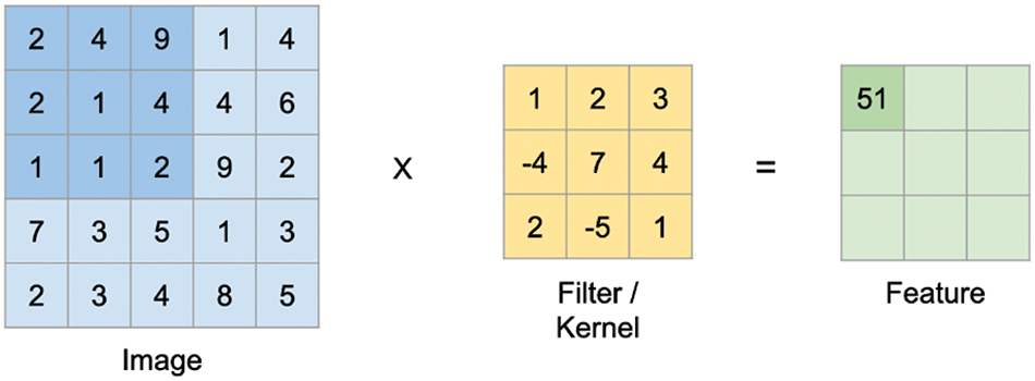
Figure 10: The input data is 7 × 7 × 3 dataset, where 7 × 7 represents width and height (pixels), and 3 represents B R G color channels

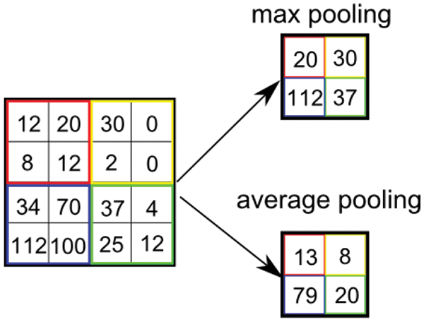
Figure 11: Max and average pooling operation in the CNN algorithm

In the fully connected layer, each neuron is linked to every neuron in the preceding layer. Activated neurons in the trained CNN model contribute to scoring the category of the predicted image. The selected loss function, typically cross-entropy loss, computes the training loss. Subsequently, weights are updated using the backpropagation (BP) algorithm and gradient descent. Stochastic gradient descent stands out as the most favored method for implementing gradient descent, due to its widespread adoption.

5.2 Training and Optimization

The damage scenarios used for training the CNN are derived from vibration measurements collected at various intervals, each interval representing a specific condition of the bridge. These datasets are systematically partitioned into training, testing, and validation sets to ensure comprehensive model development and evaluation. The training process for the CNN in bridge health monitoring adopts a comprehensive approach. It commences with transfer learning, utilizing pre-trained models for associated tasks, and then fine-tunes them on the task-specific bridge health dataset. Data augmentation techniques improve generalization, while optimization algorithms minimize the loss function, including regularization approaches to avoid overfitting. Ensemble training coordinates multiple CNN modules to collectively contribute to overall predictive capabilities. Cross-validation evaluates generalization performance, and nonstop monitoring and updating mechanisms adapt the models to evolving bridge health patterns. This holistic training process confirms a CNN group is optimized for adaptive, accurate, and robust structural health assessments. Strategies for handling challenges in bridge monitoring include resampling techniques to handle class imbalance, synthetic data generation for minority class representation, weighted loss functions to adjust for address prevalence, ensemble approaches for anomaly detection and noise reduction to recognize and treat outliers, hard data quality checks, considerate feature engineering, adaptive learning for continuous adaptation, regularization techniques to avoid overfitting, and expert consultation for nuanced problem-solving. These strategies collectively improve the model’s robustness, accuracy, and reliability in monitoring and evaluating the bridges health. This approach allows the CNN to effectively learn and predict the current condition of the bridge based on the vibration data.

Table 1 provides detailed settings for a convolution layer, where C1 denotes the first convolutional layer comprising six feature maps. Each feature map neuron has an 8×8 connection size to the input matrix, resulting in feature maps sized 148×148  matrices. There are a total of four filters, each with 8×8 unit parameter weights and a bias parameter, amounting to (8×8 + 1) × 4 = 260 tuned parameters. With one kernel between the input and the first convolutional layer C1 , the total connections amount to 260 × (148×148) = 5,695,040 . A sub-sampling layer S1 , having (1 + 1) × 2 = 4 tuned parameters and (4×4 + 1) × 2 × (64×64) = 139,264 connections, follows this, along with similar architectures for the subsequent layers, C2 and S2 , as depicted in Table 1. Essential parameters for CNN training are outlined in Table 2. Fig. 12 illustrates the training performance using supervised mode, while Algorithm 1 delineates the training and evaluation procedures conducted using MATLAB software.

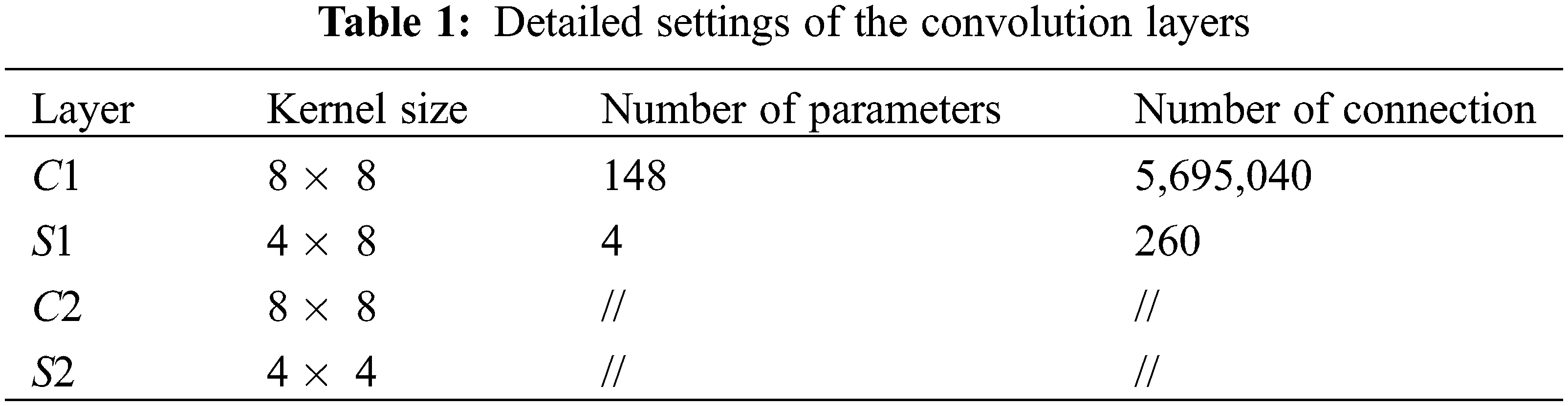
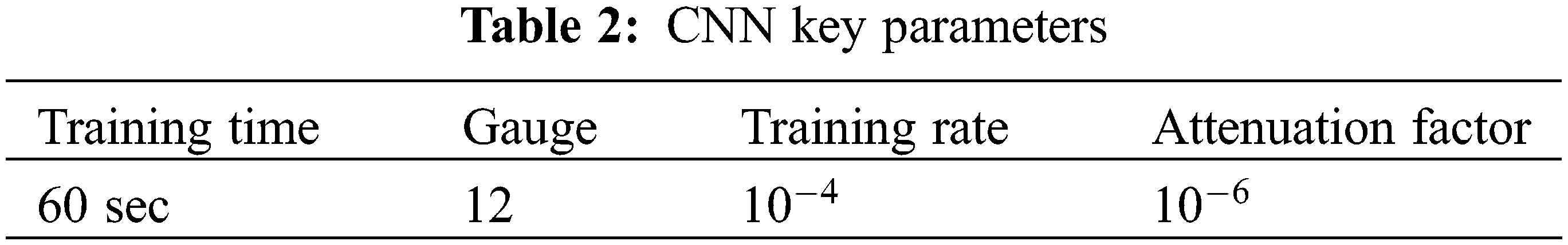
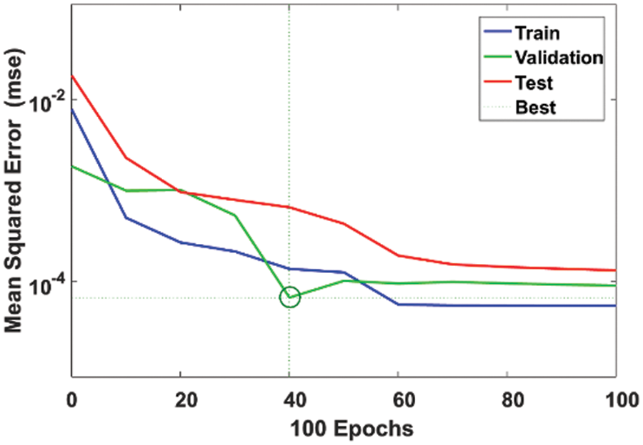
Figure 12: CNN training performance

Figs. 13 and 14 provide a comparison between CNN-predicted data and FEM results for the nonlinear dynamic time history of joint acceleration in the x and y axes, as well as stress and strain in the x axis. As depicted in the figures, the CNN demonstrates significantly improved prediction quality for this case study, showing its effectiveness in accurately modeling the structural behavior.

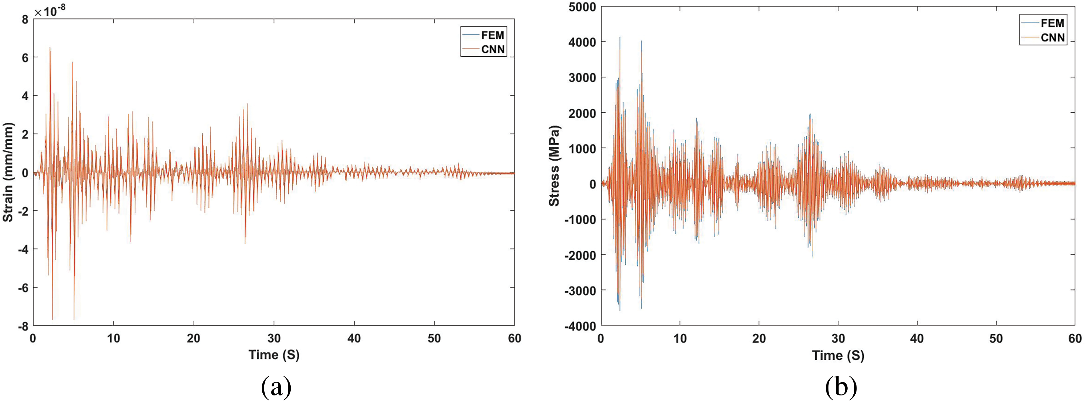
Figure 13: A comparison between CNN and FEM results of joint’s nonlinear dynamic time history for (a) strain and (b) stress in the x axis

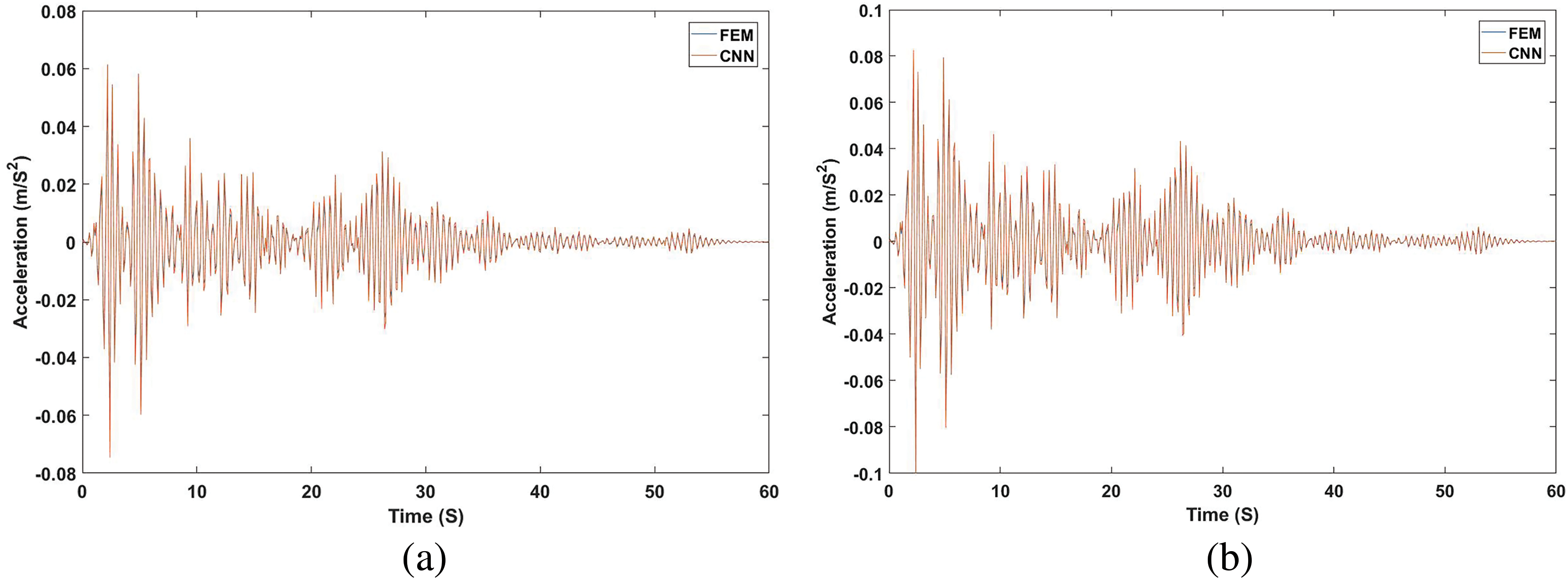
Figure 14: A comparison between CNN and FEM results of the joint’s nonlinear dynamic time history for acceleration in (a) x axis and (b) y axis

6  Conclusion

This study provides a comprehensive analysis of the vibrational characteristics of the bridge by comparing baseline and current conditions using Intrinsic Mode Functions (IMFs) and CNN. The comparison reveals significant changes in the vibrational patterns, indicating potential structural issues. Specifically, there is an increase in amplitude variability across several IMFs, particularly in IMF4 to IMF9. In the baseline condition (Fig. 5), IMF4, IMF5, and IMF6 have peak values of around 0.05, whereas, in the current condition (Fig. 6), these IMFs show an increase in amplitude variability, with peak values of around 0.1. Similarly, IMF7 and IMF8 in the baseline condition have peak values around 0.02, but in the current condition, they increase to approximately 0.05. IMF9 shows a substantial change from peak values of 0.002 in the baseline to around 0.08 in the current condition. These changes suggest that the bridge has experienced structural modifications that could indicate damage or deterioration, such as material fatigue, joint loosening, or other structural degradations. The quantitative differences in the IMFs’ amplitudes highlight the need for further inspection and possible maintenance to address these changes.

The effectiveness of the CNN model is demonstrated by a significant decrease in the mean squared error (MSE) from 10−2 to 10−4 over 100 epochs, as shown in Fig. 12. Figs. 13 and 14 compare CNN and Finite Element Method (FEM) results for strain, stress in the x axis, and acceleration, showing close alignment and validating the CNN’s accuracy in predicting the bridge’s structural response under dynamic loading conditions. This quantitative validation supports CNN’s utility in practical structural health monitoring applications, ensuring the bridge’s long-term safety and functionality.

The findings underscore the importance of continuous monitoring and predictive modeling to ensure the bridge’s safety and longevity. By analyzing the vibration data at various intervals, we can accurately predict the current condition of the bridge and implement timely interventions to maintain its structural integrity. The observed changes in vibrational characteristics, particularly the increased amplitudes in IMFs4 through 9, indicate potential structural issues that require immediate attention to prevent further degradation. This study contributes to the field of structural health monitoring by demonstrating the effective use of CNNs for predicting bridge conditions based on high-frequency vibration measurements. It highlights the value of using Intrinsic Mode Functions (IMFs) to analyze vibrational characteristics and sets a precedent for proactive maintenance strategies, ensuring the long-term durability and safety of critical infrastructure.

Acknowledgement: None.

Funding Statement: This research received no specific grant from any funding agency in the public, commercial, or not-for-profit sectors.

Author Contributions: Conceptualization, Wael A. Altabey, Ahmed Silik, and Nabeel S. D. Farhan; methodology, Wael A. Altabey, Ahmed Silik, and Nabeel S. D. Farhan; software, Mohammad Noori, and Wael A. Altabey; validation, Yadong Xu, Weixing Hong, Mohammad Noori, and Wael A. Altabey; formal analysis, Yadong Xu, Weixing Hong, Ahmed Silik, and Nabeel S. D. Farhan; investigation, Mohammad Noori, and Wael A. Altabey; resources, Yadong Xu, Weixing Hong, Ahmed Silik, and Nabeel S. D. Farhan; writing—original draft preparation, Wael A. Altabey, Ahmed Silik, and Nabeel S. D. Farhan; writing—review and editing, Wael A. Altabey, Ahmed Silik, and Nabeel S. D. Farhan; visualization, Yadong Xu, Weixing Hong, Ahmed Silik, and Nabeel S. D. Farhan; supervision, Mohammad Noori, and Wael A. Altabey. All authors reviewed the results and approved the final version of the manuscript.

Availability of Data and Materials: This research received no data availability statement.

Ethics Approval: Not applicable.

Conflicts of Interest: The authors declare that they have no conflicts of interest to report regarding the present study.

References

1. Karakostas C, Quaranta G, Chatzi E, Zülfikar AC, Çetindemir O, De Roeck G, et al. Seismic assessment of bridges through structural health monitoring: a state-of-the-art review. Bull Earthq Eng. 2023 Nov 30;22:1–49. doi:10.1007/s10518-023-01819-3. [Google Scholar] [PubMed] [CrossRef]

2. Alokita S, Rahul V, Jayakrishna K, Kar VR, Rajesh M, Thirumalini S, et al. Recent advances and trends in structural health monitoring. In: Structural health monitoring of biocomposites, fibre-reinforced composites and hybrid composites, 2019 Jan 1; Elsevier; p. 53–73. doi:10.1016/B978-0-08-102291-7.00004-6. [Google Scholar] [CrossRef]

3. Mustapha S, Yufeng H, Khoa N, Ulrike D. Structural health monitoring in civil structures based on the time series analysis. In: Proceedings of the 9th Austroads Bridge Conference (ABS2014), 2014 Oct; Sydney, Australia. [Google Scholar]

4. Silik A, Noori M, Ghiasi R, Wang T, Kuok SC, Farhan NS, et al. Dynamic wavelet neural network model for damage features extraction and patterns recognition. J Civ Struct Health Monit. 2023 Feb 18;13:1–21. doi:10.1007/s13349-023-00683-8. [Google Scholar] [CrossRef]

5. Ahmadian V, Aval SBB, Noori M, Wang T, Altabey WA. Comparative study of a newly proposed machine learning classification to detect damage occurrence in structures. Eng Appl Artif Intell. 2024;127:107226. doi:10.1016/j.engappai.2023.107226. [Google Scholar] [CrossRef]

6. Moallemi A, Burrello A, Brunelli D, Benini L. Model-based vs. data-driven approaches for anomaly detection in structural health monitoring: a case study. In: Proceedings of the 2021 IEEE International Instrumentation and Measurement Technology Conference (I2MTC), 2021 May 17–20; Glasgow, UK. [Google Scholar]

7. Azimi M, Eslamlou AD, Pekcan G. Data-driven structural health monitoring and damage detection through deep learning: state-of-the-art review. Sensors. 2020;20(10):2778. doi:10.3390/s20102778. [Google Scholar] [PubMed] [CrossRef]

8. Wang T, Noori M, Altabey WA, Wu Z, Ghiasi R, Kuok S, et al. From model-driven to data-driven: a review of hysteresis modeling in structural and mechanical systems. Mech Syst Signal Process. 2023;204:110785. doi:10.1016/j.ymssp.2023.110785. [Google Scholar] [CrossRef]

9. Ghahari F, Malekghaini N, Ebrahimian H, Taciroglu E. Bridge digital twinning using an output-only Bayesian model updating method and recorded seismic measurements. Sensors. 2022;22(3):1278. doi:10.3390/s22031278. [Google Scholar] [PubMed] [CrossRef]

10. Mendler A, Döhler M, Ventura CE. A reliability-based approach to determine the minimum detectable damage for statistical damage detection. Mech Syst Signal Process. 2021;154(107):561. doi:10.1016/j.ymssp.2020.107561. [Google Scholar] [CrossRef]

11. Limongelli MP, Chatzi E, Döhler M, Lombaert G, Reynders E. Towards extraction of vibration-based damage indicators. In: Proceedings of the 8th European Workshop on Structural Health Monitoring (EWSHM 2016), 2016 Jul 5–8; Bilbao, Spain. [Google Scholar]

12. Silik A, Noori M, Altabey WA, Ghiasi R, Wu Z. Comparative analysis of wavelet transform for time-frequency analysis and transient localization in structural health monitoring. Struct Durability Health Monit. 2021;15(1):1–22. doi:10.32604/sdhm.2021.012751. [Google Scholar] [CrossRef]

13. Lee YS, Vakakis AF, Mcfarland DM, Bergman LA. Crack detection and 1107 characterization techniques—an overview. Struct Control Health Monit. 2014;21:742–60. doi:10.1002/stc.1655. [Google Scholar] [CrossRef]

14. Salehi H, Burgueño R. Emerging artificial intelligence methods in structural engineering”. Eng Struct. 2018;171:170–89. doi:10.1016/j.engstruct.2018.05.084. [Google Scholar] [CrossRef]

15. Ying Y, GarrettJr JH, Oppenheim IJ, Soibelman L, Harley JB, Shi J, et al. Toward data-driven structural health monitoring: application of machine learning and signal processing to damage detection. J Comput Civ Eng. 2013;27(6):667–80. doi:10.1061/(ASCE)CP.1943-5487.0000258. [Google Scholar] [CrossRef]

16. Feng D, Feng MQ. Computer vision for SHM of civil infrastructure: from dynamic response measurement to damage detection—a review. Eng Struct. 2018;156:105–17. doi:10.1016/j.engstruct.2017.11.018. [Google Scholar] [CrossRef]

17. Gomes GF, Mendéz YAD, Da Silva Lopes Alexandrino P, Da Cunha SS, Ancelotti AC. The use of intelligent computational tools for damage detection and identification with an emphasis on composites—a review. Compos Struct. 2018;196:44–54. doi:10.1016/j.compstruct.2018.05.002. [Google Scholar] [CrossRef]

18. Spencer BF, Hoskere V, Narazaki Y. Advances in computer vision-based civil infrastructure inspection and monitoring. Engineering. 2019;5(2):199–222. doi:10.1016/j.eng.2018.11.030. [Google Scholar] [CrossRef]

19. Martucci D, Civera M, Surace C. Bridge monitoring: Application of the extreme function theory for damage detection on the I-40 case study. Eng Struct. 2023;279:115573. doi:10.1016/j.engstruct.2022.115573. [Google Scholar] [CrossRef]

20. Civera M, Mugnaini V, Zanotti FL. Machine learning-based automatic operational modal analysis: a structural health monitoring application to masonry arch bridges. Struct Control Health Monit. 2022;29(10):e3028. doi:10.1002/stc.3028. [Google Scholar] [CrossRef]

21. Ahmadi HR, Daneshjoo F, Khaji N. New damage indices and algorithm based on square time-frequency distribution for damage detection in concrete piers of railroad bridges. Struct Control Health Monit. 2015;22(1):91–106. doi:10.1002/stc.1662. [Google Scholar] [CrossRef]

22. Ahmadi HR, Momeni K, Jasemnejad Y. A new algorithm and damage index for detection damage in steel girders of bridge decks using time-frequency domain and matching methods. Structures. 2024;61:106035. doi:10.1016/j.istruc.2024.106035. [Google Scholar] [CrossRef]

23. Zha ZB, Bai Y, Yilmaz A, Sezen H. Deep convolutional neural networks for comprehensive structural health monitoring and damage detection. In: Proceedings of the 12th International Workshop on Structural Health Monitoring, 2019 Sep 10–12; Stanford, CA, USA. [Google Scholar]

24. Gao Y, Mosalam KM. Deep transfer learning for image-based structural damage recognition. Comput Aided Civ Infrastruct Eng. 2018;33(9):748–68. doi:10.1111/mice.12363. [Google Scholar] [CrossRef]

25. Mantawy IM, Mantawy MO. Convolutional neural network based structural health monitoring for rocking bridge system by encoding time-series into images. Struct Control Health Monit. 2022;29(3):e2897. doi:10.1002/stc.2897. [Google Scholar] [CrossRef]

26. Yoon J, Lee J, Kim G, Ryu S, Park J. Deep neural network-based structural health monitoring technique for real-time crack detection and localization using strain gauge sensors. Sci Rep. 2022;12(1):20204. doi:10.1038/s41598-022-24269-4. [Google Scholar] [PubMed] [CrossRef]

27. Perez-Ramirez CA, Amezquita-Sanchez JP, Adeli H, Valtierra-Rodriguez M, Romero-Troncoso RD, Dominguez-Gonzalez A, et al. Time-frequency techniques for modal parameters identification of civil structures from acquired dynamic signals. J Vibroeng. 2016;18(5):3164–85. doi:10.21595/jve.2016.17220. [Google Scholar] [CrossRef]

28. Liu T, Luo Z, Huang J, Yan S. A comparative study of four kinds of adaptive decomposition algorithms and their applications. Sensors. 2018;18(7):2120. doi:10.3390/s18072120. [Google Scholar] [PubMed] [CrossRef]

29. Yao Y, Tung STE, Glisic B. Crack detection and characterization techniques—an overview. Struct Control Health Monit. 2014;21(12):1387–413. doi:10.1002/stc.1655. [Google Scholar] [CrossRef]

30. Moghadam KY, Noori M, Silik A, Altabey WA. Damage detection in structures by using imbalanced classification algorithms. Mathematics. 2024;12(3):432. doi:10.3390/math12030432. [Google Scholar] [CrossRef]

31. Lin CF, Zhu JD. Hilbert-Huang transformation-based time-frequency analysis methods in biomedical signal applications. Proc Insti Mech Eng, Part H: J Eng Med. 2012;226(3):208–16. doi:10.1177/0954411911434246. [Google Scholar] [PubMed] [CrossRef]

32. Zhu X, Cao M, Ostachowicz W, Xu W. Damage identification in bridges by processing dynamic responses to moving loads: features and evaluation. Sensors. 2019;19(3):463. doi:10.3390/s19030463. [Google Scholar] [PubMed] [CrossRef]