
 Submit a Paper
 Propose a Special lssue
 Open Access
ARTICLE

Structural Health Monitoring by Accelerometric Data of a Continuously Monitored Structure with Induced Damages
Department of Innovation Engineering, University of Salento, Lecce, 73100, Italy
* Corresponding Author: Nicola Ivan Giannoccaro. Email:
Structural Durability & Health Monitoring 2024, 18(6), 739-762. https://doi.org/10.32604/sdhm.2024.052663
Received 10 April 2024; Accepted 22 May 2024; Issue published 20 September 2024
 View Full Text
 Download PDF
Abstract
The possibility of determining the integrity of a real structure subjected to non-invasive and non-destructive monitoring, such as that carried out by a series of accelerometers placed on the structure, is certainly a goal of extreme and current interest. In the present work, the results obtained from the processing of experimental data of a real structure are shown. The analyzed structure is a lattice structure approximately 9 m high, monitored with 18 uniaxial accelerometers positioned in pairs on 9 different levels. The data used refer to continuous monitoring that lasted for a total of 1 year, during which minor damage was caused to the structure by alternatively removing some bracings and repositioning them in the structure. Two methodologies detecting damage based on decomposition techniques of the acquired data were used and tested, as well as a methodology combining the two techniques. The results obtained are extremely interesting, as all the minor damage caused to the structure was identified by the processing methods used, based solely on the monitored data and without any knowledge of the real structure being analyzed. The results use 15 acquisitions in environmental conditions lasting 10 min each, a reasonable amount of time to get immediate feedback on possible damage to the structure.Keywords
Nomenclature
| OMA | Operational Modal Analysis |
| SHM | Structural Health Monitoring |
| SSI | Stochastic Subspace Identification |
Throughout history, there has been a constant pursuit of enhancing safety measures. As structures age and deteriorate, it becomes increasingly crucial to detect, assess, and mitigate potential risks, degradation, or collapse (e.g., [1]). This importance is further magnified by the growing frequency of catastrophic events to which structures are exposed.
Structural Health Monitoring (SHM) is recognized as the practice of implementing suitable strategies designed to detect damage in aerospace, civil, and mechanical engineering infrastructure. This involves continuously monitoring a structure or mechanical system over time through regularly spaced measurements. SHM plays a pivotal role in damage detection due to its significant implications for life safety, helping prevent potential disasters. Moreover, continuous monitoring and dynamic characteristics analysis of structures offer a solution to the limitations of visual inspection methods and are vital for ensuring long-term safety. Although various techniques have been developed over the years to identify critical situations, such as those based on image processing which represent some of the most recent advancements [2], vibration-based analysis remains one of the most intriguing methods available.
In the case of vibration-based SHM, it entails extracting damage-sensitive features (quantifiable parameters dependent on changes in dynamic responses such as shifting natural frequencies, mode shapes, strain levels, damping properties, and altering energy dissipation) from the acquired measurements (e.g., [3,4]). Subsequently, these features are statistically analyzed to evaluate the current state of the system’s health. For long-term SHM, the previous output is periodically updated with the latest information on the structure’s condition to determine whether it can continue to fulfill its intended function or not [3].
The Operational Modal Analysis (OMA) addresses the challenge of identifying the modal parameters of structures; a task that can be arduous, expensive, or restricted with traditional Experimental Modal Analysis (EMA), especially for large structures. It concentrates on determining modal parameters for systems subjected to one or more excitation sources occurring during normal system operation under environmental forces that cannot be directly measured [5]. Consequently, modal analysis, particularly OMA, has been extensively utilized in evaluating structural integrity by tracking changes in modal parameters over time for damage detection of wind turbines [6–8] or of bridges [9–12].
The main advantage of OMA for SHM lies in its ability to detect the structure integrity in its operative conditions in situ and non-destructive ways. Modal parameters can be determined using various algorithms; however, the extent of their changes varies based on factors such as the location, severity, and nature of the damage, as well as the sensitivity of the instrumentation employed for data collection; furthermore, usually, it’s necessary to improve data quality using filtering techniques [5].
With specific regard to OMA approach the present authors noticed a new commercial software from ARTeMIS [13] which has been developed to assist in identifying the presence of damages; in particular, such software [13] is designed in order to tackle the first level of identification in the Rytter’s classification (existence of damage) [14]. The ARTeMIS Modal software has already been widely endorsed for use in identifying the modal parameters of the specific system under examination [15–19]. However, it can also ensure the identification of potentially dangerous situations on the monitored structure, starting only from accelerometers records, without the necessity to evaluate modal parameters, and in a non-invasive manner [20–22]. Some methods that use this type of data, but not the software tool, are already present in the literature [23–27].
This work aims to analyze a new dataset continuously acquired over a year on a real-world structure subjected to ambient conditions to test the software SHM tool. The acquisition of this dataset has been carried out and made available from the research group of the Leibniz Universität Hannover in Germany [28]. As known by the scientific literature, the database has been used by the Hannover team to analyze the repeatability of the structure frequencies with respect to the different environmental conditions and to apply preliminary evaluation about the damage detection analysis [29–33]. The main novelty of the present work is the testing of two different methods (classic and robust, as explained in the next section) to detect damages through the acquired experimental data both when the structure is intact and when it is damaged. The SHM methodologies applied are not sensitive to natural changes in the dynamic behavior of the structure due to fluctuations in ambient conditions and show excellent results in determining the damage condition for all the cases considered.
In the subsequent sections, the work is organized as follows: in Section 2 the damage detection algorithm implemented in the software tool will be described, with particular attention to how it works in terms of theoretical background; then, in Section 3, attention will shift towards the specific system under examination, providing an overview of its characteristics and data acquisition features; finally, in Section 4 the results obtained from the analysis will be presented and discussed, and in Section 5 conclusions are drawn.
2 Tool and the Theoretical Background of System Modeling
The software application, ARTeMIS Modal [13], is herein used within the frame of Operational Modal Analysis (OMA) techniques.
To monitor the structural integrity of the truss tower, which will be presented in the next paragraph, the Structural Health Monitoring (SHM) tool offers various methods to detect potential damage by analyzing recorded measurement files and results obtained during periodic monitoring.
From a theoretical standpoint, the SHM tool in ARTeMIS software utilizes Stochastic Subspace Identification (SSI) to construct a reference state model, serving as the basis for evaluating the dynamics and structural condition of the system in question.
The subsequent section will provide a brief description of the SSI method, along with an explanation of how the SHM tool operates to identify the presence of potential damage.
2.1 Stochastic Subspace Identification Method
The differential equation in Eq. (1) is assumed to describe the vibration behavior of the structure under unknown ambient excitation:
where t denotes continuous time; M, C2, K
Eq. (1) effectively describes the vibration behavior of the structure, but it has some limitations for the analysis discussed in this paper. Firstly, it is formulated in continuous time, whereas measurements are mostly sampled at discrete-time intervals; then, noise modeling is essential, in fact, alongside the primary excitation force f(t) there could be additional unknown sources of excitation, so in cases where only output data is available, it is customary to substitute detailed knowledge of the excitation with the assumption that the system is stimulated by white noise [34]. Therefore, to address these issues, the equation of dynamic equilibrium, Eq. (1), will be transformed into a discrete-time stochastic state-space model.
The SSI allows the description of the system with a discrete state space model [34,35], starting with the introduction of the following definition:
where Ac
So, Eq. (1) can be transformed in the following state Eq. (3):
In practice, not all the DOFs are monitored, so assuming that the measurements are evaluated at only r sensor locations, and that these sensors can be accelerometers, velocity, or displacement transducers, the observation equation is:
with y(t)
Defining:
the Eq. (3) becomes:
where C
At this point, Eqs. (3) and (6) constitute a continuous-time deterministic state-space model.
Measurements are obtainable at discrete time instant kΔt, where Δt is the sample time; so, the mentioned equation becomes as follows in Eq. (7), after sampling, and including the stochastic components (noise):
with
where E is the expected value operator and
Now, the inputs remain unmeasurable in the case of ambient vibration, so it is not considered in the model (uk = 0), but the input is implicitly modeled by the noise terms with the previous assumption. In this way, the final stochastic discrete state space model to be considered is the following one:
It is assumed that the stochastic system is stationary, so the following equations must be considered:
where in Eq. (10),
After defining the previous set of equations in Eq. (9) that describe our system, the main objective is to construct the Hankel matrix. This matrix is crucial as it enables the derivation of matrices A and C, which are necessary for determining the eigenvalues and eigenvectors, and consequently the extraction of the modal parameters of the structure. As such, it is the core of the damage detection residuals methodology (explained in Section 2.2).
The SSI provides two methods to determine the Hankel matrix H and consequently the system matrices: a covariance-driven method and a data-driven one. The considered methodology [13] uses the second one, and it allows the definition of a matrix only by using the output measured data [33] as expressed in Eq. (11):
where i is a user-defined index of data shift, from which the number of block rows of the matrix depends, and each of them has m rows composed of the data corresponding to each DOF; a larger i leads to better estimates. It’s possible to use a smaller matrix, by considering only
As illustrated in Eq. (11), the Hankel matrix can be decomposed into two constituent matrices:
with the subscripts + and − refer to the size of the matrices; in particular, a matrix with subscript “+” has m(i+1) block rows, while a matrix with the subscript “−” has m(i-1) block rows. As the computation of Eq. (12) usually is a large matrix the calculation is in practice based on QR decomposition of the data matrices, see reference [35] for details.
The Hankel matrix is built in such a way that it enjoys the factorization property [36], hence as the product of the observability matrix and a sequence of state vectors.
The observability matrix Oi has the following formulation:
From Eq. (13), the system matrices A and C can be obtained, and so the modal parameters of the system too [18,35], by performing an eigenvalues decomposition; however, details on this procedure are outside the scope of this study because the modal parameters are not evaluated in the proposed damage detection methodologies.
So, once the Hankel matrix is obtained, it is necessary to perform a Singular Value Decomposition (SVD), to find the observability matrix and the other entities necessary to conduct the damage detection.
The SVD is performed according to Eq. (14) [20,34], with truncation at the desired model order n; which selection is left to the discretion of the user and may also depend on the specific problem [37]. However, the order n of the model must be at least twice as high as the number of modes (or poles) expected in the considered frequency band. This is because the modes appear in conjugated complex pairs, with each pair corresponding to a calculated mode. Therefore, given that the matrix is of order n (the order of the model), it is concluded that, at most, n/2 modes can be identified [18].
where U1 and V1 are orthonormal matrices that correspond to a collection of n left and right singular vectors related to n singular values S1 contained in a diagonal matrix and are called, respectively, the image and the co-image of a matrix. The matrices U0 and V0 are called the left and right null spaces of a matrix, respectively. They contain the left and right singular vectors that correspond to the singular values in S0 which approximate zero. The next subsection will discuss their use in the damage detection methodology.
The observability matrix
2.2 Damage Detection Residuals Methodology
Starting from the Hankel matrix and its SVD, it is possible to perform damage detection on the analyzed structure by defining a new parameter: a residual vector. This residual vector enables the detection of potential damages without the need to estimate modal parameters.
Let ζ represent a damage detection residual derived from damage-sensitive features extracted from measurement data in both the reference and the currently tested states, with ∑ζ denoting its asymptotic covariance matrix. Comparing measurements between the healthy and tested states involves expressing the residual as following a Gaussian distribution. If the features of the currently tested system statistically align with the baseline features, the mean value of the distribution is zero; otherwise, it differs from zero [20].
The definition of the residual depends on the chosen damage detection method. There are two ways to define the residual: the classic method and the robust one.
2.2.1 Classic Subspace-Based Residual
In the non-parametric version of the damage detection test (i.e., without the use of modal parameters), assuming a constant covariance excitation, the residual vector is defined as follows [38]:
where N is the number of samples acquired,
Once the residual reference vector is known, this must be calculated for every state to be tested. Each new residual vector is obtained by iteratively replacing in Eq. (16) the null space value S of the reference state with the one of the tested states and multiplying it always by the estimated Hankel matrix of the reference state.
When the test data statistically corresponds to the baseline data, the mean value of the residual in Eq. (16) is zero when the currently tested dataset is classified healthy, and it is different from zero when the currently tested data is collected from a damaged structure; to establish if the residual is significantly different from zero or not, a non-parametric test is conducted as in Eq. (17).
where
2.2.2 Robust Subspace-Based Residual
The second method that can be used to find the residual vector for each tested state is known to be more robust to the change of ambient excitation due to, for example, variations in temperature or wind conditions.
In this case, the residual is found as in Eq. (16) but using the estimate of the left singular vector
Then, also in this case, the
The huge dataset provided by the University of Leibniz University Hannover in Germany has been considered [28] to analyze the software’s performance. To obtain a structure exposed to natural sources of excitation, which exhibits damages of various intensities and at multiple locations throughout its lifetime, while also enabling long-term measurements, the Hannover research group has developed and installed the Leibniz University Test Structure for Monitoring (LUMO). This is a lattice mast structure standing at around 9 m tall, featuring 18 reversible damages spread across six levels; positioned outdoors, the system is equipped with accelerometers, strain gauges, and a temperature sensor, ensuring continuous monitoring (Fig. 1). An adjacent meteorological measurement mast, located roughly 20 m away, offers a comprehensive assessment of environmental conditions. All collected data, from August 2020 to July 2021, alongside a reference finite element model, are available online through an open-access repository.
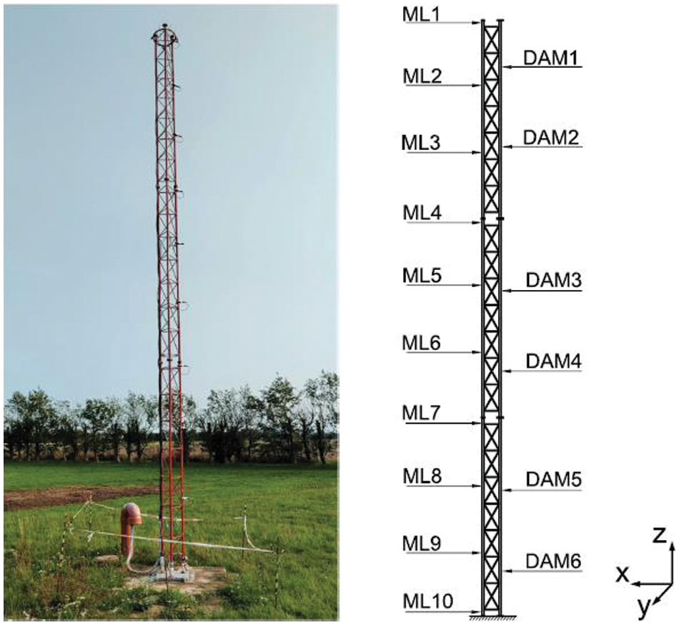
Figure 1: Test structure (left) and scheme of the measurement levels and damaged locations on the structure (right) (image is from [28])
As described in [28], and shown in Fig. 1, the steel lattice mast consists of three identical segments, each measuring 3 m in length, resulting in a total height of 9 m. Its overall weight, excluding sensors, is approximately 90 kg. Each segment features three tubular legs arranged to form a cross-section resembling an isosceles triangle (Fig. 2). Additionally, they consist of seven bracing levels, along with short connecting sections at the ends. The sections terminate in an elliptical flange, facilitating the assembly of segments in any order using standard M10 steel bolts. It is assumed that the structural steel used in the structure is characterized by Young’s modulus equal to 2.1 GPa and Poisson’s ratio equal to 0.3.
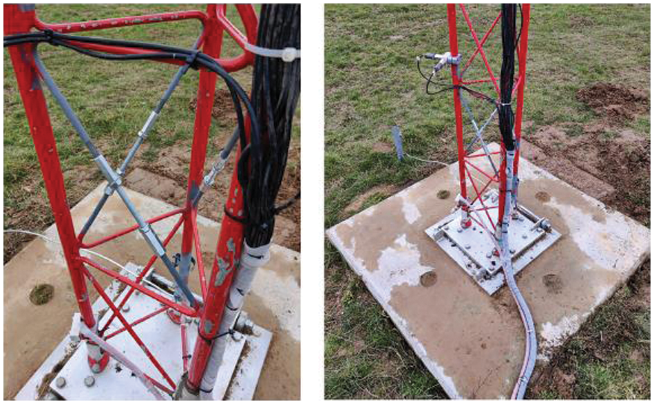
Figure 2: Photograph of the first bay and damage mechanism (left), and photograph of the placement of the first couple of accelerometers (right) (image is from [28])
The primary characteristic of the test structure revolves around localized reversible damages, which are evident through changes in stiffness and mass. To achieve this, reversible damage mechanisms are positioned across six levels of the structure, as illustrated in Fig. 1 (named DAM1, DAM2, DAM3, DAM4, DAM5, and DAM6), allowing for the detachment of individual bracings. The damage’s features comprise two screw sockets, one with a left-hand and the other with a right-hand thread, along with a connecting piece (threaded M10 rod). An exemplary image illustrating the damage mechanisms at damage level 6 is provided in Fig. 2. Activation of the damage mechanisms involves loosening the screw sockets and potentially removing the connecting pieces, resulting in the complete separation of the corresponding bracings.
The structure is equipped with 18 uniaxial accelerometers, three strain sensors (whose information will not be used in this work), and one temperature sensor, distributed across ten horizontal measurement levels (MLi, i = 1,…,10), as reported in Table 1 and described in Fig. 1. The piezoelectric accelerometers are installed in pairs utilizing 90° mounting brackets to measure orthogonal deflection directions, thus capturing spatial motion in the horizontal plane. No acceleration sensors are positioned in the vertical direction (z-axis) due to their limited significance for beam-like structures. The positioning and orientation of the accelerometers are schematically illustrated in Fig. 3.
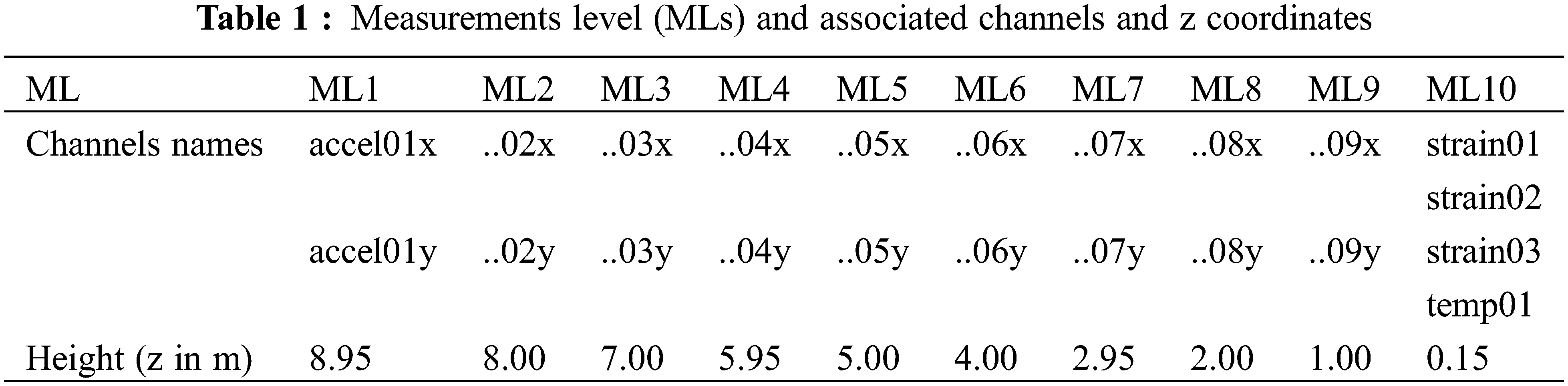
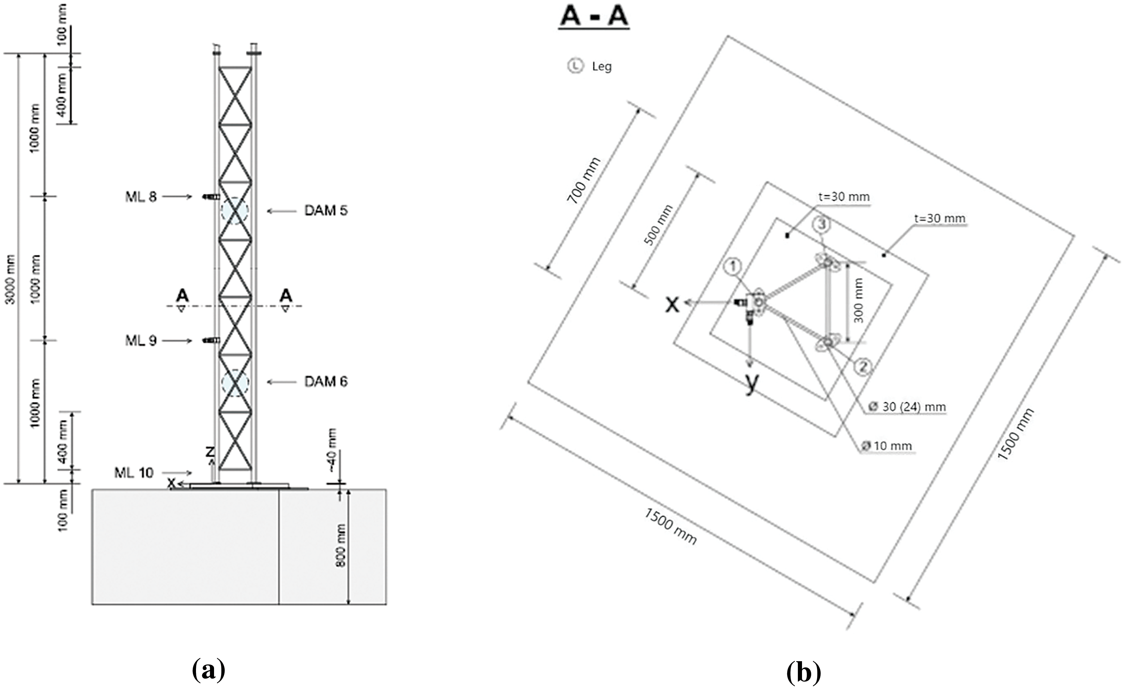
Figure 3: Front view of lower segment (a) and cross-section with measurement directions of accelerometers (b) (image is from [28])
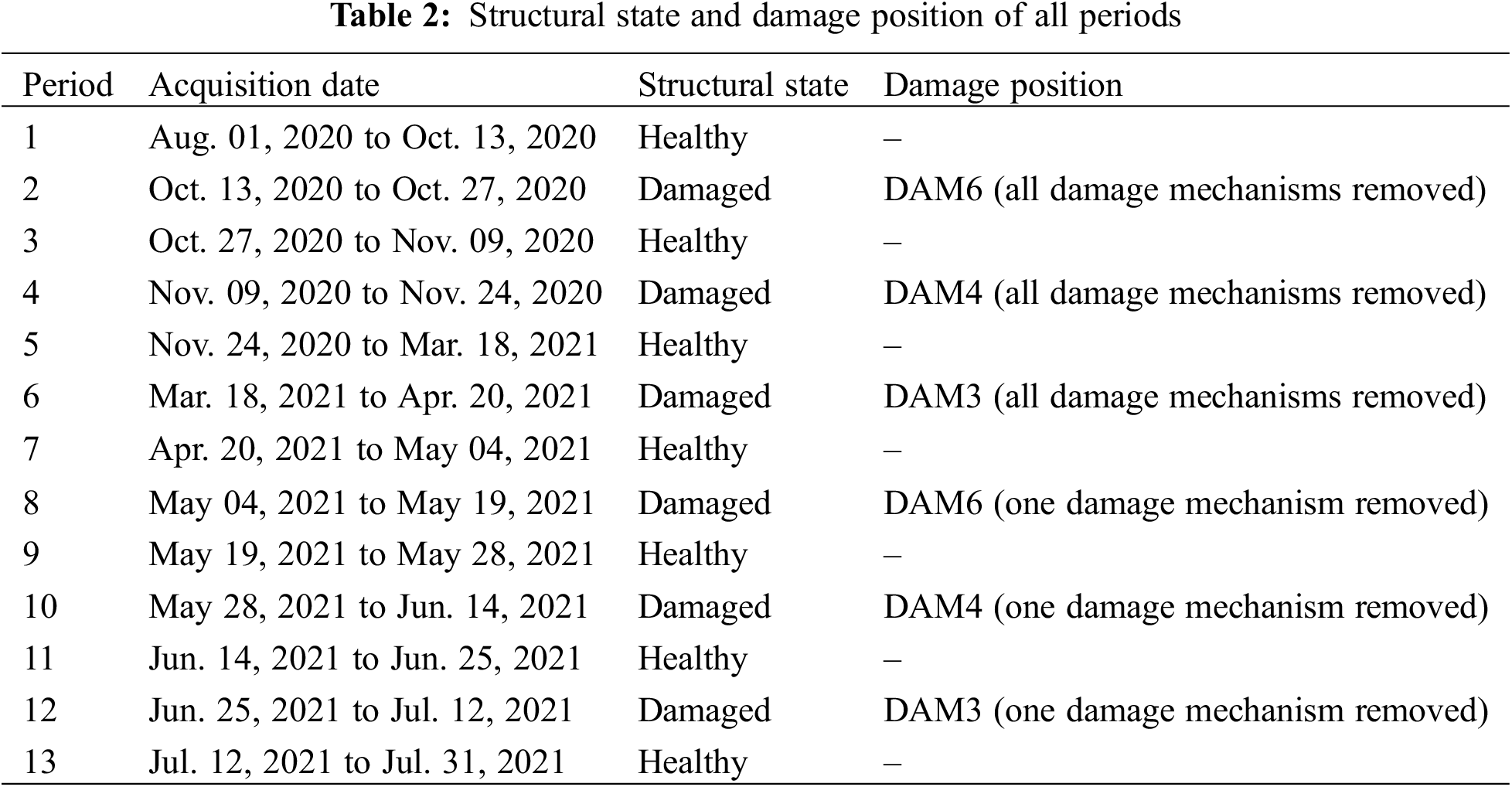
The database includes data obtained from measurements conducted on the undamaged structure, along with six instances of damage occurring at two varying levels of severity across three distinct locations, as outlined in Table 2.
The analyzed structure can be represented in ARTeMIS Modal as shown in Fig. 4. The observed database is constructed utilizing about 990,600 samples for each accelerometer, with a sampling frequency of 1651.6 Hz: data has been recorded every 10 min, each day from August 2020 to July 2021. To streamline the calculation, the software automatically reduces the samples considered, as far as the reference accelerometers. Users have the option to manually select reference accelerometers; nevertheless, tests conducted with various reference accelerometers yielded results that were not significantly different, therefore, the ones chosen by the software were deemed suitable (i.e., the 5 reference accelerometers are the purple ones in Fig. 4).
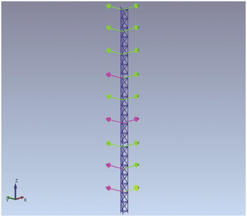
Figure 4: Representation of the analyzed structure in ARTeMIS Modal software
For each investigation, the resulting graphs are shown as follows: in Figs. 5 and 6 the frequencies graph of the first kind of damage is reported, Figs. 7 and 8 show the results related to the damage that occurred at level 6 with all mechanisms removed (DAM6), Figs. 9 and 10 show the results related to the damage occurred at level 4 with all mechanisms removed (DAM4), Figs. 11 and 12 show the results related to the damage occurred at level 3 with all mechanisms removed (DAM3); starting from Fig. 13 all the results related to damage obtained removing one strut at the time are reported, so Figs. 13 and 14 show this result for single damage occurred at level 6, Figs. 15 and 16 for single damage at level 4, and Figs. 17 and 18 for single damage occurred at level 3; finally, Fig. 19 shows the results obtained over all periods. In Figs. 7–18; a total of 30 sessions have been analyzed. The first 15 sessions in the graphs correspond to the healthy state, while the second 15 sessions pertain to the damaged state. The entire database comprises approximately 52,560 recordings, resulting from records conducted every 10 min, amounting to 144 recordings per day over a year. Hence, the analyzed sessions have been randomly selected for each period of the entire database to represent both healthy and damaged conditions.
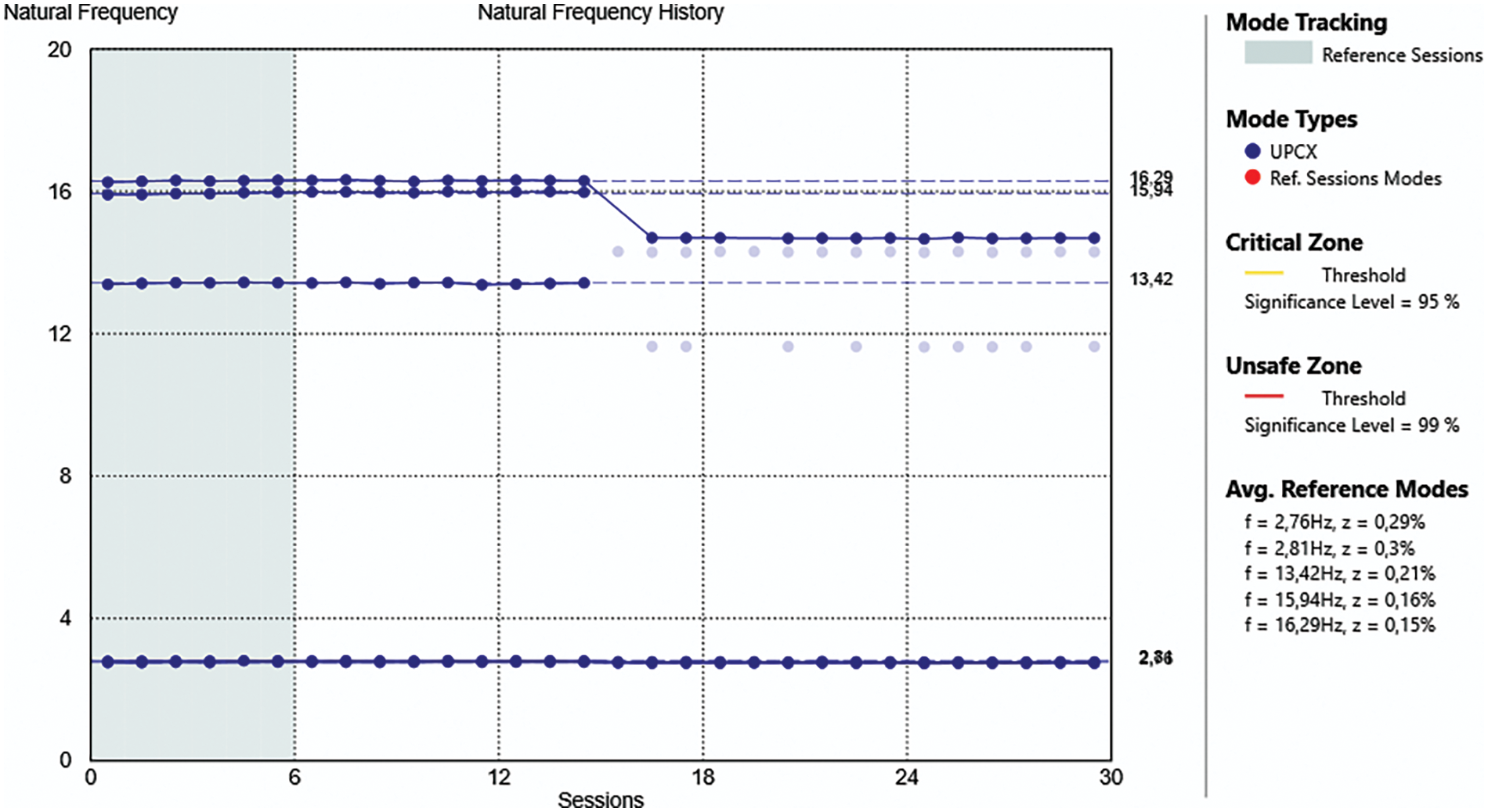
Figure 5: Frequency shift when damage at structure’s level 6 has occurred
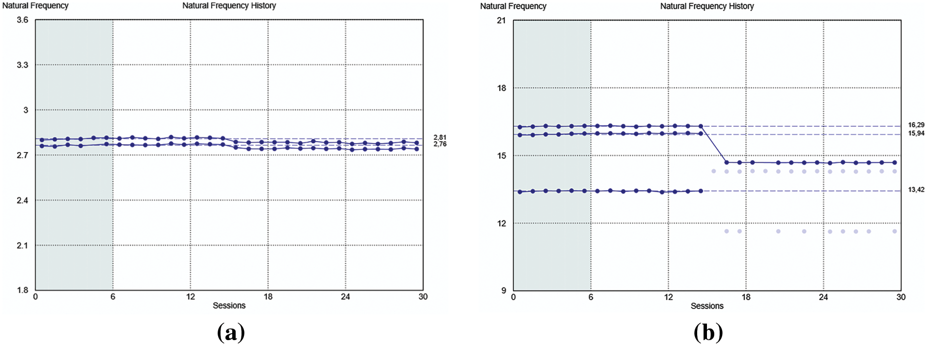
Figure 6: Zoom in on the first two frequencies (a) and on the subsequent three (b)
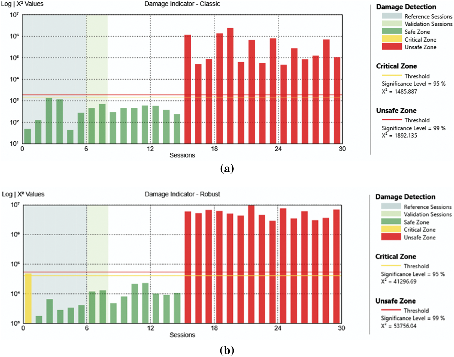
Figure 7: Analysis result of the case with damage at level 6 all mechanisms removed with classic algorithm (a) and robust algorithm (b)
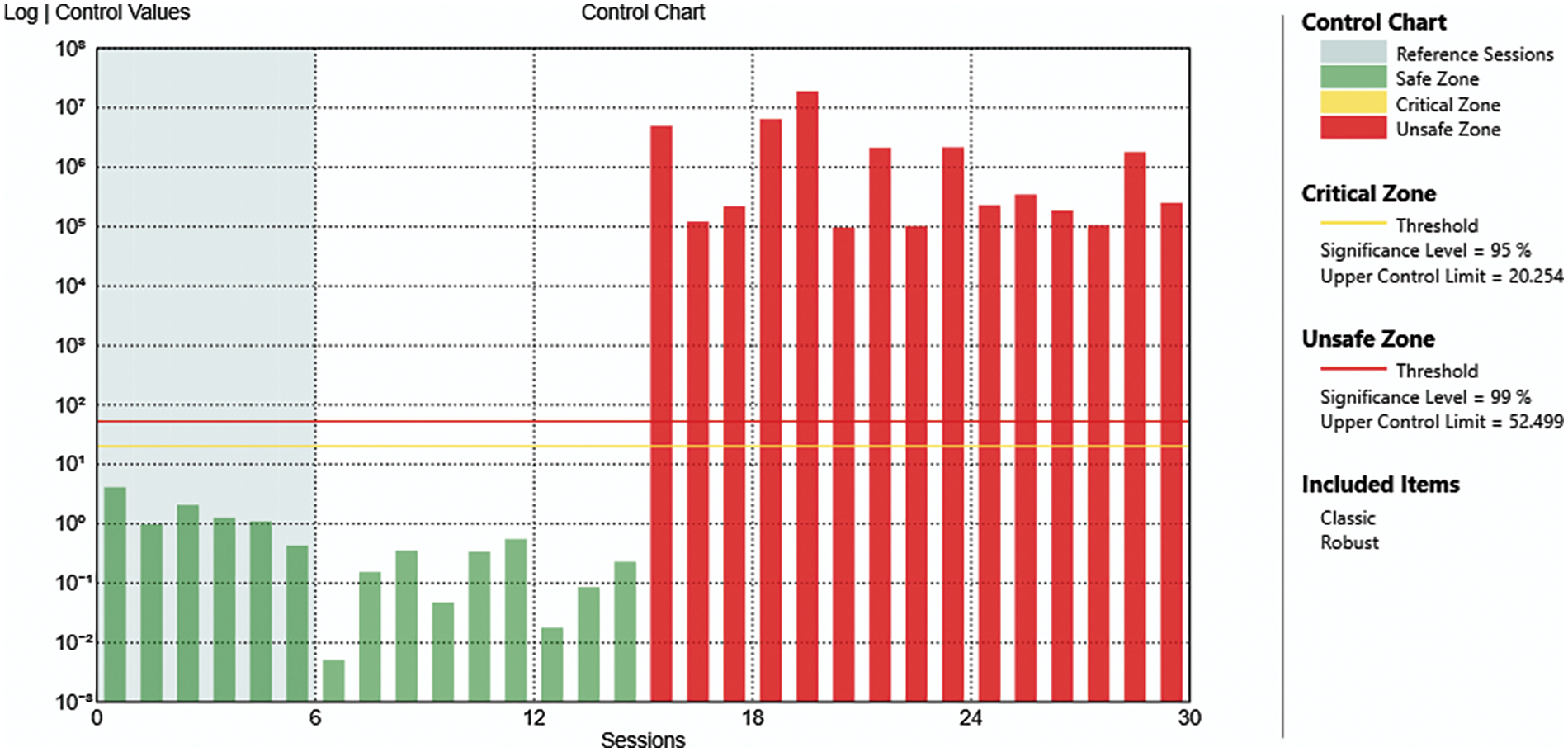
Figure 8: Control chart of the case of damage at level 6 with all mechanisms removed
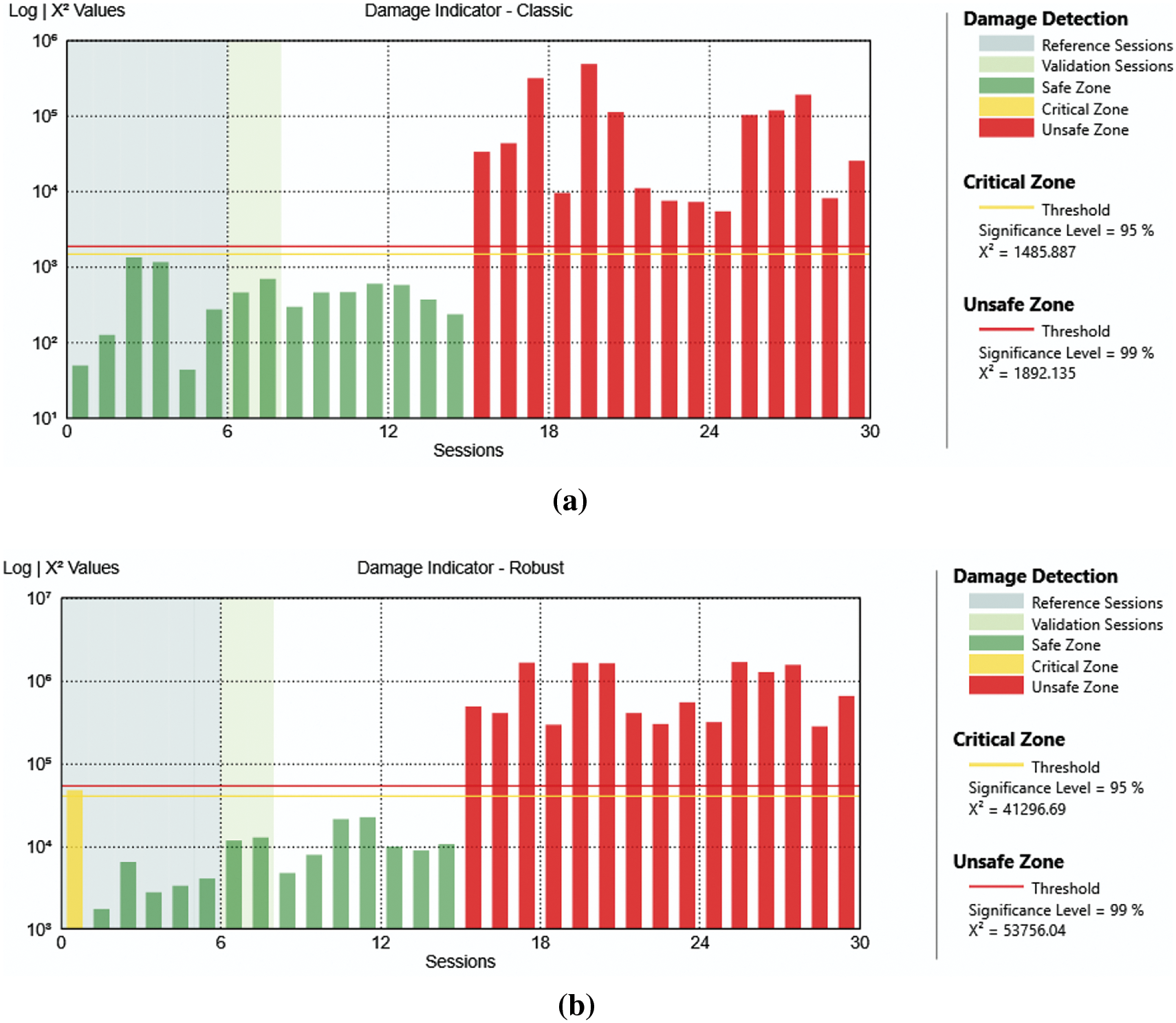
Figure 9: Analysis result of the case with damage at level 4 all mechanisms removed with classic algorithm (a) and robust algorithm (b)
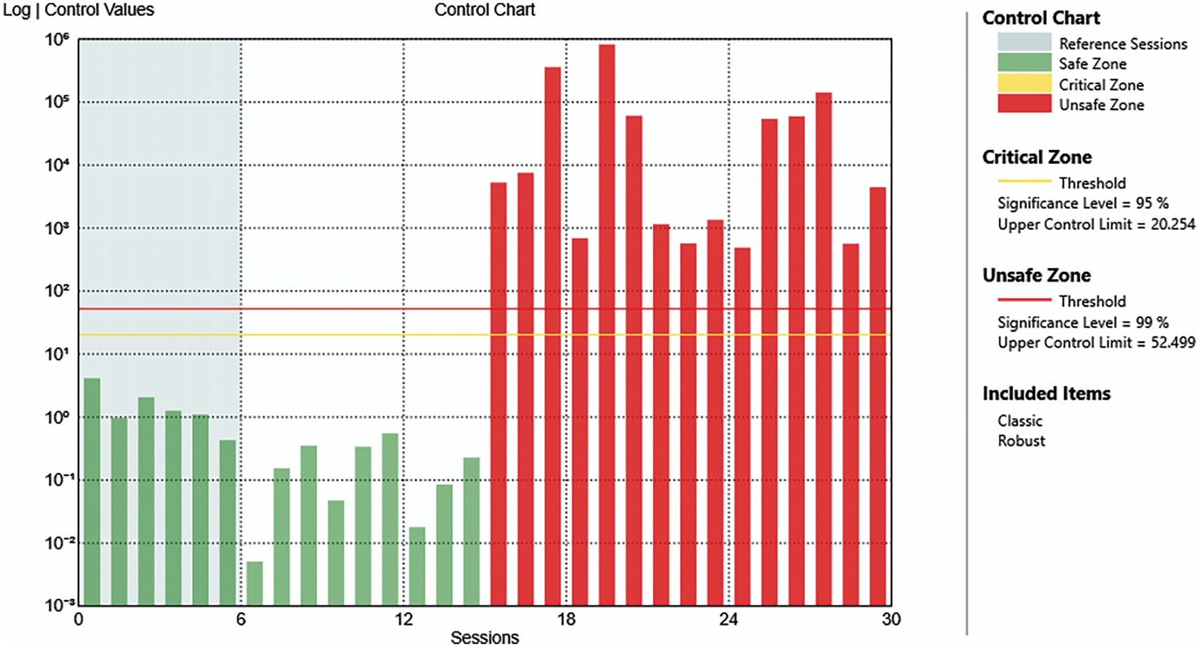
Figure 10: Control chart of the case of damage at level 4 with all mechanisms removed
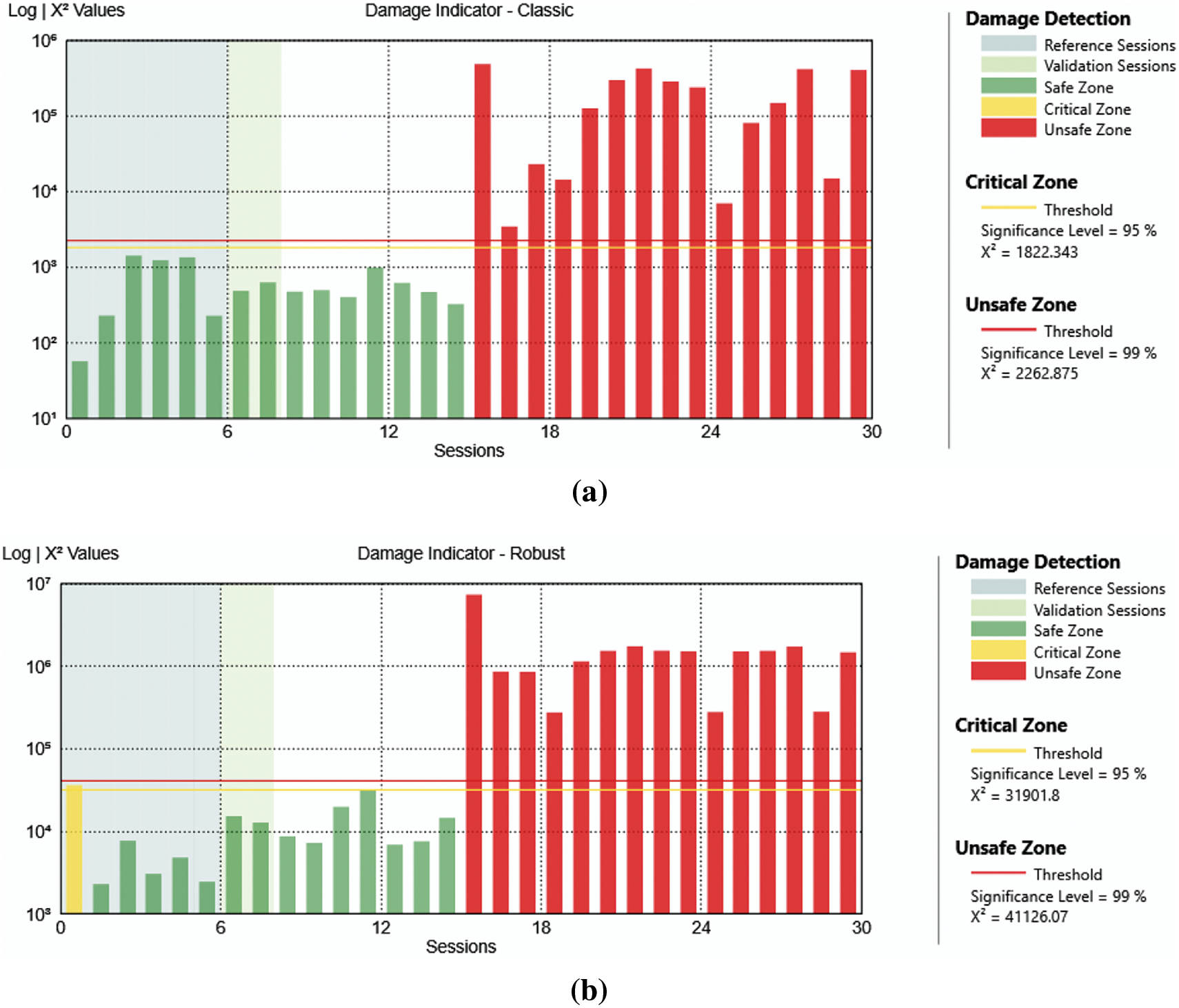
Figure 11: Analysis result of the case with damage at level 3 all mechanisms removed with classic algorithm (a) and robust algorithm (b)
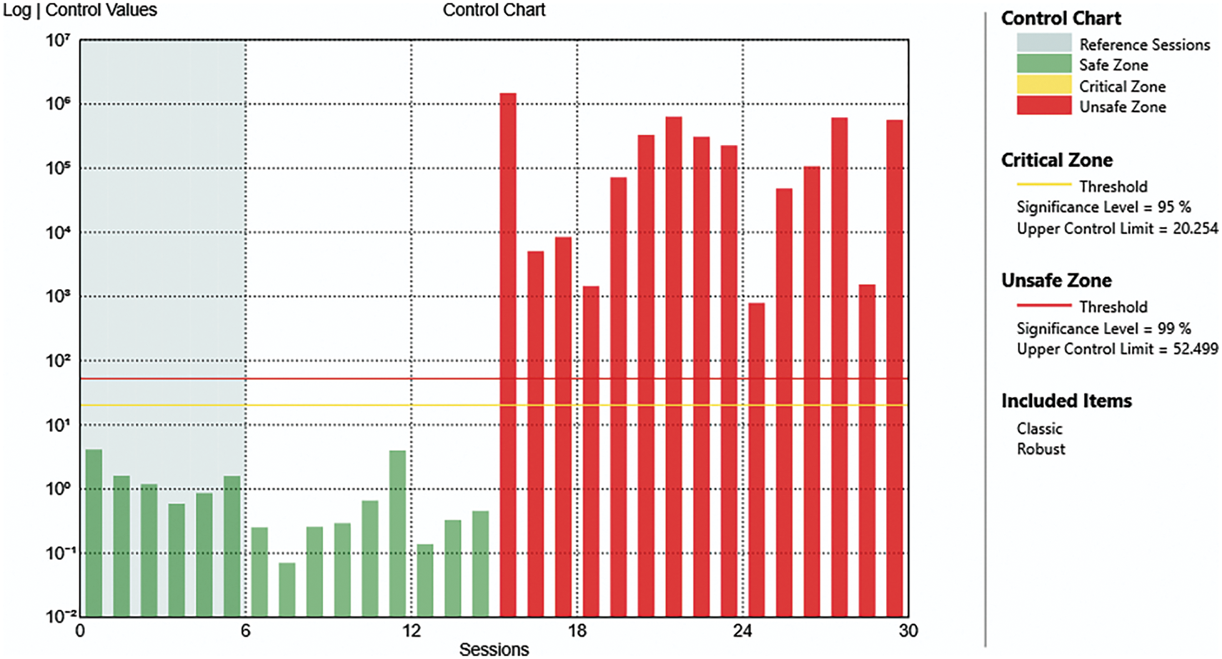
Figure 12: Control chart of the case of damage at level 3 with all mechanisms removed
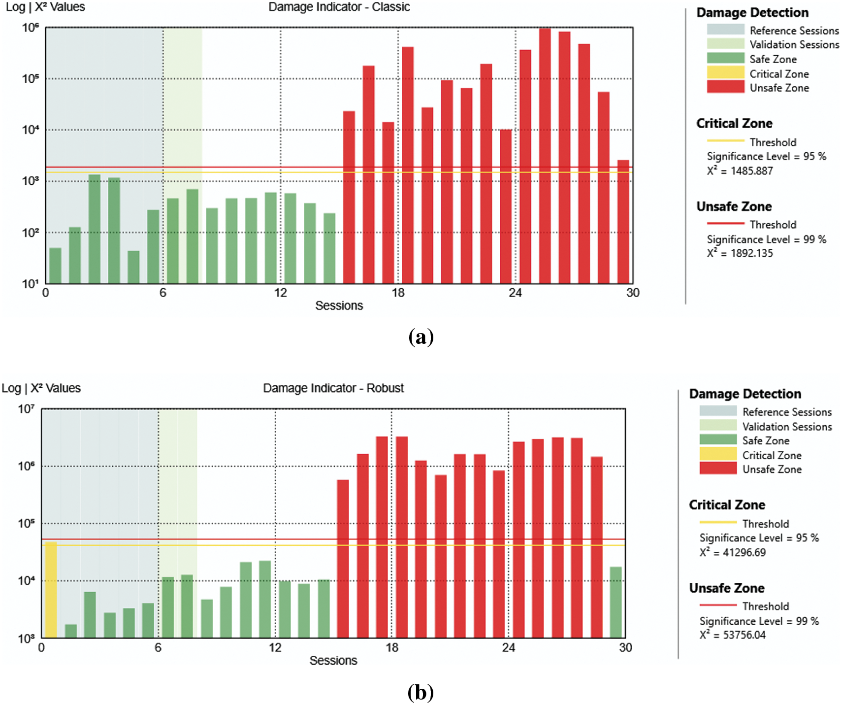
Figure 13: Analysis result of the case with damage at level 6 only one mechanism removed with classic algorithm (a) and robust algorithm (b)
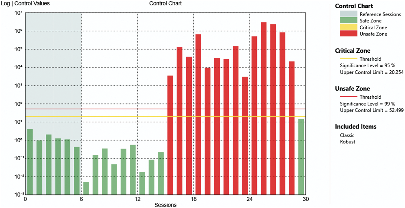
Figure 14: Control chart of the case of damage at level 6 with only one mechanism removed
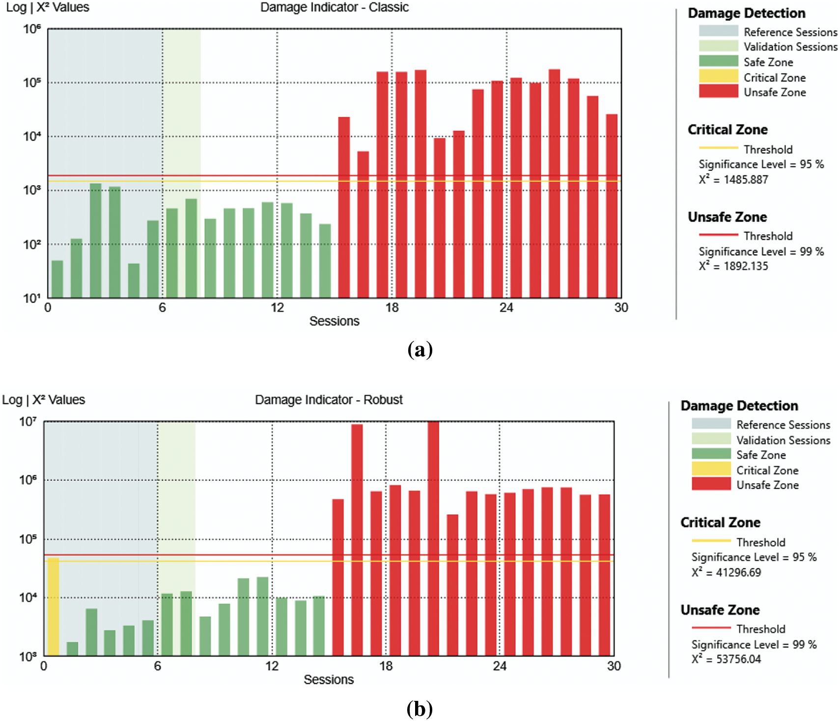
Figure 15: Analysis result of the case with damage at level 4 only one mechanism removed with classic algorithm (a) and robust algorithm (b)
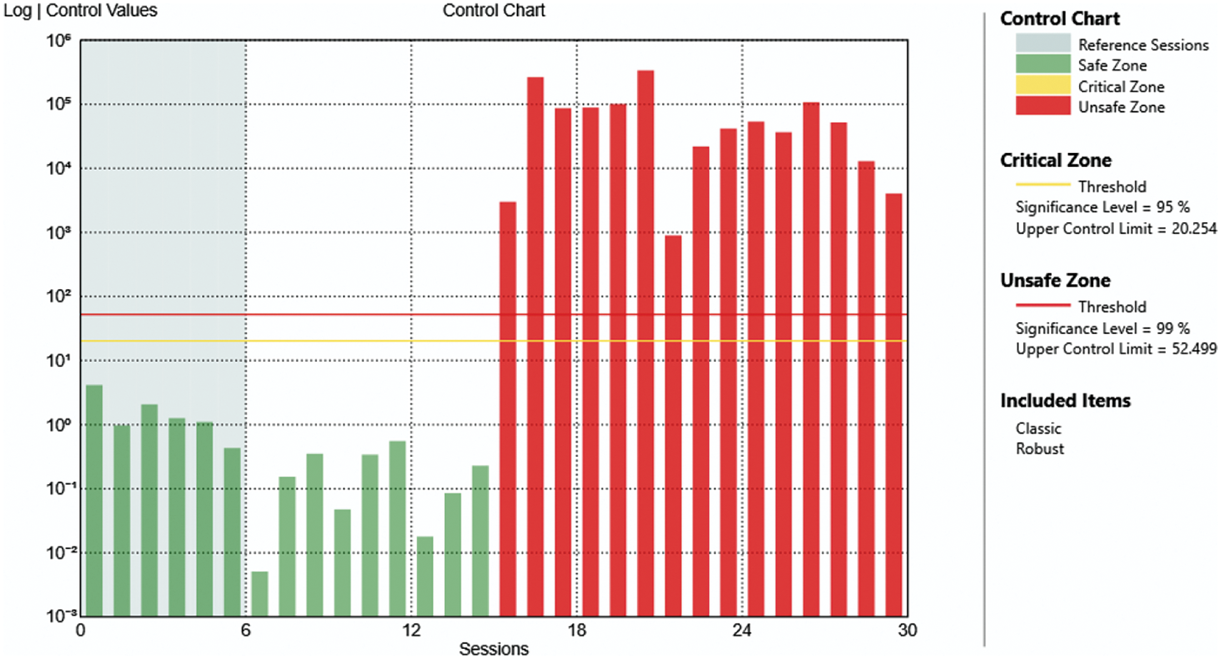
Figure 16: Control chart of the case of damage at level 4 with only one mechanism removed
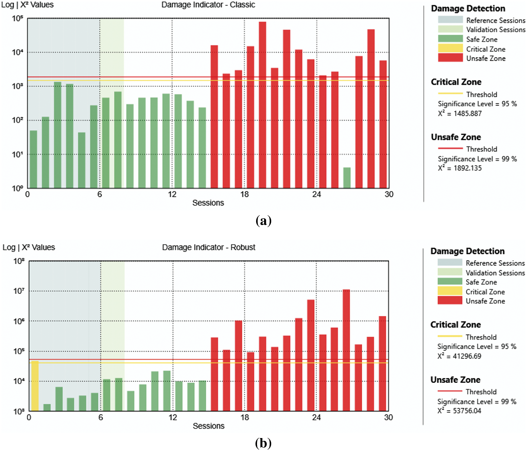
Figure 17: Analysis result of the case with damage at level 3 only one mechanism removed with classic algorithm (a) and robust algorithm (b)
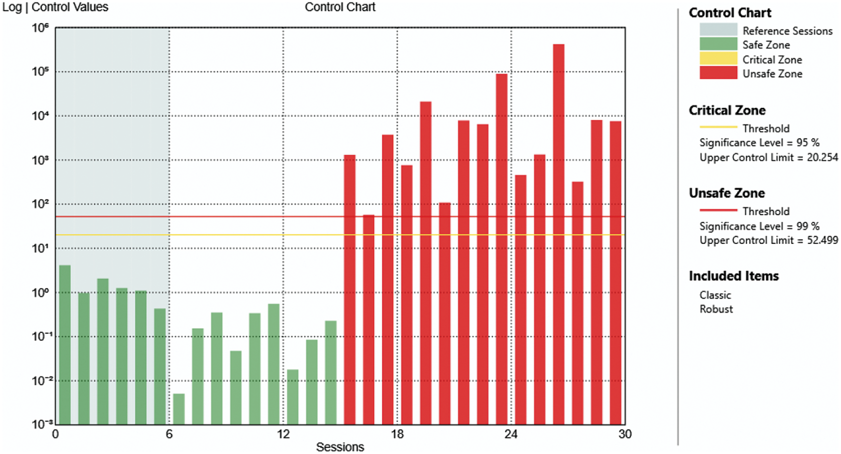
Figure 18: Control chart of the case of damage at level 3 with only one mechanism removed
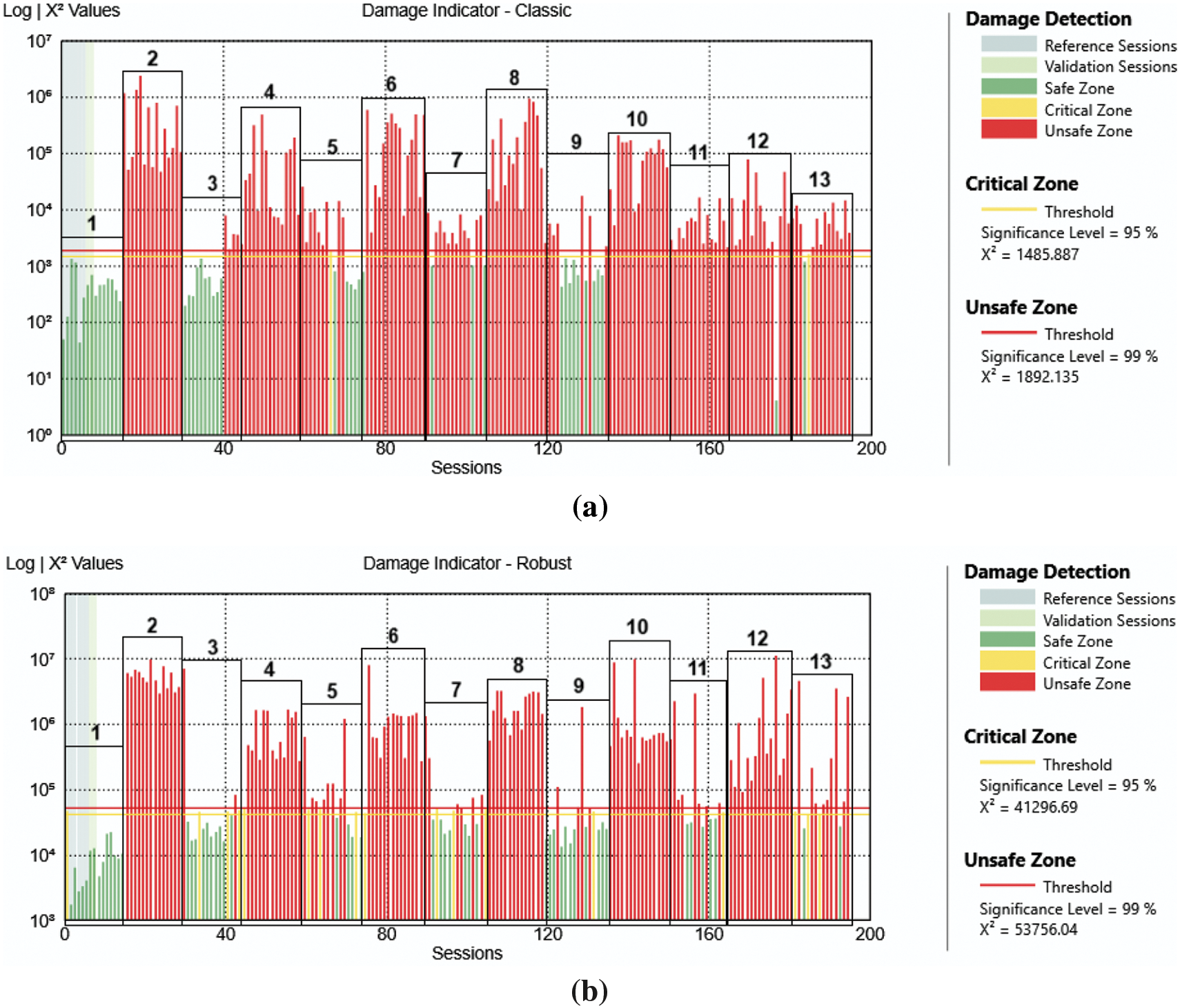
Figure 19: Analysis result of all cases (from period 1 to period 13) with classic algorithm (a) and robust algorithm (b)
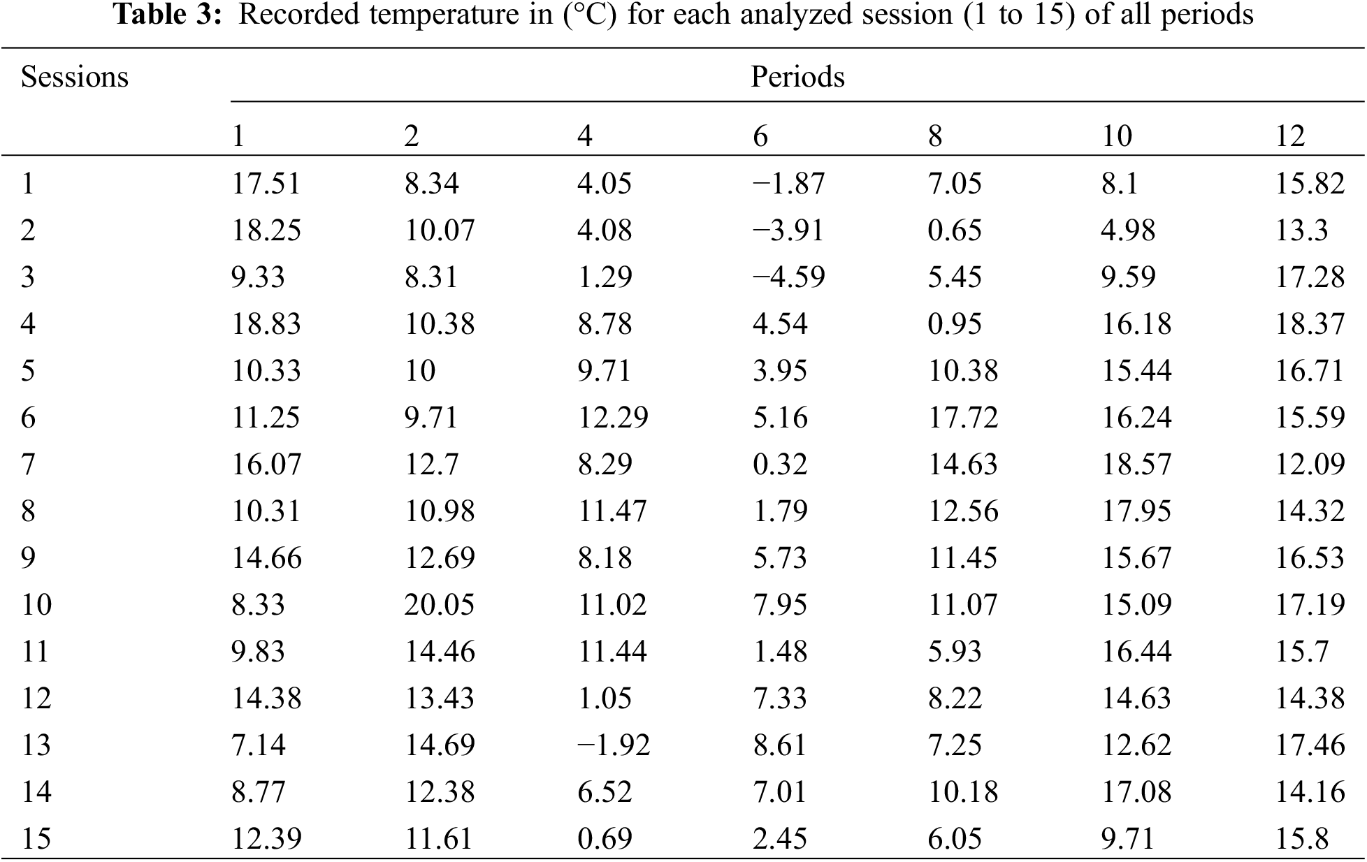
Table 3 displays the recorded temperature for each healthy and damaged session analyzed. There is significant variability across all sessions (1 to 15 for each considered period outlined in Table 2), because they are referred to different times in different period of the year of the acquisition process.
As mentioned before, in Figs. 7–12, the results related to more substantial damage (periods 2, 4, and 6 in Table 2) are displayed, followed by those related to less pronounced damage in Figs. 13–18 (periods 8, 10, and 12 in Table 2). But first, Fig. 5 provides an example of the frequencies related to the first damage that occurred (period 2).
Observing Fig. 5, the blue dots represent the frequency value found for each analyzed session (visible on the x axis), while the average line (continuous line) indicates the modes tracked by the algorithm, connecting the dots related to the frequency belonging to the same vibration mode (for clarity the average line is depicted in Fig. 5 for modes 1, 2 and 5 only). Hence, considering the first five natural frequencies of the truss structure, according to what has been found by the software algorithm, emerges that: the first and the second frequencies, respectively equal to 2.76 and 2.81 Hz, are not sensitive to the presence of the damage, in fact they almost show no changes among all the sessions (shifting from 2.76 to 2.74 Hz the first frequency, and from 2.81 to 2.78 Hz the second one). On the contrary, the third, fourth, and fifth ones, respectively equal to 13.41, 15.93, and 16.28 Hz, show a change on their values starting from the 16th session (the first of the damaged state). This shift is evident from the blue dots, showing that the third frequency goes from 13.42 to 11.64 Hz, the fourth frequency from 15.94 to 14.3 Hz, and the fifth frequency from 16.29 to 14.69 Hz (for the third and fourth frequencies, the dots after the initial damaged session, the 16th session, appear light blue instead of dark blue, indicating that the software was unable to track the relative mode after the damage). For clarity, Fig. 6 provides a zoom on the first two frequencies and the subsequent three.
The software uses the SSI-UPCX algorithm to evaluate the frequencies, and Figs. 5 and 6 can be seen as proof of the sensitivity of some of the natural frequencies of the structure to the damage, which the software is able to evaluate. However, the same change in the third, fourth, and fifth frequencies is not evident for the other types of considered damage. Frequencies are not sensitive in the same way to different types of damage. Structures excited by ambient vibration can also be influenced by changes that naturally occur in the surrounding environment during days and seasons. Therefore, the data collected by the University of Hannover has been tested using the residual method described in Section 2 to assess the state of damage.
The graphical representation of the results obtained with this method (e.g., Fig. 7) is constructed in a simple and intuitive manner. The χ2 values, calculated as explained in Section 2, are depicted: in green if the structure is in a safe condition, in yellow if the structure is in a critical situation, and in red if it is in an unsafe condition, indicating that damage has occurred. The bars turn yellow or red if they exceed the critical or unsafe estimated thresholds, respectively set to the 95th percentile and 99th percentile. These thresholds depend on the reference state model, to which each damaged state data must be compared. This reference state model has been constructed from an average of Hankel matrices of covariance information from a series of reference measurements (sessions). In this case, the reference sessions considered are those related to the first healthy condition (period 1 in Table 2), specifically utilizing data collected during August and September 2020 (it has been tested that the choice of the healthy reference sessions does not influence a lot the results of the damage detection algorithm).
For the residual method, among the 15 sessions related to the healthy state, 8 of these have been used to create the reference state model, as explained above, then 7 more sessions (which are the same for each analysis) from the healthy state have been considered before moving on to analyze the 15 from the damaged state.
The first analyzed case is displayed in Fig. 7. It concerns the case of damage that occurred at level 6 (DAM6) with all mechanisms removed, so data collected during period 2 is considered, and utilized as input for both the classic and robust subspace-based residual algorithms.
In both cases, the obtained results agree with the real condition of the structure in the analyzed data; in fact, the bars related to the first 15 sessions (which correspond to the healthy state) are green, while the bars related to the second 15 sessions (which correspond to damaged state) are red. Only in the robust algorithm, the χ2 value resulting from the first session overcomes the critical threshold, but not the unsafe one; however, this is not a real problem because all the subsequent sessions have given a correct outcome.
Moreover, the information obtained from multiple algorithms can be merged, by the software algorithm, into what is called a “control chart” to reduce the probability of false alarms and to achieve the best possible outcome. This new graph is shown in Fig. 8 for the same case just analyzed in Fig. 7.
As can be seen from Fig. 8, the graph obtained by merging the two in Fig. 7 does not show the critical value in the first session of the “damage indicator-robust” graph anymore, and it appears with more compact values.
In Fig. 9, the result obtained from the comparison of the damage state at level 4 (DAM4) of the structure, with all mechanisms removed (data collected from period 4 in Table 2), against the healthy state of period 1 is displayed.
In Fig. 10, the control chart of the results for the case displayed in Fig. 9 is shown.
Comparing the data relative to the damage that occurred at level 4 with all mechanisms removed, with the healthy state of period 1, the obtained results agree with the real condition of the structure, as the values overcome the unsafe zone threshold only starting from the 16th session; this is even clearer with the control chart in Fig. 10.
Fig. 11 displays the outcome of the case with the damage on level 3 (DAM3) of the structure with all mechanisms removed, so utilizing data collected from period 6. Fig. 12 shows the related control chart.
These results demonstrate that it is possible to correctly evaluate the presence of damage even if it is located in the upper portion of the structure.
The results shown in Figs. 13, 15, and 17, are referred respectively to the same level of damage of Figs. 7, 9, and 11 but only with one mechanism removed per level, i.e., using the data collected in periods 8, 10, and 12 (see Table 2).
From Figs. 12–18, it is clear that it is possible to identify the presence of the damage even if it is less noticeable.
Moreover, the structure has been equipped with reversible damage mechanisms [28]; so, each damage dataset has been spaced out with datasets referred to a reconstructed healthy condition of the structure, as can be seen in Table 2 from periods 3, 5, 7, 9, 11, and 13. In this study, these datasets of healthy conditions have also been examined alongside the damaged ones, utilizing the ARTeMIS Modal software, and the results are depicted in Fig. 19, highlighting each state with the respective period number.
As observed in Fig. 19, the damaged states (periods 2, 4, 6 with all mechanisms removed and 8, 10, 12 with only one bar removed) have consistently been correctly identified, while the healthy states have been accurately identified only in the first period and not in the subsequent ones. This could be ascribed to the damage mechanism, which may have been unsuitable to simulate a real healthy state after the occurrence of damage. As a result, the software algorithms failed to correctly identify the healthy state in comparison to what occurred during the damaged periods.
The present study has verified the possibility of detecting the health status of a real-world structure by monitoring its dynamic behavior through accelerometers placed on the structure itself and using new data processing methodologies.
To concretely evaluate the performance of a damage detection procedure is necessary to test it on a real structure with associated ambient influences, in real-life applications. Regrettably, such tests are exceedingly infrequent, typically with brief campaigns that fail to capture significant environmental variations, and usually cannot be replicated as the investigations end with the demolition of the structures. To address these problems, the present study has taken advantage of the work carried out by the research group of the Leibniz University Hannover which has presented a new database that could be considered a real-life benchmark for vibration-based SHM [28]; such a real-life structure comprises a lattice mast that features a reasonable degree of complexity, it is located outdoors hence exposed to variable environmental conditions and allows the evaluation of several types of damage at different point of the structure.
In this work, this new database, has been utilized to conduct damage detection with the support of a specific software algorithm, the SHM tool of ARTeMIS Modal software that uses methodologies based on subspace decomposition and residual evaluation.
What has emerged is that the examined structure exhibits damages on different levels. It’s possible to identify both the damages obtained by removing all the transversal bracings at a certain level and those obtained by removing only one of them as well. On the other hand, the algorithm has not been able to recognize the intermediate healthy states among the damaged ones, this could be probably due to the reversible damage mechanism used on the structure.
In any case, one of the advantages of this type of algorithm, which arises from the study conducted, as well as insensitivity to changing environmental conditions, is that only a few sessions, and thus only a few minutes of measurement acquisition, are needed to obtain reliable identification of the presence of damage.
Future research aims to assess the localization of damages on the structure, besides their presence identification.
Acknowledgement: None.
Funding Statement: The author N. I. Giannoccaro received funds from the Department of Innovation Engineering, University of Salento, for acquiring the tool Structural Health Monitoring.
Author Contributions: The authors confirm their contribution to the paper as follows: study conception and design: G. F., A. V. D., N. I. G., A. M.; data collection: G. F., A. V. D.; analysis and interpretation of results: G. F., N. I. G. draft manuscript preparation: G. F. All authors reviewed the results and approved the final version of the manuscript.
Availability of Data and Materials: The data used are available on a database as explained in the manuscript.
Ethics Approval: Not applicable.
Conflicts of Interest: The authors declare that they have no conflicts of interest to report regarding the present study.
References
1. Hasani H, Freddi F. Operational modal analysis on bridges: a comprehensive review. Infrastructures. 2023;8(12):172. doi:10.3390/infrastructures8120172. [Google Scholar] [CrossRef]
2. Mishra M, Lourenço PB, Ramana GV. Structural health monitoring of civil engineering structures by using the internet of things: a review. J Build Eng. 2022;48:103954. doi:10.1016/j.jobe.2021.103954. [Google Scholar] [CrossRef]
3. Farrar CR, Worden K. An introduction to structural health monitoring. Philos Trans R Soc Math Phys Eng Sci. 2007;365(1851):303–15. [Google Scholar]
4. Williams E, Messina A, Payne B. Frequency-change correlation approach to damage detection. In: Proceedings of the 15th International Modal Analysis Conference; 1997; Orlando, FL, USA, IMAC. p. 652–7. [Google Scholar]
5. Cárdenas EM, Medina LU. Non-parametric operational modal analysis methods in frequency domain: a systematic review. Int J Eng Technol Innov. 2021;11(1):34–44. doi:10.46604/ijeti.2021.6126. [Google Scholar] [CrossRef]
6. Lorenzo ED, Petrone G, Manzato S, Peeters B, Desmet W, Marulo F. Damage detection in wind turbine blades by using operational modal analysis. Struct Health Monit. 2016;15(3):289–301. doi:10.1177/1475921716642748. [Google Scholar] [CrossRef]
7. Devriendt C, Magalhães F, Weijtjens W, de Sitter G, Cunha Á, Guillaume P. Structural health monitoring of offshore wind turbines using automated operational modal analysis. Struct Health Monit. 2014;13(6):644–59. doi:10.1177/1475921714556568. [Google Scholar] [CrossRef]
8. Pacheco-Chérrez J, Cárdenas D, Delgado-Gutiérrez A, Probst O. Operational modal analysis for damage detection in a rotating wind turbine blade in the presence of measurement noise. Compos Struct. 2023;321:117298. doi:10.1016/j.compstruct.2023.117298. [Google Scholar] [CrossRef]
9. Farrar CR, Doebling SW, Nix DA. Vibration-based structural damage identification. Philos Trans R Soc Lond Ser Math Phys Eng Sci. 2001;359(1778):13149. [Google Scholar]
10. Rainieri C, Notarangelo MA, Fabbrocino G. Experiences of dynamic identification and monitoring of bridges in serviceability conditions and after hazardous events. Infrastructures. 2020;5(10):86. doi:10.3390/infrastructures5100086. [Google Scholar] [CrossRef]
11. Azim MR, Gül M. Damage detection of steel girder railway bridges utilizing operational vibration response. Struct Control Health Monit. 2019;26(11). doi:10.1002/stc.2447. [Google Scholar] [CrossRef]
12. Magalhães F, Cunha A, Caetano E. Vibration-based structural health monitoring of an arch bridge: from automated OMA to damage detection. Mech Syst Signal Process. 2012;28:212–28. doi:10.1016/j.ymssp.2011.06.011. [Google Scholar] [CrossRef]
13. ARTeMIS Modal. Structural vibration solutions. Available from: https://www.svibs.com/artemis-modal/. [Accessed 2024]. [Google Scholar]
14. Rytter A. Vibration-based inspection of civil engineering structures (Ph.D. Thesis). Aalborg University: Denmark; 1993. [Google Scholar]
15. Diaferio M, Foti D, Mongelli M, Giannoccaro NI, Andersen P. Operational modal analysis of a historic tower in bari. In: Proulx T, editor. Civil engineering topics. New York, NY: Springer New York; 2011. vol. 4, p. 335–42. [Google Scholar]
16. Jimenez Capilla JA, Au SK, Brownjohn JMW, Hudson E. Ambient vibration testing and operational modal analysis of monopole telecoms structures. J Civ Struct Health Monit. 2021;11(4):1077–91. doi:10.1007/s13349-021-00499-4. [Google Scholar] [CrossRef]
17. Gres S, Andersen P, Damkilde L. Operational modal analysis of rotating machinery. In: di Maio D, editor. Rotating machinery, vibro-acoustics & laser vibrometry. Cham: Springer International Publishing; 2019. vol. 7, p. 6775. [Google Scholar]
18. Silva MS, Neves FA. Modal identification of Bridge 44 of the Carajás Railroad and numerical modeling using the finite element method. Rev IBRACON Estrut E Mater. 2020;13(1):39–68. doi:10.1590/s1983-41952020000100005. [Google Scholar] [CrossRef]
19. Rosenow SE, Andersen P. Operational modal analysis of a wind turbine mainframe using crystal clear SSI. In: Proulx T, editor. Structural dynamics and renewable energy. New York, NY: Springer New York; 2011. vol. 1, p. 153–62. [Google Scholar]
20. Jacobsen NJ, Andersen P, Mendler A, Gres S. A general framework for damage detection with statistical distance measures: application to civil engineering structures. In: 9th International Operational Modal Analysis Conference; 2022 Jul 3–6; Vancouver, Canada. [Google Scholar]
21. Gres S, Ulriksen MD, Döhler M, Johansen RJ, Andersen P, Damkilde L, et al. Statistical methods for damage detection applied to civil structures. Procedia Eng. 2017;199:1919–24. doi:10.1016/j.proeng.2017.09.280. [Google Scholar] [CrossRef]
22. Ventura C, Andersen P, Mevel L, Döhler M. Structural health monitoring of the Pitt River Bridge in British Columbia, Canada. In: WCSCM-6th World Conference on Structural Control and Monitoring; 2014 Jul; Barcelona, Spain. [Google Scholar]
23. Kaloop MR, Hu JW. Stayed-cable bridge damage detection and localization based on accelerometer health monitoring measurements. Shock Vib. 2015;2015:1–11. doi:10.1155/2015/102680. [Google Scholar] [CrossRef]
24. Lee ET, Rahmatalla S, Eun HC. Damage detection by mixed measurements using accelerometers and strain gages. Smart Mater Struct. 2013 Jul 1;22(7):075014. doi:10.1088/0964-1726/22/7/075014. [Google Scholar] [CrossRef]
25. Nabavi S, Gholampour S, Haji MS. Damage detection in frame elements using Grasshopper Optimization Algorithm (GOA) and time-domain responses of the structure. Evol Syst. 2022 Apr;13(2):307–18. doi:10.1007/s12530-021-09389-y. [Google Scholar] [CrossRef]
26. Fallahian S, Joghataie A, Kazemi MT. Structural damage detection using time domain responses and teaching-learning-based optimization (TLBO) algorithm. Sci Iran. 2017 Aug 19. doi:10.24200/sci.2017.4238. [Google Scholar] [CrossRef]
27. Barthorpe RJ, Manson G, Worden K. On multi-site damage identification using single-site training data. J Sound Vib. 2017 Nov;409:43–64. doi:10.1016/j.jsv.2017.07.038. [Google Scholar] [CrossRef]
28. Wernitz S, Hofmeister B, Jonscher C, Grießmann T, Raimund R. A new open-database benchmark structure for vibration-based Structural Health. Struct Control Health Monit. 2022;29(11):e3077. doi:10.1002/stc.3077. [Google Scholar] [CrossRef]
29. Jonscher C, Hofmeister B, Grießmann T, Rolfes R. Influence of environmental conditions and damage on closely spaced modes. In: Rizzo P, Milazzo A, editors. European workshop on structural health monitoring. Cham: Springer International Publishing; 2023. p. 902–11. [Google Scholar]
30. Möller S, Jonscher C, Grießmann T, Rolfes R. Investigations towards physics-informed gaussian process regression for the estimation of modal parameters of a lattice tower under environmental conditions. In: Limongelli MP, Giordano PF, Quqa S, Gentile C, Cigada A, editors. Experimental vibration analysis for civil engineering structures. Cham: Springer Nature Switzerland; 2023. vol. 433, p. 401–10. doi:10.1007/978-3-031-39117-0. [Google Scholar] [CrossRef]
31. Römgens N, Abbassi A, Jonscher C, Grießmann T, Rolfes R. Unsupervised damage localization using autoencoders with time-series data. In: Limongelli MP, Giordano PF, Quqa S, Gentile C, Cigada A, editors. Experimental vibration analysis for civil engineering structures. Cham: Springer Nature Switzerland; 2023. p. 511–9. [Google Scholar]
32. Liesecke L, Jonscher C, Grießmann T, Rolfes R. Investigations of mode shapes of closely spaced modes from a lattice tower identified using stochastic subspace identification. In: Limongelli MP, Giordano PF, Quqa S, Gentile C, Cigada A, editors. Experimental vibration analysis for civil engineering structures. Cham: Springer Nature Switzerland; 2023. p. 529–38. [Google Scholar]
33. Wickramarachchi CT, Poole J, Hubler C, Jonscher C, Rolfes R. Statistical alignment in transfer learning to address the repair problem: An experimental case study. Hannover: Institutionelles Repositorium der Leibniz Universität Hannover; 2024. doi:10.15488/16089. [Google Scholar] [CrossRef]
34. Peeters B, De Roeck G. Reference-based stochastic subspace identification for output-only modal analysis. Mech Syst Signal Process. 1999 Nov;13(6):855–78. doi:10.1006/mssp.1999.1249. [Google Scholar] [CrossRef]
35. van Overshee P, de Moor B. Subspace identification for linear systems: Theory-Implementation–Applications. Katholieke Universiteit Leuven Belgium: Kluwer Academic Publishers (Dardrecht Netherlands); 1996. [Google Scholar]
36. Benveniste A, Mevel L. Nonstationary consistency of subspace methods. IEEE Trans Autom Control. 2007 Jun;52(6):974–84. doi:10.1109/TAC.2007.898970. [Google Scholar] [CrossRef]
37. Döhler M, Mevel L. Fast multi-order computation of system matrices in subspace-based system identification. Control Eng Pract. 2012 Sep;20(9):882–94. doi:10.1016/j.conengprac.2012.05.005. [Google Scholar] [CrossRef]
38. Döhler M, Mevel L, Hille F. Subspace-based damage detection under changes in the ambient excitation statistics. Mech Syst Signal Process. 2014 Mar;45(1):207–24. doi:10.1016/j.ymssp.2013.10.023. [Google Scholar] [CrossRef]
Cite This Article
 Copyright © 2024 The Author(s). Published by Tech Science Press.
This work is licensed under a Creative Commons Attribution 4.0 International License , which permits unrestricted use, distribution, and reproduction in any medium, provided the original work is properly cited.
 Downloads
 Citation Tools