Time-History Dynamic Characteristics of Reinforced Soil-Retaining Walls

1  Introduction

Reinforced earth retaining walls are frequently utilized in civil engineering [1], such as highways and railroads in seismically active locations, due to their excellent technical performance and economic benefits. Reinforced soil retaining walls are normally made out of panels, fill, and reinforcement. Previous earthquake catastrophe instances indicate that reinforced earth retaining walls function better seismically. For example, Huang [2] and Ling et al. [3] discovered that, except certain reinforced earth retaining walls with too high vertical spacing of reinforcing materials, which caused local panel damage, other walls did not sustain major damage during the Ji-ji earthquake in Taiwan. A 10 m high reinforced earth retaining wall, which was similarly impacted by the 1999 Kocaeli earthquake (M7.4), showed relatively moderate residual deformation [4]. In contrast to the widespread collapse of other types of retaining structures during the EL Salvador earthquake, the reinforced earth retaining wall sustained little damage. All nations have developed design guidelines to guide the construction of reinforced earth retaining walls under earthquake loads. The seismic design of reinforced earth retaining wall primarily consists of determining ground pressure and calculating stability, with the latter often using the M-0 or S-W methods [5]. Although the design code provides reference and guidance for the design of reinforced soil retaining walls under earthquake load, numerous research findings show that the pseudo-static method cannot accurately explain the dynamic response of reinforced soil retaining walls under earthquake action, and it frequently leads to overly conservative design [6]. For example, El-Emam et al. [7] found that the toe of the wall bore nearly 50% of the earth pressure through a shaking table test; Vieira et al. [8] believed that equating instantaneous and short-term seismic loads to constant loads would cause the calculated earth pressure coefficient to be too large. Athanasopoulos-Zekkos et al. [9] found that earth pressure and inertial force did not act synchronously on the wall. At the same time, based on a shaking table test, Tatsuoka [10] found that the dynamic earth pressure of the wall under earthquake load did not increase, and even appeared to be less than the initial earth pressure.

The shaking table test is the most direct research tool for studying the reaction mechanism of reinforced soil retaining walls during an earthquake [11]. Although the shaking table test can directly measure the stress and strain of the research item and see the entire failure process, the research cost is considerable, and many factors such as test model accuracy and parameter setting will impact the accuracy of the test findings. Dynamic time history analysis is a kind of numerical analysis method. It adopts elastic and elastic-plastic constitutive models of the research object to simulate the stress and deformation process of the research object under external loads. Compared with the shaking table test, the research cost of the numerical analysis method is relatively low, and it can also facilitate parameter research [12–15]. In this study, the reinforced soil composite material is regarded as a kind of structural form that can consider the sliding between reinforcement and soil mass. The finite element calculation program of composite response analysis is developed. The vibration time history of the reinforced earth retaining wall is calculated, and the vibration process characteristics of the reinforced earth retaining wall are obtained and compared with the gravity retaining wall. The dynamic response characteristics of the reinforced earth retaining wall are analyzed, which provides technical support for the seismic design of the retaining wall structure.

2  Reinforcement-Soil Slip Constitutive Model

Because of the complexity of the calculation and the difficulty in defining the calculation parameters, the dynamic elastoplastic approach has not been completely used in the calculation of soil dynamic response. In the dynamic computation of soil, the composite response analysis approach is extensively utilized. The complicated stiffness matrix of the reinforced soil composite material should be determined when the composite response analysis method is employed to calculate the reinforced soil retaining wall. [K*] is the element stiffness matrix composed of complex modulus, expressed as

[K∗]=[K](1−2λ2+i2λ1−λ2) (1)

Two parameters need to be determined in the formula, the real stiffness matrix can be calculated by the general finite element method, and stiffness matrix calculation needs to determine the constitutive model of the reinforced soil composite material, the damping ratio is more complicated, and need to be iterated by equivalent linearization method.

2.1 Reinforced Soil Composite Considering Slip

It is found in the test that the sliding surface between reinforcement and soil is not on the reinforcement surface, but in the soil which is a certain distance away from the reinforcement surface [16]. This indicates that a part of the soil around the upper and lower parts of the reinforcement will slide together with the reinforcement in the event of slippage, and it can be considered that the soil in a certain range above and below the reinforcement and the reinforcement form a shear zone. In this paper, the reinforcement and the upper and lower parts of the soil are regarded as a shear zone and the reinforcement element, and the elements outside the shear zone are regarded as the soil element.

As shown in Fig. 1, reinforcement and soil are connected through shear bands interacting around reinforcement, and the proportion of reinforcement in the section is

a=BtBT=tT (2)

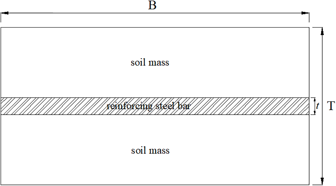
Figure 1: Reinforced-soil composite unit

By assigning appropriate stiffness to the shear zone, the deformation of the reinforcement relative to the soil matrix can be small. The elastic analysis can be used, and the Mohr Coulomb criterion can be used to limit the shear stress of the soil in the slip analysis.

2.2 Strain-Displacement Relationship

In Fig. 2, Point P0 represents the initial position of the research point in the reinforced soil composite material. After deformation, it moves to Point P in the soil and Point P* in the reinforcement, and SS represents the direction of the reinforcement material. Therefore, the calculation model only allows the reinforcement to displace relative to the soil in the horizontal direction, that is, PP* is approximately parallel to SS. This approximation is due to geometric changes due to strain, which are generally assumed to be minor, so that PP* and SS can be considered parallel.

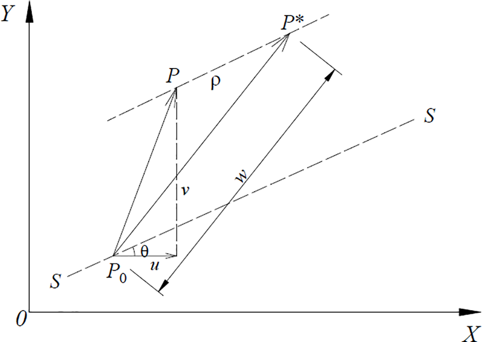
Figure 2: The motion of the bar point

The longitudinal strain εs of the reinforcement is the gradient of the total displacement w of a point on the reinforcement along the SS direction. The following relation can be obtained from the geometric figure in Fig. 2.

w=uαx+vαy+ρ (3)

where αx=cos⁡θ,αy=sin⁡θ , therefore, the following relationship can be obtained:

εs=dwds=αxduds+αydyds+dρds (4)

By considering the spatial variation of w, u, v, and ρ, the derivative of the variable can be expanded by the chain rule as follows: let δ=δ(x,y) represent u, v, or ρ, then

dδds=αxdδdx+αydδdy (5)

Substituting u, v and ρ into δ , the strain formula can be expressed as

εs=αx2∂u∂x+αy2dvdy+αxαy(∂u∂y+∂v∂x)+αx∂ρ∂x+αy∂ρ∂y (6)

The shear strain in the shear zone is expressed by the following formula:

γs=ρB (7)

The displacement component of soil is related to u and v, which is expressed by the following relation:

εx=∂u∂xεy=∂v∂yγ=∂u∂y+∂v∂x} (8)

In addition to u and v, the relative displacement p of reinforcement to soil is selected as the node variable.

2.3 Element Stiffness Matrix

The stiffness matrix of a stiff-soil composite material is divided into two parts: the soil stiffness contribution and the shear zone stiffness contribution. When n is used to denote an element’s node number, the composite stiffness matrix is of 3 n order. As a result, the combined component matrix is of 3 n order, and the composite element stiffness matrix may be represented as

K=K1+K2 (9)

where K1 and K2 are matrix components of soil mass and shear zone, respectively. Using the principle of virtual work, both component matrices can be expressed as

Ki=∫BiTDiBidxdydz (10)

The soil stiffness matrix B1 is obtained from the discrete formula, using the standard form of the plane strain problem. The difference is that a column of zeros needs to be inserted every three columns, so that the order of the matrix is 3 × 3 n, and B1 is composed of a column of B1i (i = 1, …, n) form submatrices.

B1i=[∂Ni∂x000∂Ni∂i0∂Ni∂y∂Ni∂x0] (11)

where Ni is the form function of node i. D is a plane strain matrix of order 3 × 3, i.e.,

D1=E(1−v)(1+v)(1−2v)[1v1−v0v1−v10001−2v2(1−v)] (12)

Matrix B2, εs and γs are related to node variables, and the submatrix of node i obtained by discretization is

B2i=[αxQi0αyQi0QiNi/ε] (13)

Qi=αx∂Ni∂x+αy∂Ni∂y (14)

The modulus matrix D2 connects the normal stress τs , εs and γs of the reinforcement with the shear stress σs of the reinforcement. In order to integrate B2TD2B2 on the soil element, a and Gs are multiplied to obtain Es, which can obtain the integral of the contribution to the longitudinal stiffness of the reinforcement on the volume of the reinforcement and the contribution to the shear stiffness on the volume of the shear band, so D2 is defined as

D2=[aEs00GsB] (15)

As mentioned above, different Gs values can be set in the program for different situation analysis. K2 is given by the formula above, which is

K2ij=aEsQiQj[αx2αxαyαxαxαyαy2αyαxαy1+Rij] (16)

where Rij=GsBaEs(NiNjQiQj) .

By adding the stiffness contribution of the reinforcement shear band to the soil, the total stiffness matrix of the element is obtained. Then conventional finite element analysis is carried out, and the soil strain is calculated from the displacement of the element node.

2.4 Comparison of Examples

McGown et al. [17] investigated the influence of inclusion characteristics and orientation on sand behaviour using a planar strain unit cell device. Tests were carried out on dense medium and loose sand samples with or without inclusions. The materials utilised were Leighton Buzzard sand with particle sizes ranging from 0.4 to 1.0 mm, and all experiments employed a homogeneity coefficient of 1.13. The greatest and minimum porosities of the sand are 0.45 and 0.345, respectively. Three types of inclusions were used: fabric, aluminium foil, and aluminium mesh. The fabric is non-woven, melt-bonded, and made of 25% nylon and 75% polypropylene in the form of 50% polypropylene homo-filaments and 50% polypropylene with nylon sheath hetero-filaments. The tested model dimensions are 152 mm in length, 102 mm in width, and 102 mm in height. Two types of reinforcing materials are being considered: aluminium foil and T140 geotextile. The test is carried out by placing a layer of reinforcing material horizontally in the centre of the model. Fig. 3 depicts the model’s boundary conditions, which include a horizontal pressure of 70 kPa. Geotextile T140 exhibited mild nonlinearity in the tensile test. Its ultimate strength at 18% strain was 3.0 kN/m, which was used as the tensile strength in the model. The average slope of the load-elongation curve was 26.5 kN/m, which was used to determine the stiffness of the reinforcement.

Figure 3: Grid and boundary conditions for plane strain simulation of a layered model

The thickness of the T140 geotextile is 1 mm, and the volume ratio of the reinforcement is χ=0.0098 . In order to calculate the characteristics of the reinforcement applied in the constitutive model of the reinforced soil, the strength parameter given in Table 1 is divided by the thickness, and then multiplied by the volume ratio of the reinforcement. The formula for calculating the elastic modulus of the reinforcement is Er=26.5/0.001×0.0098=259.8 kN/m2 , and the tensile strength of the reinforcement is σr=3.0/0.001×0.0098=29.41 kN/m2 .

Fig. 4a compares the measured performance of the reinforced T140 geotextile specimen with the algorithm in this paper, and it can be found that the calculated value of the peak strength is similar to the experimental value. However, the simulation results show that the reinforcement has more ductility. Due to the low elastic modulus and high extensibility of geotextiles, more strain is needed to reach the peak strength. Fig. 4b shows the effect of reinforcement load on the axial strain of the reinforced sample in the simulation comparison between the algorithm in this paper and the layer model. As shown in the figure, the reinforcement in the algorithm model and the reinforcement in the layer model yield when the strain is about 6.5%.

Figure 4: Comparison of calculation results

At the initial loading stage, the strain of the model is small, and the slip constitutive model of reinforced soil has a good agreement with the McGow test and the layer model, indicating that the displacement of reinforcement in the soil is small in the initial elastic stage. The slip constitutive model of reinforced soil can simulate the stress-strain behavior of the composite with no or little slip of reinforcement. With the increase in loading time, the stiff-soil composite will gradually yield deformation, in which the stiff soil will have a large slip relative to the soil. In this case, there is some gap between the stiff soil slip constitutive model and the numerical results of the McGow test and layer model, but the overall gap is small. As shown in Fig. 4a, at peak strength, the data of the reinforced soil slip constitutive model is close to that of the layer model, but slightly different from the McGow test result. The reason may be that both the reinforced soil slip constitutive model and the layer model are close to each other through numerical calculation, while the accuracy of the McGow test is affected by test conditions.

The calculation of the tensile force of different reinforcement materials can be realized by changing parameters in the program, and the change of the tensile force of reinforcement materials can be obtained by controlling the change of input parameters of reinforcement materials and the calculation parameters of reinforcement elements. As shown in Fig. 4b, the relationship between tensile force and axial strain of reinforcements materials in the bedding model and the slip constitutive model of reinforcement soil is calculated. The results show that, with the increase of the axial strain, the tension of the two reinforcement has a good consistency, but the difference between the two results does not increase due to the small strain, which indicates that the slip constitutive model can better reflect the stress-strain relationship of the reinforced soil composite.

3  Dynamic Finite Element Analysis Program Design

In this paper, the seismic response time history analysis of reinforced soil retaining wall structure is calculated by using the composite response analysis method. The composite response analysis method has been widely used in the field of geotechnical seismic engineering, and the theoretical research is more mature than the elastic-plastic analysis. Especially for the material with high damping such as soil, the composite reaction analysis can avoid the influence of structure frequency independent of damping ratio change and the calculation amount is small.

3.1 Structure and Function of the Program

Fortran has a significant advantage over other languages with its built-in complex number type, which allows it to operate directly on complex numbers. The core of the composite response analysis program lies in the assembly and solution of the complex stiffness matrix. The integral of the element stiffness matrix adopts a general method. According to the calculation formula of the composite stiffness matrix, the real and imaginary parts of the element composite stiffness matrix are assembled first. After the complex stiffness matrix is assembled, the equilibrium equations shown below can be solved.

[M]{u¨}+[K∗]{u}=−[M]{u¨0} (17)

Damping of the advantage of this approach is to introduce a complex stiffness matrix of the equivalent form of the complex stiffness matrix [K*], due to the damping ratio contained in the complex stiffness matrix, can get the amplitude of the damping ratio under the same as the modal analysis, and have the same phase approximation.

Under the linear assumption, the solution of the equations can be obtained by {us}, then using the Fourier inverse transformation step every hour of the displacement can be obtained, this procedure is used to solve continuous media plane strain problem, with eight nodes unit parameters, such as preparation, mass matrix in the form of lumped mass matrix.

3.2 Solving Stiffness Matrix

In practical application, the isoparametric element is widely used. The form function of the isoparametric element is generally established in a reference coordinate system. Through the coordinate transformation of the form function, any quadrilateral or hexahedron in physical space can be converted into a square or cube in the reference coordinate system (see Fig. 5). Because the element of a curved edge or surface can describe the solution region more precisely, and the application of higher order displacement interpolation function has higher precision and is very beneficial to the realization of the program. The formula for calculating the element stiffness of a plane elastomer is

[K]=∫∫[B]T[D][B]dxdy (18)

where [B] is the strain-displacement matrix, [D] is the stress-strain matrix, whose general form can be expressed as follows:

[B]=[Ni,x00Ni,yNi,yNi,x] (19)

Figure 5: Rectangular element and isoparametric element

In the case of plane stress, the strain submatrix is

[S]=[D][B]=E1−μ2[Ni,xμNi,yμNi,x(1−μ)Ni,y/2Ni,y(1−μ)Ni,x/2] (20)

For plane strain, simply replace E with E/(1−μ2) and μ with μ/(1−μ) .

The additional stiffness matrix corresponding to the composite matrix is

[KE]=[K11K12K13K14K21K22K23K24K31K32K33K34K41K42K43K44] (21)

where

[Kij]=∫−11∫−11[Bi]T[E][Bj]|J|dξdη

Gauss-legendre integral method is generally used to integrate the element stiffness into the weighted sum of the function values of the sampling points, and the integral form is

∫−11∫−11f(ξ,η)dξdη≈∑i=1n∑j=1nwiwjf(ξi,ηi) (22)

According to Gauss-Legendre integral method, the numerical integral formula of stiffness matrix of isoparametric element with 4-8 nodes is

Ke=∑i=1n∑j=1nwiwj(BTDB|J|)ij (23)

In the process of finite element solution, the final solution process is a system of equations composed of a stiffness matrix. The compound response analysis belongs to the linear solution, and its solving object is a group of linear equations. The solution of the equations is carried out by the Gaussian elimination method.

4  Dynamic Finite Element Analysis

In dynamic analysis of reinforced soil retaining walls, the vibration propagates to an infinite distance, and the actual research object is half space, but the finite element model can only be bounded, so it is necessary to approximate the boundary conditions of the model. Theoretically, the farther away the boundary position is from the structure, the less seismic waves will be reflected on the boundary and the less the influence of artificial boundary conditions on the seismic dynamic response of the structure. Considering the accuracy and amount of calculation of the model [18,19], the size of the finite element calculation model is shown in Fig. 6.

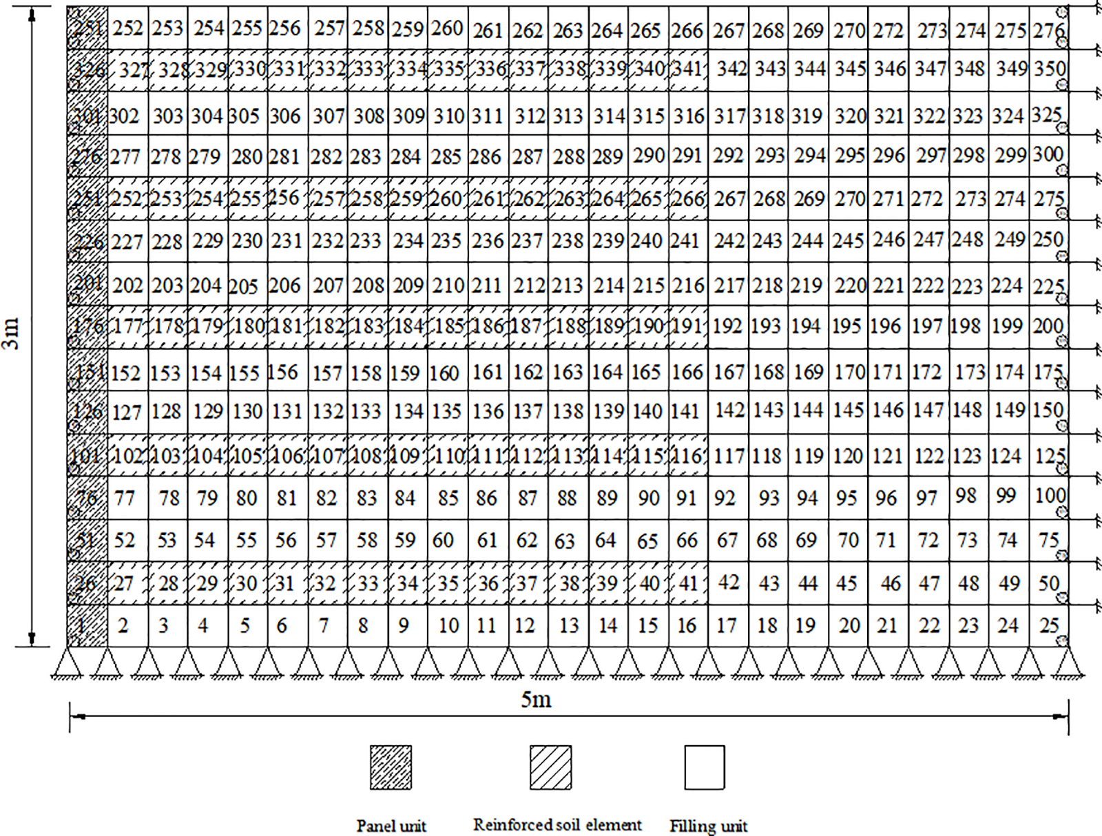
Figure 6: Finite element mesh of reinforced soil retaining wall

The results of finite element calculation are related to the method of unit division. Generally speaking, the more units are divided, the more accurate the calculation results will be. For the reinforced soil structure, it is more closely related. In this paper, the reinforcement of reinforced earth retaining wall adopts the uniform distribution mode, which can avoid the problem of inaccurate calculation caused by the uneven element attributes of the reinforced body. The program adopts rectangular iso-parameter elements, each of which contains one layer of reinforcement. The plane strain problem was used to solve the finite element model. The element used an 8-node plane isoparametric element and the integral used a 2-node Gaussian integral. The reinforced soil retaining wall model has a width of 5 m and a height of 3 m. Truncated boundaries are adopted, and directional support constraints are set at both sides of the model, and fixed support constraints are set at the bottom. The mesh division of the finite element model is shown in Fig. 6, with a total of 416 nodes, 276 units and 41 constrained nodes.

The load excitation used in this program is the seismic wave recorded by the famous American El Centro. Due to the long duration and complex frequency of the seismic wave, the baseline correction and filtering of the ELcentro seismic wave are first carried out using the Seismosignal software. The total time history after correction is 20 s and the time step is 0.02 s. The waveform is shown in Fig. 7. The required load excitation can be calculated by adjusting the amplitude and frequency of the waveform.

Figure 7: Elcentro wave velocity time history curve

The complex stiffness matrix contains shear modulus and damping ratio, which change with the shear strain amplitude in the dynamic process. This parameter is calculated iteratively through the program. Concering the relevant study of Shekarian et al. [20] and Bellezza [21], the calculation parameters of the concrete panel, reinforcement, and soil fill are shown in Table 2.

The constitutive model of reinforced soil can be calculated by adding the stiffness matrix of reinforced soil to the stiffness matrix of the soil element. The mechanical properties of the reinforced soil composites are determined by referring to the calculation method of soil dynamics. By changing the length of reinforcement in the model (which is to change the unit attribute in the program), the dynamic response of the reinforced soil retaining wall under different lengths of reinforcement was calculated. In model 1, the ratio of reinforcement length to the height of the reinforced soil retaining wall was 0.6, and in model 2, the ratio of reinforcement length to the height of the reinforced earth retaining wall was 1, and the spacing of reinforcement was the same in both models.

The dynamic calculation was carried out for two reinforced soil retaining wall models with different lengths of reinforcement. The lateral displacement at the top of the retaining wall was calculated to analyze the displacement and deformation characteristics of the reinforced soil retaining wall by inputting different peak seismic accelerations as external excitation. The calculation results are shown in Fig. 8.

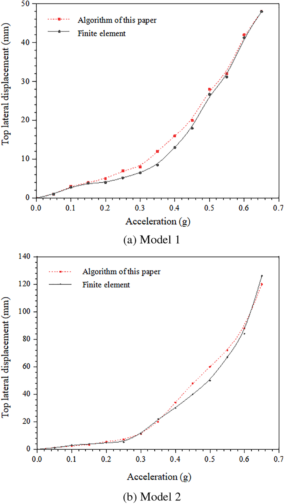
Figure 8: Relation between top displacement and acceleration

Fig. 8 calculates the relationship between the lateral displacement at the top of the panel and the peak acceleration calculated by the constitutive model proposed in this paper, and the displacement calculated by the finite element model. It can be seen from Fig. 8 that the lateral displacement calculated by the stiff-soil constitutive model in this paper is in good agreement with the finite element results. The results show that for model 1 when the acceleration amplitude is less than 0.35 g, the lateral displacement of the panel is small; however, when the acceleration amplitude of the peak acceleration exceeds the threshold acceleration, the lateral displacement of the panel increases more. When the input acceleration amplitude of model 1 of the stiff-soil slip constitutive model is 0.3–0.45 g, the lateral deformation rate will increase substantially. In model 2, the lateral deformation rate increases when the input acceleration amplitude is 0.4–0.55 g, and this large increase in the lateral deformation rate of the wall is also observed in some similar shaking table studies.

In model 1, when the ratio of reinforcement length to reinforcement retaining wall height is 0.6, the lateral deformation rate will increase substantially when the input acceleration amplitude is around 0.35 g. In model 2, when the ratio of reinforcement length to reinforcement retaining wall height is 1, the lateral deformation rate will increase substantially when the input acceleration amplitude is around 0.5 g. This indicates that under the condition of the same spacing of reinforcement, increasing the length of reinforcement can enhance the seismic stability of reinforced earth retaining wall, and the seismic performance of the reinforced earth retaining wall can be enhanced compared with that of a short reinforcement wall, and it can resist the vibration influence of strong seismic acceleration peak. In this example, when the length-height ratio between reinforcement and wall height increases by 33%, the seismic acceleration of reinforced soil retaining wall against large deformation due to lateral displacement increases by 30%, and the seismic performance improves obviously. On the other hand, reinforced soil retaining wall reinforcement is divided into stable zone and unstable zone. When the retaining wall is damaged, the reinforcement in the stable zone does not play a role in the seismic calculation is useless, but the increase of reinforcement length cannot be ignored to improve the seismic performance of the retaining wall, so the design of reinforcement length should be considered reasonably in the seismic design.

Fig. 9 shows the maximum tensile force of reinforcement obtained by three methods. It can be concluded from Fig. 9 that the method in this paper is the maximum tensile value generated by reinforcement in the entire earthquake process. The results show that the maximum reinforcement tension calculated by the AASHTO method and this paper is greater than the maximum reinforcement tension determined by the simplified stiffness method. The tensile value of reinforcement near the bottom of the wall calculated by the AASHTO simplified method is higher than that calculated by the numerical model in this chapter, while the tensile value calculated by the FHWA stiffness method is smaller for all layers except the bottom reinforcement.

Figure 9: Maximum mobilized tension comparison

Fig. 10 shows the tension distribution of reinforcement and the potential fracture surface obtained therefrom. Compared with the classical fracture surface shape, the maximum tension position of reinforcement obtained by this algorithm is consistent with the potential fracture surface. The calculation shows that the tensile force of the reinforced soil retaining wall is not evenly distributed along the length of the reinforced soil retaining wall. The tensile force of the reinforced soil retaining wall at the bottom of the reinforced soil retaining wall is smaller at both ends of the reinforced material and larger in the middle, but the maximum tensile force of the reinforced material appears on the side inclined to the end of the panel. The tension distribution of the upper reinforcement of the retaining wall is the same. The difference is that the maximum value of the tension of the upper reinforcement is biased to the back end.

Figure 10: Reinforcement tension distribution

To observe the change law of displacement, velocity, and acceleration of reinforced earth retaining wall model in the process of earthquake load, some monitoring points are set in the program, and the response of gravity retaining wall in the whole process of an earthquake is analyzed by extracting the monitoring point data. As shown in Fig. 11, the maximum horizontal velocity at the bottom of the retaining wall along the axis is 0.32 m/s in the negative direction and 0.34 m/s in the positive direction. The maximum horizontal velocity occurs at the monitoring point at the top of the wall. The maximum horizontal velocity at the top of the retaining wall along the axis is 1.05 m/s in negative direction and 0.74 m/s in positive direction, which is about 325% and 221% of that at the bottom of the wall. The velocity time-history curve is similar to the curve of seismic waveform. The velocity is smaller in the early phase of vibration, larger in the main phase of vibration, and smaller in the late phase of vibration. As shown in Fig. 12, the maximum negative horizontal displacement at the bottom of the reinforced soil retaining wall model is 0.035 m, the maximum positive horizontal displacement is 0.073 m, the maximum horizontal displacement at the top of the wall is 0.132 m, and the maximum positive horizontal displacement is 0.130 m, about 377% and 178% of the bottom, respectively. The vibration amplitude of the reinforced soil retaining wall is large in the initial vibration phase of the horizontal displacement time history curve. With the increase of time, the vibration amplitude of the horizontal displacement of the retaining wall tends to be stable, and the amplitude of the horizontal displacement decreases. The whole vibration process of the reinforced soil retaining wall maintains a stable state.

Figure 11: Horizontal velocity time history curve

Figure 12: Horizontal displacement time history curve

5  Conclusions

In this paper, a constitutive model of reinforced soil that can consider the mutual sliding between reinforcement and soil is proposed. The finite element dynamic time history calculation program of composite response analysis is compiled by using Fortran language, and the time history analysis of reinforced soil retaining wall and gravity retaining wall is carried out. The main conclusions are as follows:

1.    By comparing the constitutive model of reinforced soil proposed in this paper with previous studies, it can be found that the calculated value of peak strength of the constitutive model is similar to the experimental value. The slip constitutive model of reinforced soil can well simulate the stress-strain behavior of composite materials with no or small slip of reinforcement.

2.    When the peak acceleration is small, the seismic response of the reinforced earth retaining wall is stable. When the acceleration increases beyond a certain threshold, the lateral displacement of the reinforced earth retaining wall panel increases more and the vibration is more severe, which indicates that the reinforced earth retaining wall can maintain good stability under the action of low-intensity earthquake, but will temporarily appear unstable response under the action of a strong earthquake.

3.    Under the condition of the same distance between reinforcement and reinforcement, increasing the length of reinforcement can enhance the seismic stability of reinforced earth retaining wall, and the seismic performance of reinforced earth retaining wall can be enhanced compared with that of shorter reinforcement and can resist the vibration influence of strong seismic acceleration peak. The calculation of the maximum reinforcement tension shows that the maximum reinforcement tension occurs in the bottom area of the reinforced soil retaining wall, and the bottom calculation should be strengthened to prevent damage during the seismic design.

Acknowledgement: Support extended by non-teaching staff and colleagues in conducting physical model tests is appreciated in gratitude.

Funding Statement: This work was supported in part by the Chongqing Social Science Planning Project (2021BS064), Chongqing Construction Science and Technology Plan Project (Grant 2023-0187), Special Foundation of Chongqing Postdoctoral Research (2021XM2052), Scientific and Technological Research Program of Chongqing Municipal Education Commission (Grant KJQN202304703).

Author Contributions: The authors confirm contribution to the paper as follows: study conception and design: Lianhua Ma and Linfeng Han; data collection: Min Huang; analysis and interpretation of results: Lianhua Ma, Min Huang and Linfeng Han; draft manuscript preparation: Lianhua Ma. All authors reviewed the results and approved the final version of the manuscript.

Availability of Data and Materials: The authors confirm that the data supporting the findings of this study are available within the article.

Ethics Approval: Not applicable.

Conflicts of Interest: The authors declare that they have no conflicts of interest to report regarding the present study.

References

1. Steedman RS, Zeng X. The influence of phase on the calculation of pseudo-static earth pressure on a retaining wall. Geotechnique. 1990;40(1):103–12. doi:10.1680/geot.1990.40.1.103. [Google Scholar] [CrossRef]

2. Huang CC. Investigations of soil retaining structures damaged during the Chi-Chi (Taiwan) earthquake. J Chin Inst Eng. 2000;23(4):417–28. doi:10.1080/02533839.2000.9670562. [Google Scholar] [CrossRef]

3. Ling HI, Leshchinsky D, Chou NNS. Post-earthquake investigation on several geosynthetic-reinforced soil retaining walls and slopes during the Ji-Ji earthquake of Taiwan. Soil Dyn Earthq Eng. 2001;21(4):297–313. doi:10.1016/S0267-7261(01)00011-2. [Google Scholar] [CrossRef]

4. Koseki J, Bathurst RJ, Guler E, Kuwano J, Maugeri M. Seismic stability of reinforced soil walls. In: Proceedings of the 8th International Conference on Geosynthetics; 2006; Yokohama, Japan. vol. 1, p. 51–77. [Google Scholar]

5. Garcia-Suarez J, Asimaki D. Exact seismic response of smooth rigid retaining walls resting on stiff soil. Int J Numer Anal Met. 2020;44(13):1750–69. doi:10.1002/nag.3082. [Google Scholar] [CrossRef]

6. Mylonakis G, Kloukinas P, Papantonopoulos C. An alternative to the Mononobe-Okabe equations for seismic earth pressures. Soil Dyn Earthq Eng. 2007;27(10):957–69. doi:10.1016/j.soildyn.2007.01.004. [Google Scholar] [CrossRef]

7. El-Emam MM, Bathurst RJ. Experimental design, instrumentation and interpretation of reinforced soil wall response using a shaking table. Int J Phys Model Geo. 2004;4(4):13–32. [Google Scholar]

8. Vieira CS, de Lurdes Lopes M, Caldeira LM. Earth pressure coefficients for design of geosynthetic reinforced soil structures. Geotext Geomembranes. 2011;5(29):491–501. doi:10.1016/j.geotexmem.2011.04.003. [Google Scholar] [CrossRef]

9. Athanasopoulos-Zekkos A, Vlachakis VS, Athanasopoulos GA. Phasing issues in the seismic response of yielding, gravity-type earth retaining walls–Overview and results from a FEM study. Soil Dyn Earthq Eng. 2013;55(10):59–70. doi:10.1016/j.soildyn.2013.08.004. [Google Scholar] [CrossRef]

10. Tatsuoka F. Seismic stability against high seismic loads of geosynthetic-reinforced soil retaining structures, Keynote Lecture. In: Proceedings of the 6th International Conference on Geosynthetics; 1998; Atlanta, GA, USA. vol. 1, p. 103–42. [Google Scholar]

11. Yang X, Li Z. Kinematical analysis of 3D passive earth pressure with nonlinear yield criterion. Int J Numer Anal Met. 2018;42(7):916–30. doi:10.1002/nag.2771. [Google Scholar] [CrossRef]

12. Fathipour H, Siahmazgi AS, Payan M, Chenari RJ. Evaluation of the lateral earth pressure in unsaturated soils with finite element limit analysis using second-order cone programming. Comput Geotech. 2020;125:103587. doi:10.1016/j.compgeo.2020.103587. [Google Scholar] [CrossRef]

13. Fathipour H, Siahmazgi AS, Payan M, Veiskarami M, Jamshidi Chenari R. Limit analysis of modified pseudodynamic lateral earth pressure in anisotropic frictional medium using finite-element and second-order cone programming. Int J Geomech. 2021a;21(2):04020258. [Google Scholar]

14. Fathipour H, Payan M, Chenari RJ. Limit analysis of lateral earth pressure on geosynthetic-reinforced retaining structures using finite element and second-order cone programming. Comput Geotech. 2021b;134:104119. [Google Scholar]

15. Fathipour H, Payan M, Jamshidi Chenari R, Senetakis K. Lower bound analysis of modified pseudo-dynamic lateral earth pressures for retaining wall-backfill system with depth-varying damping using FEM–Second order cone programming. Int J Numer Anal Met. 2021c;45(16):2371–87. doi:10.1002/nag.3269. [Google Scholar] [CrossRef]

16. Li H, Yang G, Zou Y. Analysis of dynamic characteristics of reinforced soil retaining wall. China J Highway Transport. 2004;17(2):28–31 (In Chinese). [Google Scholar]

17. McGown A, Andrawes KZ, Hasani MM. Effect of inclusion properties on the behavior of sands. Geotechnique. 1978;28(3):327–46. doi:10.1680/geot.1978.28.3.327. [Google Scholar] [CrossRef]

18. Li ZW, Li TZ, Yang XL. Three-dimensional active earth pressure from cohesive backfills with tensile strength cutoff. Int J Numer Anal Met. 2020;44(7):942–61. doi:10.1002/nag.3021. [Google Scholar] [CrossRef]

19. Mirmoazen SM, Lajevardi SH, Mirhosseini SM, Payan M, Jamshidi Chenari R. Limit analysis of lateral earth pressure on geosynthetic-reinforced retaining structures subjected to strip footing loading using finite element and second-order cone programming. IJST-T Civ Eng. 2022;46(4):3181–92. [Google Scholar]

20. Shekarian S, Ghanbari A, Farhadi A. New seismic parameters in the analysis of retaining walls with reinforced backfill. Geotext Geomembranes. 2008;26:350–6. doi:10.1016/j.geotexmem.2008.01.003. [Google Scholar] [CrossRef]

21. Bellezza I. Seismic active soil thrust on walls using a new pseudo-dynamic approach. Geotech Geol Eng. 2015;33(4):795–812. doi:10.1007/s10706-015-9860-1. [Google Scholar] [CrossRef]