
 Submit a Paper
 Propose a Special lssue
 Open Access
ARTICLE

Surface Defect Detection and Evaluation Method of Large Wind Turbine Blades Based on an Improved Deeplabv3+ Deep Learning Model
1 Institution of Earthquake Protection and Disaster Mitigation, Lanzhou University of Technology, Lanzhou, 730050, China
2 International Research Base on Seismic Mitigation and Isolation of GANSU Province, Lanzhou University of Technology, Lanzhou, 730050, China
3 Disaster Prevention and Mitigation Engineering Research Center of Western Civil Engineering, Lanzhou University of Technology, Lanzhou, 730050, China
* Corresponding Author: Wanrun Li. Email:
Structural Durability & Health Monitoring 2024, 18(5), 553-575. https://doi.org/10.32604/sdhm.2024.050751
Received 16 February 2024; Accepted 22 April 2024; Issue published 19 July 2024
 View Full Text
 Download PDF
Abstract
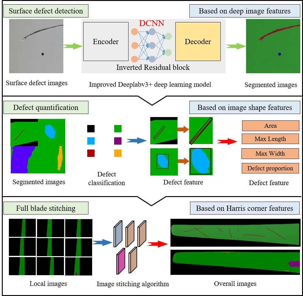
The accumulation of defects on wind turbine blade surfaces can lead to irreversible damage, impacting the aerodynamic performance of the blades. To address the challenge of detecting and quantifying surface defects on wind turbine blades, a blade surface defect detection and quantification method based on an improved Deeplabv3+ deep learning model is proposed. Firstly, an improved method for wind turbine blade surface defect detection, utilizing Mobilenetv2 as the backbone feature extraction network, is proposed based on an original Deeplabv3+ deep learning model to address the issue of limited robustness. Secondly, through integrating the concept of pre-trained weights from transfer learning and implementing a freeze training strategy, significant improvements have been made to enhance both the training speed and model training accuracy of this deep learning model. Finally, based on segmented blade surface defect images, a method for quantifying blade defects is proposed. This method combines image stitching algorithms to achieve overall quantification and risk assessment of the entire blade. Test results show that the improved Deeplabv3+ deep learning model reduces training time by approximately 43.03% compared to the original model, while achieving mAP and MIoU values of 96.87% and 96.93%, respectively. Moreover, it demonstrates robustness in detecting different surface defects on blades across different backgrounds. The application of a blade surface defect quantification method enables the precise quantification of different defects and facilitates the assessment of risk levels associated with defect measurements across the entire blade. This method enables non-contact, long-distance, high-precision detection and quantification of surface defects on the blades, providing a reference for assessing surface defects on wind turbine blades.Graphic Abstract
Keywords
With the rapid increase in the number of wind turbines and the continuous enlargement of wind turbine blade sizes, blade damage has emerged as a critical factor constraining the further development of the wind power generation industry [1,2]. Wind turbine blades, serving as the decisive components of wind power generation systems, suffer significant consequences on wind power efficiency and safe operation when damaged. Common blade damage includes surface Cracks, Spalling, Corrosions, and Holes. These damages have the potential to lead to surface alterations in blade aerodynamic efficiency, subsequently impacting a decrease in power output and the occurrence of safety incidents. This can severely affect the stable operation and economic benefits of wind farms.
To promptly detect damage to wind turbine blades and implement timely maintenance measures, scientifically effective blade damage detection technologies are of paramount importance. The existing damage detection technologies, mainly relying on strain measurement, acoustic emission, ultrasound, thermal imaging, vibration, etc., have been applied in the detection of wind turbines. Blade damage detection based on strain measurements indirectly assesses blade damage through the temperature or strain-induced expansion or contraction of the blades [3]. However, this method requires strain sensors to be installed on the surface of the blade or embedded in the blade layer, which can cause unnecessary damage to the blade and affect its aerodynamic performance [4]. Acoustic emission, ultrasonic, and thermal imaging detections can be conducted through non-contact methods [5–7]. Acoustic emission and ultrasonic testing equipment often find it difficult to detect surface defects on installed wind turbine blades, and operators require a certain level of professional knowledge. Consequently, these methods have not been widely applied in the field of blade surface defect detection. Vibration-based detection methods primarily focus on the identification of abnormal vibrations caused by irregular vibrations and deformations [8]. Vibration-based detection methods require the acquisition of vibration data through sensors such as displacement sensors and acceleration sensors. However, displacement sensors often require a fixed base for measurement while acceleration sensors must be affixed to the blades. The unique structure of the blades is not conducive to sensor installation. Specifically, sensors require extensive cable laying, which leads to significant labor costs. Furthermore, in wind farm environments, the lack of power supply often makes it impractical to use sensors for detecting numerous turbine blades. Despite the maturity of wireless sensor technology being gradually applied in structural health monitoring, the complexities related to data transmission, time synchronization, and power consumption have not been adequately addressed, thus preventing its widespread adoption in blade detection [9].
In recent years, with the continuous development of computer technology and the ongoing updates in hardware, a plethora of computer vision-based structural health monitoring methods have been applied in practical engineering [10–13]. Computer vision utilizes visual sensors to acquire data, achieving non-contact, non-destructive, high-precision, and long-distance structural health monitoring. Therefore, vision-based detection methods are greatly favored by engineers in the field of engineering. Feng et al. [14] employed a template-matching algorithm to conduct vision-based dense full-field displacement measurements on a simply supported beam. Additionally, they performed on-site testing with passing trains on the Manhattan Bridge, thereby validating the real-time capability and multi-point measurement capability of the vision sensors. Jiang et al. [15] developed a vision based lightweight convolutional neural network, combined with drone image acquisition, for detecting and locating bridge cracks, peeling, and corrosion. Johns et al. [16] conducted experimental verification of crane load positioning for curtain wall installation under challenging lighting conditions using a computer vision measurement algorithm without landmark points. Shao et al. [17] proposed an advanced binocular vision system for aimless full-field 3D vibration displacement measurement of civil engineering structures, which is easier to achieve accurate 3D vibration displacement measurement. Visual-based structural health monitoring is an emerging technology that has found applications in diverse fields. This method relies exclusively on cameras or unmanned aerial vehicles for capturing images and obtaining sensor-consistent measurements. Consequently, it presents a more cost-effective alternative to traditional detection methods, which typically entail the use of costly instruments, equipment, and extensive human resources. Thus, integrating computer vision can serve as a valuable complement to conventional approaches.
Vision-based detection methods can effectively facilitate remote and precise monitoring of wind turbines in the operational environment. Numerous researchers have conducted studies on the health monitoring of wind turbine structures using visual methods [18,19]. With the continuous development of deep learning technology and the improvement in hardware computing capabilities, the performance and application scenarios of blade surface defect detection have been significantly enhanced. Although the requirement for a large number of high-resolution images and the considerable time investment for training and image annotation, deep learning can be effectively applied to diverse real-world detection tasks once the surface defect features are determined. Therefore, the time costs associated with training and annotation are deemed acceptable in long-term monitoring tasks, given the benefits derived from the trained model. Yang et al. [20] proposed an image recognition model based on deep learning networks that utilize transfer learning and an ensemble learning classifier based on random forests. This model is employed to automatically extract image features, enabling accurate and efficient detection of damage to wind turbine blades, but it does not involve defect classification. Hacıefendioğlu et al. [21] utilized multiple pre-trained Convolutional Neural Network (CNN) models alongside Score-CAM visualization techniques to characterize icy regions, ice density, and lighting conditions on wind turbine blades. Guo et al. [22] proposed a hierarchical recognition framework for wind turbine blade damage detection and identification, composed of Haar-AdaBoost steps for region proposals and a CNN classifier for damage detection and fault diagnosis on the blade. However, this framework only performs bounding box detection for blade damage and does not achieve high accuracy. Zhu et al. [23] proposed a deep learning-based image recognition model called “Multivariate Information You Only Look Once” (MI-YOLO), which effectively detects surface cracks on wind turbine blades, especially light-colored cracks. However, this model has limitations as it performs bounding box detection without semantic segmentation and is primarily focused on detecting cracks, making it less versatile in detecting other types of defects. Zhang et al. [24] proposed a deep neural network called Mask-MRNet for detecting wind turbine blade faults based on images captured by UAV (unmanned aerial vehicle). Despite the deep neural network of Mask-MRNet employing masks for blade surface defects, there still exist issues regarding low detection accuracy and imprecise mask coverage. While there have been numerous research achievements in visual-based detection of blade surface defects, there still exist challenges related to unclear classification of these defects, limited detection methods, and insufficient monitoring accuracy. Therefore, there is a pressing requirement for an automated, fast, and highly accurate method for blade detection and assessment.
This paper focuses primarily on the issue of detecting and assessing surface defects on large wind turbine blades. The specific sections are as follows: Section 1 provides an overview of the entire study and highlights the limitations within the domain of surface defect detection on wind turbine blades. Section 2 introduces the principles of the Deeplabv3+ deep learning model and proposes an improved method for wind turbine blade surface defect detection based on the Deeplabv3+ deep learning model, incorporating the Mobilenetv2 backbone feature extraction network and transfer learning concepts. In Section 3, surface defect images obtained after detection are utilized for defect quantification. These images are then combined using image stitching principles to provide an overall evaluation of the surface damage condition of the blade. In Section 4, the method proposed in this paper is validated through training. The robustness of the improvement made to the Deeplabv3+ deep learning model is verified by adjusting different models and hyperparameters. Section 5 involves the detection of blade surface defects and the assessment of damage status through practical testing. Section 6 provides a summary of the main conclusions of this study.
2 Improved Deeplabv3+ Deep Learning Model
Most existing methods for blade surface defect detection rely on bounding box methods. However, these methods frequently struggle to accurately and intuitively capture the distinctive characteristics of defects. Semantic segmentation involves taking certain original images as input and transforming them into masks that highlight regions of interest, where each pixel in the image is assigned a category ID based on the object it belongs to. Therefore, semantic segmentation can represent defect characteristics more accurately and intuitively. The precise classification of blade surface defects is essential for swiftly evaluating blade health. Addressing the multi-class semantic segmentation task concerning blade surface defects is an imperative concern that requires attention.
2.1 Deeplabv3+ Deep Learning Model
Deeplabv3+ is a deep learning model proposed by the Google research team, primarily designed for semantic segmentation tasks [25]. Deeplabv3+ performs exceptionally well in semantic segmentation tasks, effectively and accurately segmenting different objects and regions within images. The overall framework of the Deeplabv3+ deep learning model is shown in Fig. 1. Deeplabv3+ comprises two primary components: an Encoder, which performs image feature extraction, and a Decoder, responsible for result prediction. After the original image is fed into the Encoder, it utilizes a DCNN (Deep Convolutional Neural Network) to extract deep-level and shallow-level features. Deep features undergo more down-sampling, resulting in smaller receptive fields, while corresponding shallow features have larger receptive fields. After extracting these two types of features, it is fused in the Decoder. Shallow-level features through feature fusion with deep-level features through a 1 × 1 convolution, followed by four up-sampling operations. Finally, the segmented image is obtained through a 3 × 3 convolution and four additional up-sampling operations. The Deeplabv3+ deep learning model performs a Resize operation on the final obtained semantic segmentation image, ensuring that the resulting image size remains the same as the original image.
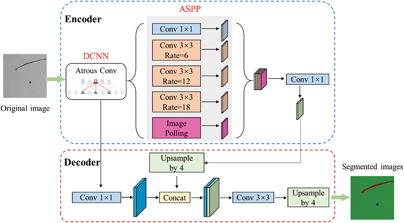
Figure 1: Deeplabv3+ deep learning model network framework
The Deeplabv3+ deep learning model incorporates a significant number of Atrous convolutions in the Encoder section. Atrous convolutions enhance the receptive field without losing information, ensuring that each convolutional output contains a broader range of information. In 2D image signal processing, for each position i on the output feature map y and the convolution filter w, the Eq. (1) for applying Atrous convolution on the input feature map x is as follows:
where
Fig. 2 shows the feature extraction process of an Atrous convolution with a kernel size of 3 × 3, a dilation rate of 2, a stride of 2, and no padding operation. Atrous convolution uses intervals for convolution operations. When the dilation rate is 1, it becomes equivalent to regular convolution. In the convolution operation of Atrous convolution, it is employed to effectively expand the receptive field of output units without increasing the kernel size, which proves particularly advantageous when multiple dilated convolutions are stacked together. For semantic segmentation tasks involving multiple objects and small-sized objects, Atrous convolution can effectively increase the receptive field, thus achieving more precise segmentation results. Hence, the Deeplabv3+ deep learning model, with Atrous convolution as its foundational framework, excels in image segmentation tasks and is regarded as a new pinnacle in semantic segmentation.
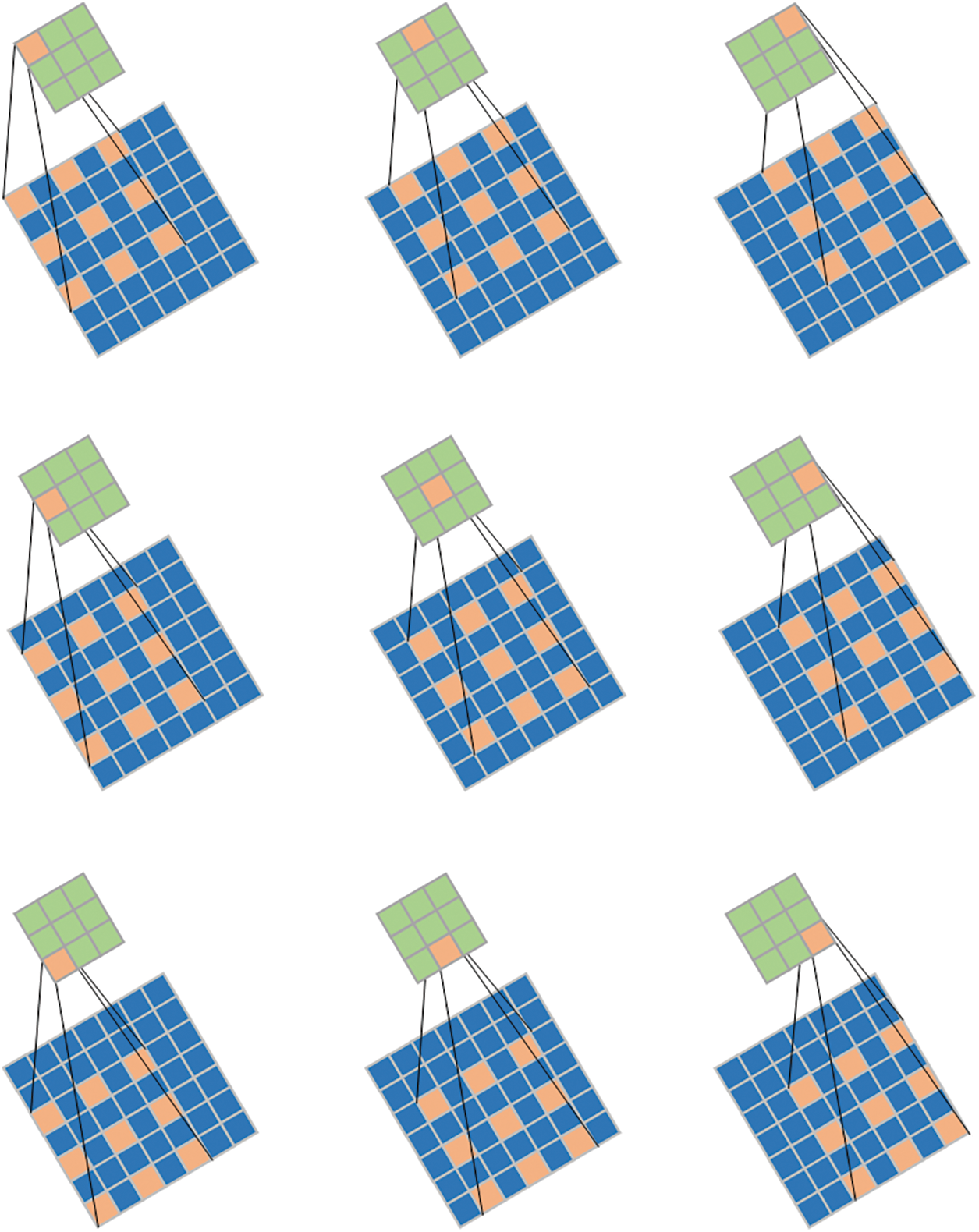
Figure 2: The process of feature extraction using Atrous convolution
The Deeplabv3+ deep learning model employs the ASPP (Atrous Spatial Pyramid Pooling) module in its Encoder to extract deep-level features from images. ASPP enhances the ability of the network to capture multi-scale context without reducing down-sampling, thereby increasing the network’s receptive field. The ASPP module consists of a 1 × 1 regular convolution, three 1 × 1 Atrous convolutions with dilation rates of 6, 12, and 18, and pooling operations. The feature maps are subjected to convolution and pooling operations, followed by feature stacking. After the stacking process, a 1 × 1 regular convolution is applied to generate the output feature map. The ASPP module plays a significant role in the Deeplabv3+ deep learning model and constitutes a vital component of the Deeplabv3+ framework. In this paper, Deeplabv3+ serves as the foundation for constructing a detection model focused on blade surface defects.
2.2 Deeplabv3+ Deep Learning Model
The primary feature extraction in the Deeplabv3+ deep learning model is based on the Xception network. However, the Xception network is relatively complex, and compared to some simpler network architectures, its training may require more time and computational resources [26]. Therefore, to address this concern, this paper adopts the more lightweight Mobilenetv2 network as the feature extraction network for the Deeplabv3+ deep learning model.
Mobilenetv2 is a lightweight deep neural network proposed by the Google team in 2018 [27]. Compared to traditional convolutional neural networks, Mobilenetv2 significantly reduces model parameters and computational complexity while slightly lowering accuracy, making it more suitable for lightweight operations. The Mobilenetv2 network utilizes the Inverted Residual block structure, with the entire Mobilenetv2 architecture being comprised of Inverted Residual blocks. The Inverted Residual block is shown in Fig. 3. The first part starts by utilizing a 1 × 1 convolution for dimension expansion, simultaneously applying BN (Batch Normalization) for normalization, and activating with the ReLU6 function. Subsequently, a 3 × 3 depth-wise separable convolution is employed for feature extraction, succeeded by dimension reduction through a 1 × 1 convolution. The second part serves as the residual shortcut, directly outputting the input feature matrix. The entire Inverted Residual block structure is obtained by adding together the outcomes of the first part and the second part. It is worth noting that for the last 1 × 1 convolution layer in the Inverted Residual block structure, a linear activation function ReLU6 is used instead of the ReLU activation function. The primary rationale behind this choice is that the ReLU activation function tends to induce significant information loss for low-dimensional features, whereas its impact on high-dimensional features is comparatively less pronounced. In the context of the Inverted Residual block structure, the output is a low-dimensional feature vector. Therefore, the use of a linear activation function helps prevent information loss in the features.
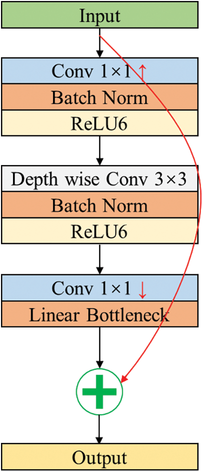
Figure 3: Inverted residual block structure
The Inverted Residual block structure utilizes the ReLU6 function as the activation function, with the ReLU6 function defined by Eq. (2), and its graphical representation is shown in Fig. 4.
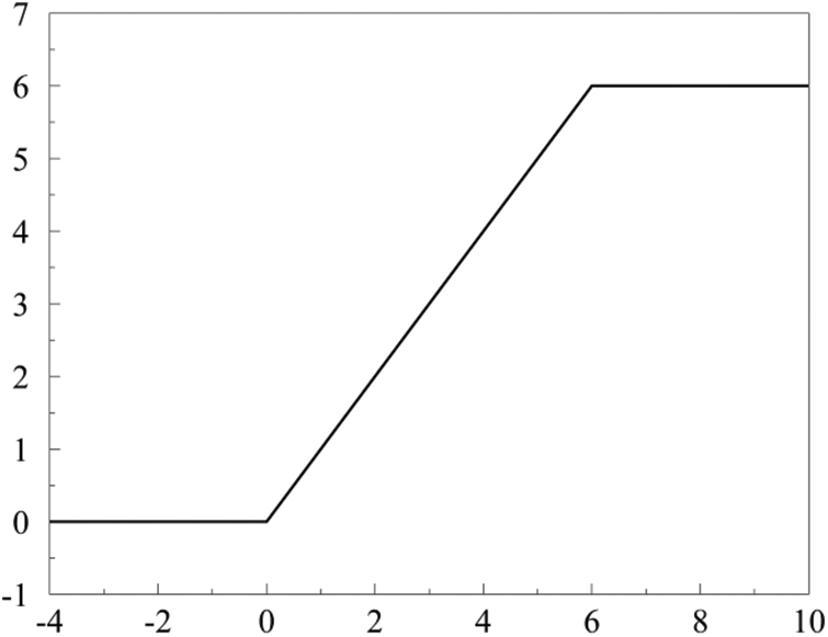
Figure 4: ReLU6 function
ReLU6 is essentially a regular ReLU with the constraint that it limits the maximum output to 6. In the Mobilenetv2 network, its primary purpose is to handle data processing for smaller outputs, allowing for a more precise representation of lightweight task segmentation requirements and to some extent mitigating overfitting issues [28]. Given the nature of the task involved in identifying surface defects on wind turbine blades, which often necessitates a substantial dataset and multiple training iterations, it is crucial to employ ReLU6 as the neural network’s activation function to alleviate the accuracy degradation stemming from excessive training and overfitting due to the extensive dataset.
The model parameters of Mobilenetv2 are shown in Table 1, where t is the expansion factor; c is the depth channel of the output feature matrix; n is the number of repetitions of Bottleneck; s is the stands for stride. After completing the feature extraction of Mobilenetv2, two effective feature layers can be obtained. One effective feature layer is the result of compressing the input image height and width twice, and the other effective feature layer is the result of compressing the input image height and width four times. The two ultimate feature layers are stacked and integrated within the Decoder section. Subsequently, following convolution and up-sampling operations, the segmentation image is obtained.

Transfer learning is an important method in machine learning that aims to transfer knowledge learned from one domain to another. Transfer learning facilitates the migration of pre-existing models or features into another model that requires training, thereby streamlining the learning process for a new task. This method proves especially effective in tasks where data availability is limited. In the field of structural health monitoring, numerous scholars have extensively applied transfer learning in engineering [29,30]. This paper adopts the freeze training strategy in transfer learning to optimize the Deeplabv3+ deep learning model. During the training process, the backbone network is initially frozen in the first half of the epochs, with fine-tuning being performed on only a few layers. During the training process in the latter half of the epochs, the backbone network is unfrozen, and the image features are extracted using the backbone network, with all modules participating in the training. Meanwhile, this paper utilizes pre-trained weights trained by the Google team on the VOC (Visual Object Class) dataset for training on the leaf defect dataset, aiming to expedite model convergence and consequently enhance accuracy. Therefore, the utilization of the freeze training strategy in transfer learning can mitigate the risk of overfitting, and employing the pre-trained weights approach enables rapid model convergence and improved accuracy, facilitating the training of the Deeplabv3+ deep learning model for blade surface defects.
2.4 Improved Deeplabv3+ Deep Learning Model
In this paper, the improved Deeplabv3+ deep learning model is proposed, which utilizes the Deeplabv3+ framework with Mobilenetv2 as the backbone feature extraction network, and integrates a transfer learning freeze training strategy. Table 2 shows the configuration and operation process of the improved Deeplabv3+ deep learning model. The improved Deeplabv3+ deep learning model primarily consists of convolution layers, BN layers, Inverted Residual blocks, ReLU6 and ReLU activation functions, and ASPP. Ultimately, this model generates segmentation images that maintain the same size as the original input image.

In addition to the construction of the overall model, optimizing the deep learning model during the training process to achieve better convergence is of paramount importance. During the transfer learning training process, this paper utilizes the Adam optimization algorithm to optimize the learning rate. This method aims to harness the advantages of both stability and speed, resembling adaptive learning rates. Based on the characteristics of image processing in computer vision, this paper has employed the cosine learning rate decay optimization algorithm to adjust the learning rate during the training of neural networks. This method supports the model to converge more steadily towards the optimal solution. To address the issue of class imbalance, particularly in images with a large number of negative samples and relatively fewer positive samples, this paper utilizes the Focal Loss loss function during training. Training with the Focal Loss loss function can reduce the weight of easily classified samples, consequently enhancing the attention of the model to challenging samples.
The improved Deeplabv3+ deep learning model is composed of both Cross Entropy Loss and Dice Loss as its loss functions. Cross Entropy Loss measures the disparity between the predicted results of the model and the actual results, serving as one of the crucial metrics for optimizing model parameters. In pixel-wise classification during semantic segmentation, a Softmax classifier is employed to balance the Cross Entropy-Loss, using the following Eq. (3):
where
Dice Loss is primarily derived from the Dice coefficient, which is used to assess the similarity between two samples, expressed mathematically as in Eq. (4).
where
In the field of image segmentation, the Dice coefficient can effectively set to zero all pixel values in the predicted segmentation image that do not correspond to the true label. Regarding the activation function, its main purpose is to penalize predictions with low confidence. Therefore, by using the Dice coefficient, a higher level of confidence can be achieved, resulting in a lower Dice Loss, as shown in Eq. (5).
In this paper, the improved Deeplabv3+ deep learning model is proposed for the precise detection of multiple-class surface defects on wind turbine blades. This model is constructed based on the original Deeplabv3+ deep learning architecture, featuring Mobilenetv2 as the backbone feature extraction network, and integrates transfer learning techniques along with training optimization strategies.
3 Evaluation Method for Blade Surface Damage Status
3.1 Quantitative Characteristics of Blade Surface Defects
The main surface defects of wind turbine blades include Cracks, Corrosions, Spalling, and Holes. Most scholars have primarily focused on detecting Cracks in the blades, but they have not conducted multi-target defect recognition [31]. While some scholars have conducted the detection of multiple defects, they have not quantified the defects [32]. Many defects that occur in wind turbine blades during operation can be effectively predicted using quantitative metrics. This enables the anticipation of potential issues under most operating conditions. Furthermore, based on the severity and quantity of defects, maintenance tasks can be scheduled rationally, thereby reducing downtime and maintenance costs. Therefore, the quantification of blade surface defects is of significant importance. To accurately quantify defect data after effective segmentation, this paper utilizes the improved Deeplabv3+ deep learning model for detecting and quantifying different defects based on segmented images, as illustrated in the quantification process shown in Fig. 5. Firstly, precise differentiation of different types of defects is achieved based on the color of the defects. The primary reason for this is that, after using the improved Deeplabv3+ deep learning model for detection, each pixel is classified into different colors according to predefined label categories. Therefore, distinguishing different defects based on colors is feasible. Secondly, different types of defects are assigned specific quantification metrics. For instance, the primary quantification feature for Cracks is Crack width, while for Holes, the primary quantification features are the long diameter and short diameter. Finally, the proportion of different defects is obtained by extracting the overall area of different types of defects.
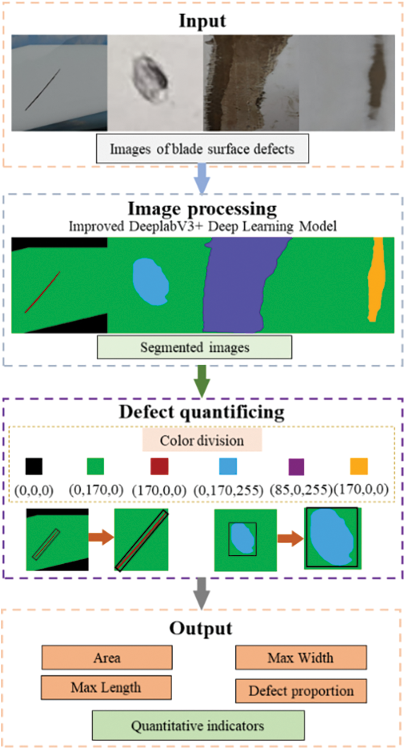
Figure 5: Quantification process for blade surface defects
The presence of Cracks in the blade is primarily measured by Crack width, while Holes are evaluated for their severity in the blade using their respective long and short diameters. As Spalling and Corrosion lack a fixed shape, their measurement is consistently based on the defect area. To attain consistent quantification of all defects, a standardized area calculation is executed, encompassing both the area occupied by surface defects and the areas of the blade and background. Ultimately, blade risk level assessment is conducted based on the overall proportions and quantities of different types of defects. In the calculation of the overall proportions of different types of defects, Eq. (6) is used to calculate the defect area proportions. The defect proportions are normalized to the defect proportion per unit blade.
where
3.2 Evaluation of Overall Blade Surface Defects
Existing wind turbine blades are relatively large, and for the sake of precision, visual-based surface defect detection often utilizes a localized image capture method. When evaluating blade defects, local images cannot provide a more intuitive evaluation of overall blade defects. Therefore, there arises a need for a method involving the stitching of localized images into a global image, facilitating comprehensive assessments of blade defects.
Li et al. proposed an image stitching algorithm based on feature point matching [32]. Due to the reliance on Harris corner feature matching in the image stitching algorithm based on feature point matching, and considering that wind turbine blades often operate in complex backgrounds in practice, previous work involved using pre-processed simple backgrounds for blade image stitching. Once the image stitching process is finalized, challenges may arise in terms of accuracy during detection, primarily stemming from the substantial image size. Additionally, issues related to false positives or false negatives may occur, as the relative defects occupy only a small portion of the image.
To address errors resulting from complex backgrounds during image stitching and enable precise detection of overall blade surface defects, this study adopts a workflow that involves segmenting and detecting images first, followed by image stitching, for the comprehensive assessment of blade surface defects. Firstly, the improved Deeplabv3+ deep learning model is employed to meticulously eliminate the background from blade images. The use of high-resolution images facilitates the precise detection of localized defects on the blade. Subsequently, the segmented images are subjected to an image stitching algorithm based on corner point detection to achieve the overall stitching of blade defect images. It is worth noting that when using segmented images for image stitching, the information contained in the images is simplified since different types of defects, backgrounds, and blades are represented by pre-determined colors in the images. This significantly reduces the computational cost during the image-stitching process and results in a more accurate stitching outcome. Finally, the quantification of blade surface defects is applied to directly measure the different types of defects across the entire blade. This method ultimately accomplishes the objective of assessing the overall blade surface defects.
4.1 Training Environment Facilities and Hyperparameter Settings
To compare the defect detection capabilities of different deep learning models on wind turbine blade surfaces, this study conducted parameter comparisons between the original Deeplabv3+ deep learning model and the improved Deeplabv3+ deep learning model proposed in this paper. The primary hardware and software resources utilized in the training phase of this study are summarized in Table 3, and all models were trained under this specified configuration.

To control the performance and generalization ability of deep learning models, it is necessary to configure the hyperparameters within the network to optimize the training speed and efficiency of the model. In this paper, the categorization will be determined based on whether transfer learning and freeze training techniques are applied. The pre-trained model utilized for transfer learning has undergone pre-training on the VOC dataset, supplying it with pre-trained weights. When employing freeze training, the learning rate is set to 5 × 10⁻⁴ with the Adam optimizer, and it is set to 7 × 10⁻³ with the SGD optimizer. Learning rate decay is performed using two methods: COS and Step. The minimum learning rate for both methods is set to 10% of the original learning rate. All input images have a size of 512 × 512, and the batch size is set to 2.
4.2 Model Evaluation Indicators
To assess the training performance of the deep learning models, this study utilizes accuracy, precision, recall, and MIoU (Mean Intersection over Union) to evaluate the predictive performance of the models.
where TP is the true sample judged to be true; TN is the true sample judged as false; FP is a positive sample that is judged false; FN is a negative sample that is judged as false; m is the number of categories to be predicted.
This paper utilizes a dataset comprising over 3800 images of damaged wind turbine blades, where surface damage primarily encompasses Cracks, Holes, Corrosions, and Spalling, as depicted in Fig. 6. In the training phase, the surface defect dataset is partitioned into a training set and a validation set in a 9:1 ratio, with the validation set employed to evaluate the efficacy of the training process.
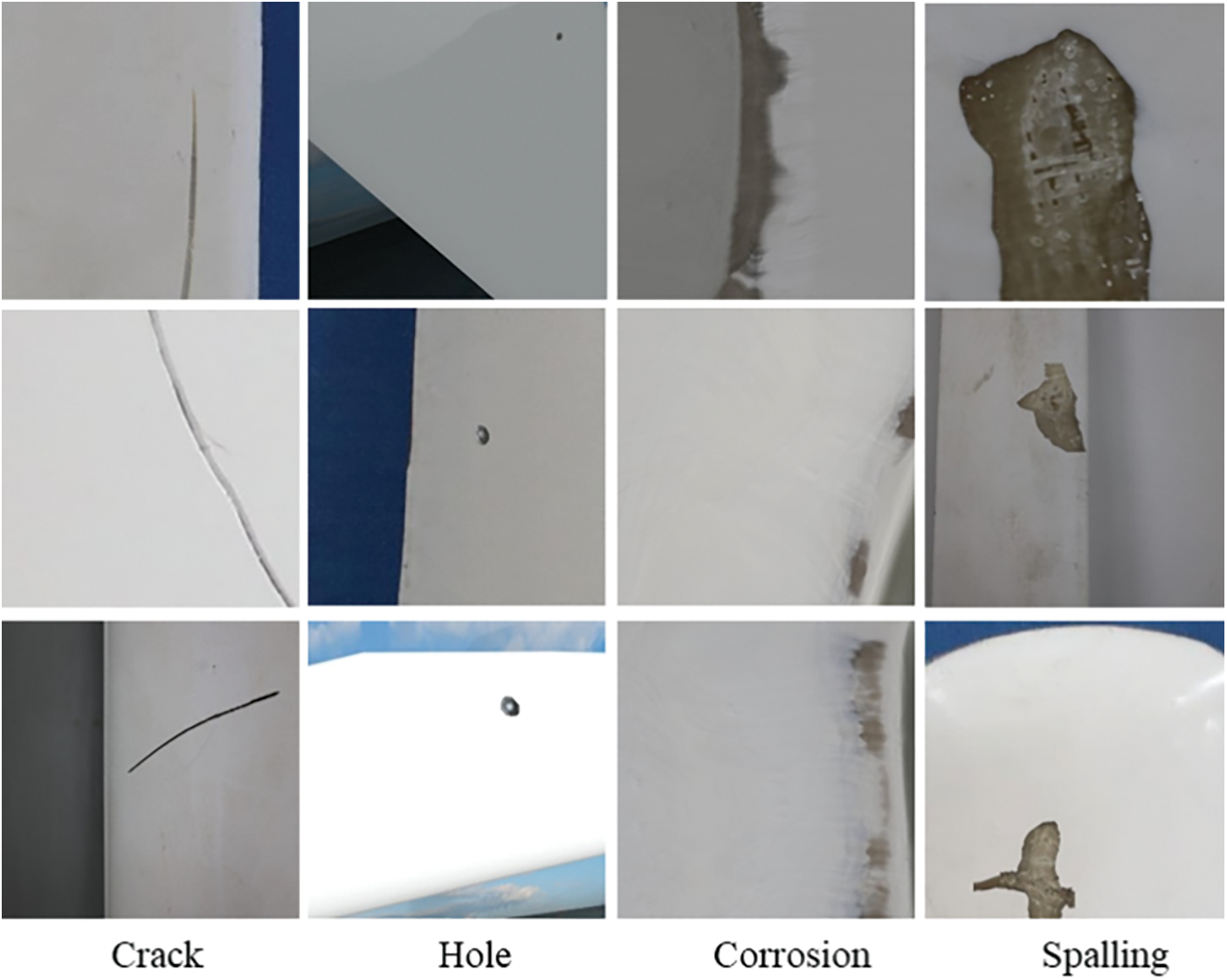
Figure 6: Blade surface defect dataset
The value of the loss function is utilized as a crucial indicator to assess the progress of training, and training is deemed complete when the loss function converges. A smaller converging value indicates better model performance. In this study, different deep learning models will be trained for 400 epochs on this dataset. When employing the transfer learning freeze training strategy, the method entails initially freezing the backbone network for the initial 200 epochs, after which it is unfrozen for the remaining 200 epochs to complete the training process.
4.4 Comparison of Training across Different Models
To effectively compare the detection capabilities of the improved Deeplabv3+ deep learning model proposed in this paper for blade surface defects, the original Deeplabv3+ and the improved Deeplabv3+ deep learning models will be compared under different hyperparameters and modules. The original Deeplabv3+ deep learning model uses Xception as the backbone feature extraction network, while the improved Deeplabv3+ deep learning model uses Mobilenetv2 as the backbone feature extraction network. In 400 epochs, the losses of both using the original training method and using transfer learning for training are shown in Fig. 7.
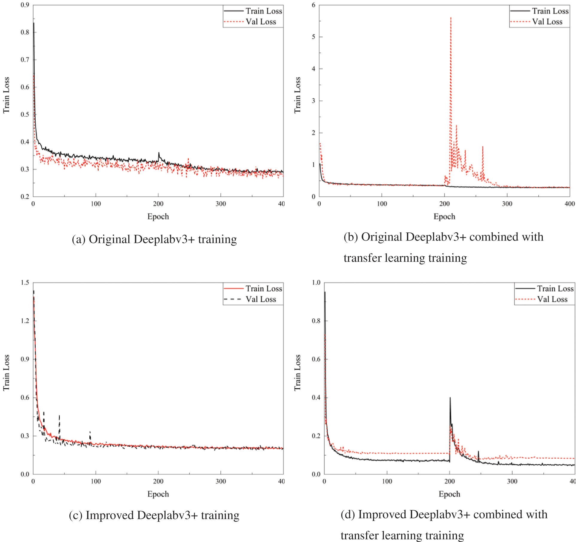
Figure 7: Comparison of different Deeplabv3+ deep learning models under different training conditions
As observed in Figs. 7a and 7c, it is evident that when not employing the transfer learning strategy, the original Deeplabv3+ deep learning model exhibits higher loss values compared to the improved Deeplabv3+ deep learning model. Therefore, the improved Deeplabv3+ deep learning model demonstrates better convergence capabilities. Comparing Figs. 7a and 7b, the application of transfer learning in the original Deeplabv3+ deep learning model does not yield favorable results. After the latter 200 epochs, the validation set experiences significant fluctuations, and the final loss value does not exhibit a significant decrease. Comparing Figs. 7c and 7d, it is evident that although the loss values of the improved Deeplabv3+ deep learning model are already relatively low when using the transfer learning training strategy, there is another decrease in loss values after unfreezing at the 200th epoch, indicating better model convergence. In conclusion, it is evident that the improved Deeplabv3+ deep learning model, when combined with the transfer learning strategy, achieves the best training results and is suitable for blade surface defect segmentation training. To better compare the impact of different parameters on deep learning training and results, Table 4 presents a comparison between the original Deeplabv3+ and the improved Deeplabv3+ deep learning models using different parameters in terms of training duration, accuracy, convergence loss, precision, and recall.

From Table 4, it can be observed that the improved Deeplabv3+ deep learning model, when trained in combination with transfer learning and pre-trained weights, exhibits the best training results. It requires the least amount of training time, and its training loss is significantly lower than the other models. This is primarily attributable to the fact that the improved Deeplabv3+ deep learning model utilizes the lightweight Mobilenetv2 as the backbone feature extraction network. Additionally, the combination of transfer learning and pre-trained weights significantly reduces the training time and enhances the convergence performance of the model. Consequently, the model achieves the highest accuracy, recall rate, and mAP values. Especially when trained using the transfer learning method, the improved Deeplabv3+ deep learning model saves 43.03% of the training time compared to the original Deeplabv3+ deep learning model, significantly enhancing learning efficiency. The original Deeplabv3+ deep learning model, relying on Xception as the backbone feature extraction network, even though it underwent transfer learning and utilizing pre-trained weights, falls short in terms of both training speed and accuracy compared to the improved Deeplabv3+ deep learning model. In summary, based on the training comparison of deep learning models with diverse parameters, the improved Deeplabv3+ deep learning model, incorporating the Adam optimizer and the COS learning rate decay method, exhibits the most outstanding overall performance. Therefore, it can be considered for blade surface defect segmentation training using these parameters.
In semantic segmentation tasks, each pixel in the segmented image is assigned a label category. Therefore, the predicted result and the ground truth are treated as two binary images, with each one representing the segmentation for its respective categories. MIoU (Mean Intersection over Union) assesses the similarity between the predicted results and the ground truth in semantic segmentation tasks by calculating the ratio of the intersection to the union between the two images. It is one of the most important metrics for semantic segmentation tasks. In this paper, a comparison of the MIoU for predicting four defect classes and the MIoU for all classes is presented among the four methods, as shown in Table 5. Due to the verification of the performance of deep learning models with different parameters in Tables 4 and 5 only compares the MIoU calculation results of whether the improved Deeplabv3+ and original Deeplabv3+ deep learning models undergo transfer learning training.

From Table 5, it can be observed that, overall, the MIoU calculation results for different deep learning models are relatively high, especially for the Background and Blade categories, which exhibit the highest values. The improved Deeplabv3+ deep learning model, when combined with transfer learning, achieves a high MIoU of 96.93%, surpassing the other deep learning models. It also significantly outperforms the other deep learning models in the calculation of MIoU for the four defect categories. Therefore, the improved Deeplabv3+ deep learning model, when combined with transfer learning, demonstrates the best training performance and overall effectiveness, making it suitable for predicting surface defects on wind turbine blades.
4.5 Comparison of Model Prediction Results
To provide a concise and intuitive view of the actual prediction performance of different deep learning models, this paper trained the improved Deeplabv3+, original Deeplabv3+, and VGG16Unet (Visual Geometry Group-16 Unet) deep learning models with transfer learning. The predictions of these three classes of deep learning models for different backgrounds, lighting conditions, and defect types are shown in Fig. 8.
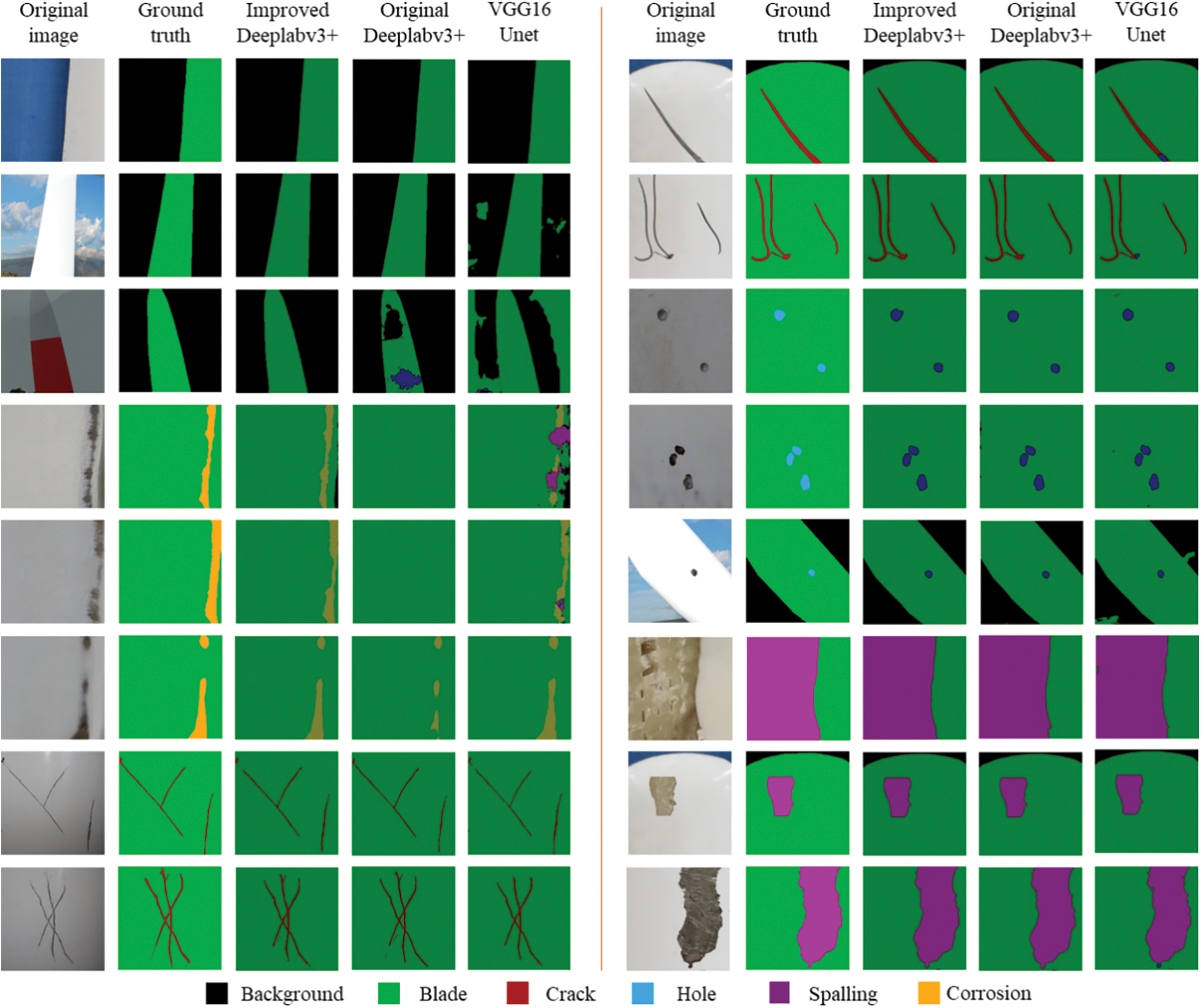
Figure 8: Comparison of blade surface defect segmentation
As shown in Fig. 8, the colors of segmented pixels predicted by different deep learning models do not match the colors of the annotated Ground Truth pixels. The main reason for this inconsistency is the difference generated by the mixing coefficient set during model prediction. However, such issues do not affect the prediction results. From the prediction results, it can be observed that the VGG16Unet deep learning model is sensitive to the background, and it tends to make classification errors in the prediction of different types of defects, leading to mask coverage errors. The original Deeplabv3+ deep learning model performs well overall, but it may encounter segmentation errors or detection failures in cases where the images are blurry or the defect features are not clearly defined. The main reason for this is that when using the Xception backbone feature extraction network, deep-level image features are not fully extracted, leading to inaccurate detection. The improved Deeplabv3+ deep learning model, utilizing Mobilenetv2 as the backbone feature extraction network and employing an inverted residual structure to extract image features, produces segmentation images that closely match the Ground truth images. This model can accurately segment surface defects on wind turbine blades.
In summary, the improved Deeplabv3+ deep learning model, when integrated with the transfer learning strategy, demonstrates both a substantial enhancement in training speed and high precision in model performance metrics such as accuracy, recall, mAP, and MIoU. Concerning its prediction capability, the model can accurately classify and mask surface defects on wind turbine blades, showcasing strong performance in all aspects of surface defect detection on these blades. Therefore, in practical predictions, this study will use the improved Deeplabv3+ deep learning model combined with transfer learning strategies for the detection of surface defects on wind turbine blades.
5 Evaluation of Actual Blade Surface Defect Status
5.1 Measurement of Blade Surface Defects
To accurately quantify surface defects on the blades, this study will utilize the method outlined in Section 3.1 to quantify the four types of surface defects on the blades effectively. The blade surface defects are represented using images with a resolution of 512 × 512 pixels, and the defect segmentation is illustrated in Fig. 9. The specific quantitative metrics are provided in Table 6. To standardize the quantification of blade surface defects, Table 6 employs area, major axis, minor axis, and defect ratio as quantitative criteria for all defects. For Holes, the major and minor axes are measured as the major and minor axes of the circumscribed ellipse, while for other defects, it is determined as the maximum length and maximum width.
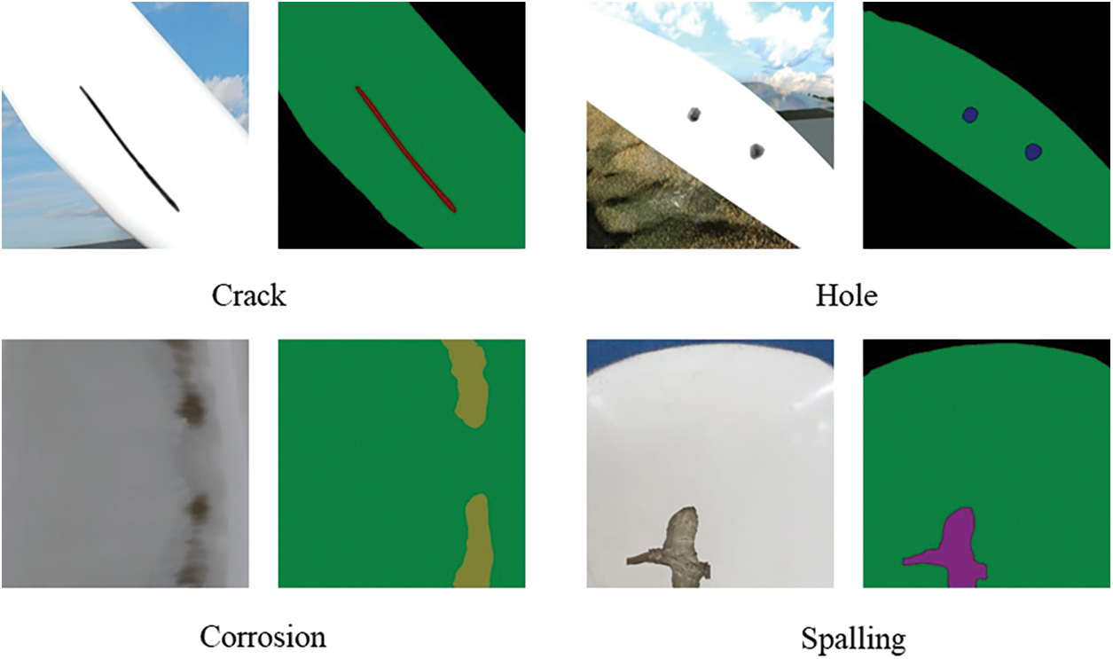
Figure 9: Segmentation of different surface defects on the blade
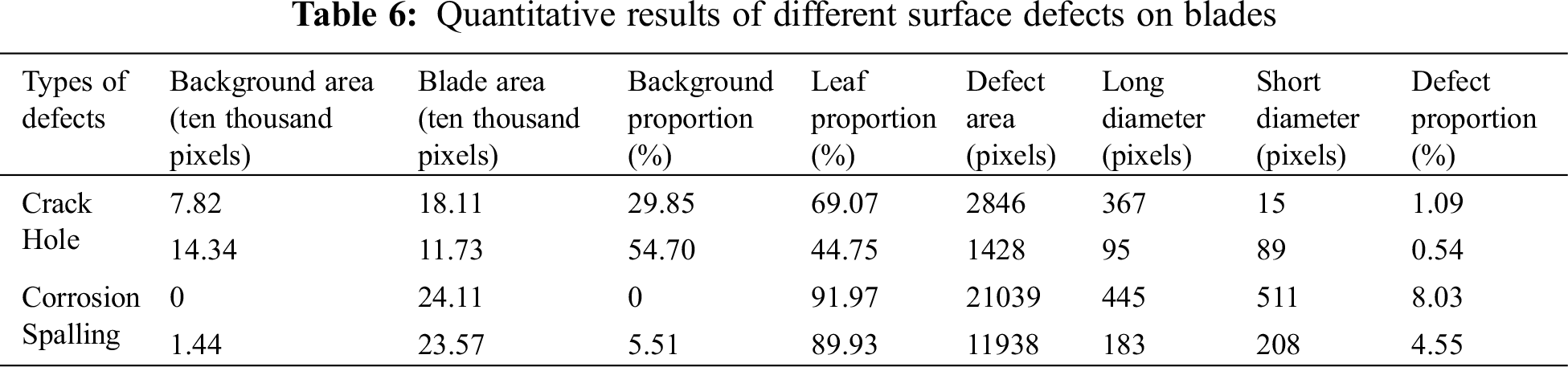
As shown in Fig. 9 and Table 6, while accurately identifying the four types of surface defects, the quantification is refined by considering the areas of the background, blade, and the four defect categories in proportion to the total defect area. Based on the surface defect statistics presented in Table 6, it becomes apparent that distinct defects display varying characteristics. To achieve a more precise quantification of overall defects, this study employs a normalized quantification approach. Specifically, Crack is quantified using the maximum width, Hole is quantified using the major axis length, and Corrosion and Spalling are quantified using the area. This normalization results in the proportions of each defect type and the total defect proportion. The standards for quantification and assessment of visual surface defect detection in this paper primarily draw reference from the quantification parameters used in post-earthquake bridge assessments [33]. Regarding the assessment of surface defects on the blades, the damages are categorized into three classes: low risk, medium risk, and high risk. The classification is based on the number of defects and the total percentage of defects. The differences in image capture methods and the proportion of background in different scenarios lead to variations in the evaluation criteria. Therefore, the primary focus lies on the quantity of defects and the proportion of defects in the assessment.
Fig. 10 shows six segmented images of the four categories of surface defects on blades under different backgrounds, and Table 7 lists the quantitative indicators of different surface defects, ultimately obtaining the overall damage indicators. To holistically assess surface defects on blades, defects occupying less than 10% of the blade are classified as risk level I, those occupying 10% to 30% are categorized as risk level II, and those occupying more than 30% fall into category III. Combining Fig. 10 with Table 7 provides a visual means of assessing defect damage on individual blade photos. It accurately identifies the proportions of the four types of defects under different backgrounds. Ultimately, the risk level of damage is ascertained based on the proportion of defects within the blade. Therefore, using the defect damage assessment method described in Section 3.1 of this paper can accurately identify defects in complex backgrounds and assess the risk level of blades based on the proportion of surface defects.
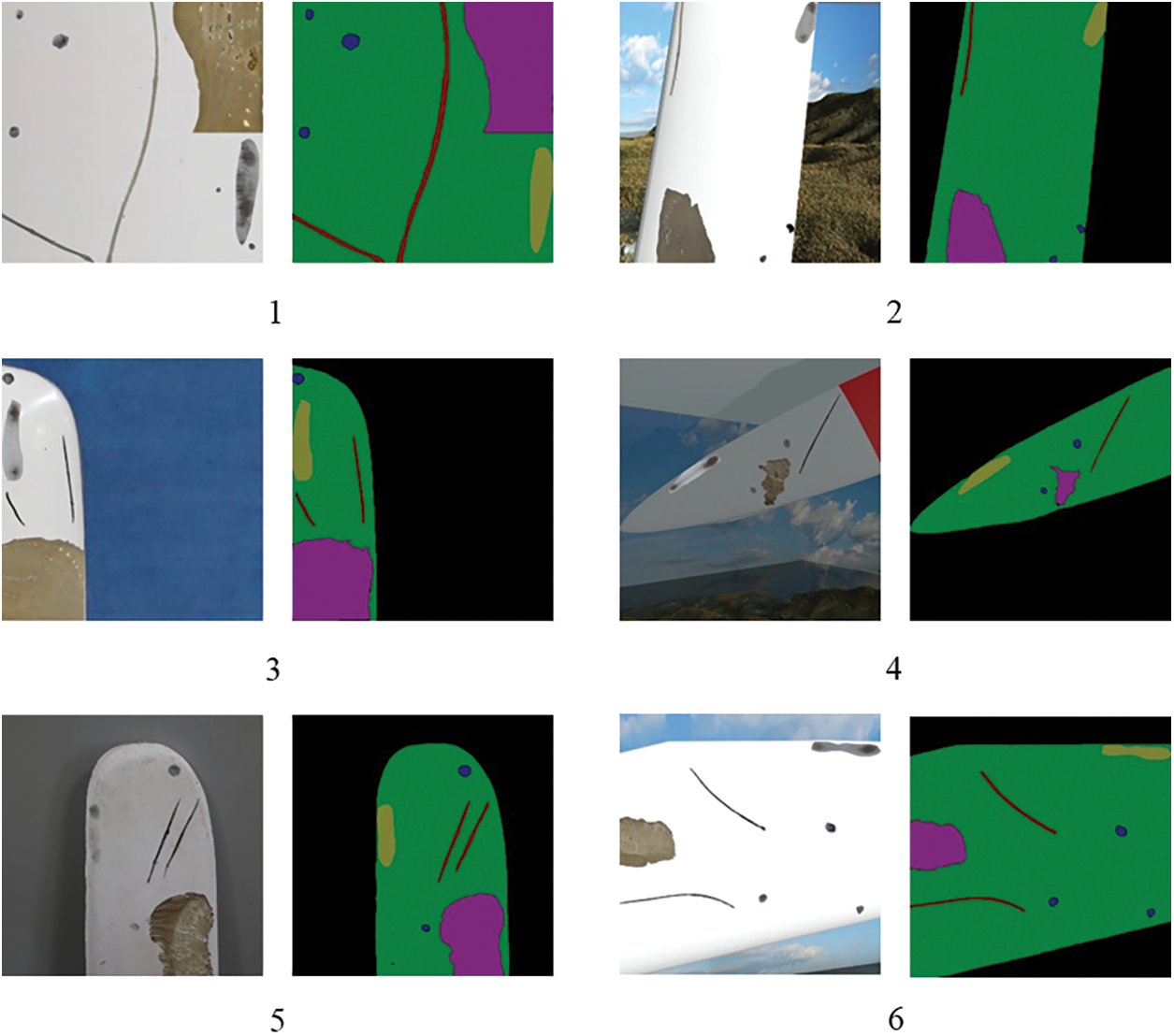
Figure 10: Evaluation image of blade surface defects

5.2 Measurement of Surface Defects on Integral Blades
When capturing images using a camera or UAV, it is often not possible to capture the entire blade in a single shot. Therefore, image stitching is commonly employed to create a complete blade image. However, conducting defect detection on the stitched image after image stitching can lead to significant issues of missed defect detection due to the small proportion of defects in the stitched image. Therefore, in this study, defect detection is initially conducted using local images, which is then followed by an image stitching algorithm. This method effectively avoids the issue of missed defect detection that can occur when stitching original images together and enhances the accuracy of surface defect detection on the blade. Fig. 11 shows the defect detection process on both sides of a blade. It commences with capturing local images of the blade using five separate images. Subsequently, the improved Deeplabv3+ deep learning model is utilized for surface defect detection. Finally, an image stitching procedure is performed to display the surface defects across the entire blade.
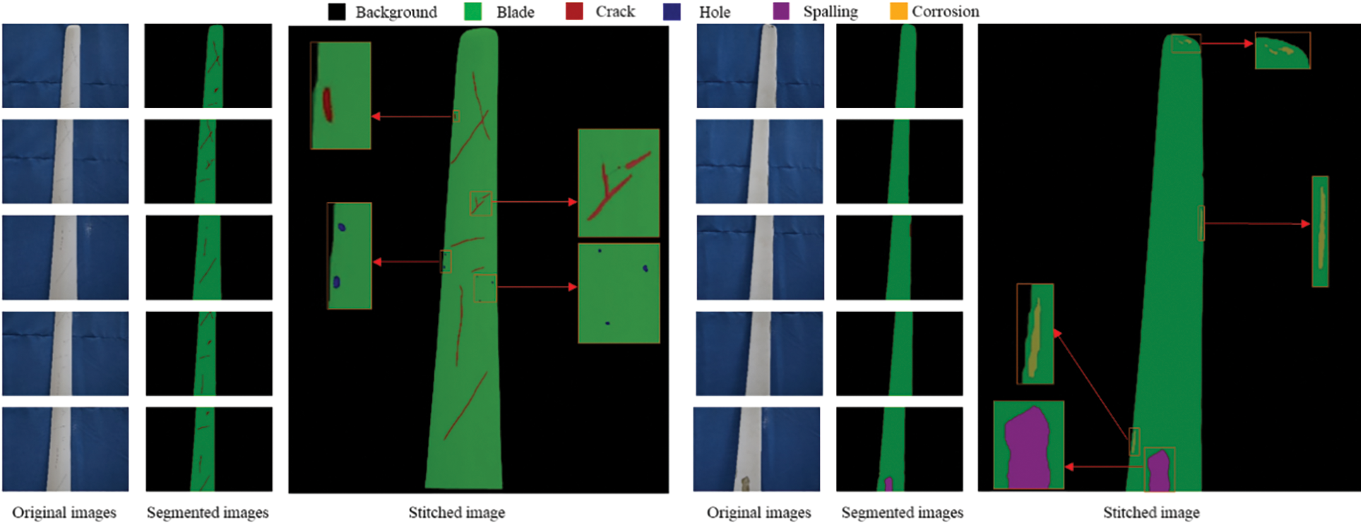
Figure 11: Surface defect detection of integral blades
Fig. 11 demonstrates that utilizing a detect-then-stitch approach enables a more thorough surface defect detection. Additionally, due to background removal, the image stitching process is significantly less time-consuming. According to the defect assessment method for the front side of the blade in Fig. 11, it is determined that defects occupy 2.03% of the blade. However, due to the presence of multiple cracks, the risk level is assessed as level II. On the backside of the blade, it is observed that defects occupy 3.56% of the blade area, and since there are fewer defects, the risk level is assessed as level I.
Based on the improved Deeplabv3+ deep learning model and the surface defect assessment method, effective detection and evaluation of surface defects on wind turbine blades can be performed. When combined with image stitching algorithms, this method enables a comprehensive assessment of surface defects across the entire blade.
This paper proposes an improved Deeplabv3+ deep learning model-based method for the comprehensive detection and assessment of surface defects on wind turbine blades, addressing the challenge of incomplete defect detection on the blade surfaces. Firstly, a framework for detecting surface defects on the wind turbine blades is established. This is achieved by replacing the backbone feature extraction network of the original Deeplabv3+ model with the Mobilenetv2 backbone feature extraction network, resulting in an improved Deeplabv3+ deep learning model tailored for blade surface defect detection. Secondly, by incorporating pre-trained weights through transfer learning and implementing a frozen learning strategy, the training process is further optimized, leading to improved training speed and model convergence accuracy. Finally, a comprehensive detection of surface defects on the blades and an assessment of damage risk levels are performed using surface defect quantification methods and risk evaluation techniques. Based on the research, the following conclusions can be drawn:
(1) The improved Deeplabv3+ deep learning model, employing Mobilenetv2 as the backbone feature extraction network and incorporating transfer learning techniques, can effectively and accurately detect blade surface defects in different environmental conditions.
(2) During the training of the enhanced Deeplabv3+ deep learning model for surface defect detection, a reduction in training time of approximately 43.03% was achieved, while maintaining the mAP of 96.87% and the MIoU of 96.93%. This significantly enhances both the learning efficiency and model accuracy.
(3) Utilizing the defect segmentation images generated by the improved Deeplabv3+ deep learning model, surface defect measurements are conducted. This method using unit blades as a reference, provides a more effective means for assessing the risk associated with surface defects on the wind turbine blades.
(4) The method of segmenting and then reassembling the entire blade effectively addresses the limitation of accurate detection for small defects, resulting in a more precise overall assessment of blade surface defects.
Acknowledgement: Thanks to all team members for their work and contributions.
Funding Statement: The authors disclosed receipt of the following financial support for the research, authorship, and/or publication of this article: This study is supported by the National Science Foundation of China (Grant Nos. 52068049 and 51908266), the Science Fund for Distinguished Young Scholars of Gansu Province (No. 21JR7RA267), and Hongliu Outstanding Young Talents Program of Lanzhou University of Technology.
Author Contributions: The authors confirm contribution to the paper as follows: study conception and design: Wanrun Li, Wenhai Zhao; data collection: Wenhai Zhao; analysis and interpretation of results: Wenhai Zhao, Wanrun Li, Tongtong Wang, Yongfeng Du; draft manuscript preparation: Wenhai Zhao, Wanrun Li, Tongtong Wang, Yongfeng Du. All authors reviewed the results and approved the final version of the manuscript.
Availability of Data and Materials: The data used to support the findings of the study are available from the corresponding author upon request.
Conflicts of Interest: The authors declare that they have no conflicts of interest to report regarding the present study.
References
1. Asghar AB, Liu X. Adaptive neuro-fuzzy algorithm to estimate effective wind speed and optimal rotor speed for variable-speed wind turbine. Neurocomputing. 2018;272:495–504. doi:10.1016/j.neucom.2017.07.022. [Google Scholar] [CrossRef]
2. Joshuva A, Sugumaran V. Comparative study on tree classifiers for application to condition monitoring of wind turbine blade through histogram features using vibration signals: a data-mining approach. Struct Durability Health Monit. 2019;13(4):399–416. doi:10.32604/sdhm.2019.03014. [Google Scholar] [CrossRef]
3. Ozbek M, Rixen DJ. Operational modal analysis of a 2.5 MW wind turbine using optical measurement techniques and strain gauges. Wind Energy. 2013;16(3):367–81. doi:10.1002/we.v16.3. [Google Scholar] [CrossRef]
4. Qiao W, Lu D. A survey on wind turbine condition monitoring and fault diagnosis—part I: components and subsystems. IEEE Trans Ind Electron. 2015;62(10):6536–45. doi:10.1109/TIE.2015.2422112. [Google Scholar] [CrossRef]
5. Nair A, Cai CS. Acoustic emission monitoring of bridges: review and case studies. Eng Struct. 2010;32(6):1704–14. doi:10.1016/j.engstruct.2010.02.020. [Google Scholar] [CrossRef]
6. Amenabar I, Mendikute A, López-Arraiza A, Lizaranzu M, Aurrekoetxea J. Comparison and analysis of non-destructive testing techniques suitable for delamination inspection in wind turbine blades. Compos Part B. 2011;42(5):1298–305. doi:10.1016/j.compositesb.2011.01.025. [Google Scholar] [CrossRef]
7. Muñoz CQG, Márquez FPG, Tomás JMS. Ice detection using thermal infrared radiometry on wind turbine blades. Measurement. 2016;93:157–63. doi:10.1016/j.measurement.2016.06.064. [Google Scholar] [CrossRef]
8. Yan YJ, Cheng L, Wu ZY, Yam LH. Development in vibration-based structural damage detection technique. Mech Syst Signal Process. 2007;21(5):2198–211. doi:10.1016/j.ymssp.2006.10.002. [Google Scholar] [CrossRef]
9. Qiao W, Lu D. A survey on wind turbine condition monitoring and fault diagnosis—part II: signals and signal processing methods. IEEE Trans Ind Electron. 2015;62(10):6546–57. doi:10.1109/TIE.2015.2422394. [Google Scholar] [CrossRef]
10. Felipe-Sesé L, Díaz FA. Damage methodology approach on a composite panel based on a combination of Fringe Projection and 2D Digital Image Correlation. Mech Syst Signal Process. 2018;101:467–79. doi:10.1016/j.ymssp.2017.09.002. [Google Scholar] [CrossRef]
11. Spencer Jr BF, Hoskere V, Narazaki Y. Advances in computer vision-based civil infrastructure inspection and monitoring. Engineer. 2019;5(2):199–222. doi:10.1016/j.eng.2018.11.030. [Google Scholar] [CrossRef]
12. Zhou Y, Ji A, Zhang L. Sewer defect detection from 3D point clouds using a transformer-based deep learning model. Automat Constr. 2022;136:104163. doi:10.1016/j.autcon.2022.104163. [Google Scholar] [CrossRef]
13. Eşlik AH, Akarslan E, Hocaoğlu FO. Short-term solar radiation forecasting with a novel image processing-based deep learning approach. Renew Energy. 2022;200:1490–505. doi:10.1016/j.renene.2022.10.063. [Google Scholar] [CrossRef]
14. Feng D, Feng MQ. Experimental validation of cost-effective vision-based structural health monitoring. Mech Syst Signal Process. 2017;88:199–211. doi:10.1016/j.ymssp.2016.11.021. [Google Scholar] [CrossRef]
15. Jiang S, Cheng Y, Zhang J. Vision-guided unmanned aerial system for rapid multiple-type damage detection and localization. Struct Health Monit. 2023;21(1):319–37. doi:10.1177/14759217221084878. [Google Scholar] [CrossRef]
16. Johns B, Abdi E, Arashpour M. Crane payload localisation for curtain wall installation: a markerless computer vision approach. Measurement. 2023;221:113459. doi:10.1016/j.measurement.2023.113459. [Google Scholar] [CrossRef]
17. Shao Y, Li L, Li J, An S, Hao H. Computer vision based target-free 3D vibration displacement measurement of structures. Eng Struct. 2021;246:113040. doi:10.1016/j.engstruct.2021.113040. [Google Scholar] [CrossRef]
18. Joshuva A, Sugumaran V. Crack detection and localization on wind turbine blade using machine learning algorithms: a data mining approach. Struct Durability Health Monit. 2019;13(2):181–203. doi:10.32604/sdhm.2019.00287. [Google Scholar] [CrossRef]
19. Khadka A, Fick B, Afshar A, Tavakoli M, Baqersad J. Non-contact vibration monitoring of rotating wind turbines using a semi-autonomous UAV. Mech Syst Signal Process. 2020;138:106446. doi:10.1016/j.ymssp.2019.106446. [Google Scholar] [CrossRef]
20. Yang X, Zhang Y, Lv W, Wang D. Image recognition of wind turbine blade damage based on a deep learning model with transfer learning and an ensemble learning classifier. Renew Energy. 2021;163:386–97. doi:10.1016/j.renene.2020.08.125. [Google Scholar] [CrossRef]
21. Hacıefendioğlu K, Başağa HB, Yavuz Z, Karimi MT. Intelligent ice detection on wind turbine blades using semantic segmentation and class activation map approaches based on deep learning method. Renew Energy. 2022;182:1–16. doi:10.1016/j.renene.2021.10.025. [Google Scholar] [CrossRef]
22. Guo J, Liu C, Cao J, Jiang D. Damage identification of wind turbine blades with deep convolutional neural networks. Renew Energy. 2021;174:122–33. doi:10.1016/j.renene.2021.04.040. [Google Scholar] [CrossRef]
23. Zhu X, Hang X, Gao X, Yang X, Xu Z, Wang Y, et al. Research on crack detection method of wind turbine blade based on a deep learning method. Appl Energ. 2022;328:120241. doi:10.1016/j.apenergy.2022.120241. [Google Scholar] [CrossRef]
24. Zhang C, Wen C, Liu J. Mask-MRNet: a deep neural network for wind turbine blade fault detection. J Renew Sustain Energy. 2020;12(5):053302. doi:10.1063/5.0014223. [Google Scholar] [CrossRef]
25. Chen LC, Zhu Y, Papandreou G, Schroff F, Adam H. Encoder-decoder with atrous separable convolution for semantic image segmentation. In: Proceedings of the European Conference on Computer Vision (ECCV); 2018 Sep 8–14; Munich, Germany. [Google Scholar]
26. Chollet F. Xception: Deep learning with depthwise separable convolutions. In: Proceedings of the IEEE Conference on Computer Vision and Pattern Recognition (CVPR); 2017 Jul 21–26; Honolulu, Hawaii, USA. [Google Scholar]
27. Sandler M, Howard A, Zhu M, Zhmoginov A, Chen LC. Mobilenetv2: Inverted residuals and linear bottlenecks. In: Proceedings of the IEEE Conf Comput Vis Pattern Recog (CVPR); 2018 Jun 18–22; Salt Lake City, USA. [Google Scholar]
28. Kim H, Park J, Lee C, Kim JJ. Improving accuracy of binary neural networks using unbalanced activation distribution. In: Proceedings of the IEEE/CVF Conference on Computer Vision and Pattern Recognition (CVPR); 2021 Jun 10–25; Nashville, TN, USA. [Google Scholar]
29. Chen SX, Zhou L, Ni YQ, Liu XZ. An acoustic-homologous transfer learning approach for acoustic emission-based rail condition evaluation. Struct Health Monit. 2021;20(4):2161–81. doi:10.1177/1475921720976941. [Google Scholar] [CrossRef]
30. Jamil F, Verstraeten T, Nowé A, Peeters C, Helsen J. A deep boosted transfer learning method for wind turbine gearbox fault detection. Renew Energy. 2022;197:331–41. doi:10.1016/j.renene.2022.07.117. [Google Scholar] [CrossRef]
31. Wang L, Zhang Z, Luo X. A two-stage data-driven approach for image-based wind turbine blade crack inspections. IEEE ASME Trans Mechatron. 2019;24(3):1271–81. doi:10.1109/TMECH.3516. [Google Scholar] [CrossRef]
32. Li W, Pan Z, Hong N, Du Y. Defect detection of large wind turbine blades based on image stitching and improved UNet network. J Renewe Sustain Energy. 2023;15(1):013302. doi:10.1063/5.0125563. [Google Scholar] [CrossRef]
33. Ye XW, Ma SY, Liu ZX, Ding Y, Li ZX, Jin T. Post-earthquake damage recognition and condition assessment of bridges using UAV integrated with deep learning approach. Struct Control Health Monit. 2022;29(12):e3128. [Google Scholar]
Cite This Article
 Copyright © 2024 The Author(s). Published by Tech Science Press.
This work is licensed under a Creative Commons Attribution 4.0 International License , which permits unrestricted use, distribution, and reproduction in any medium, provided the original work is properly cited.
 Downloads
 Citation Tools