
 Submit a Paper
 Propose a Special lssue
 Open Access
ARTICLE

Bearing Fault Diagnosis Based on Optimized Feature Mode Decomposition and Improved Deep Belief Network
School of Mechanical Engineering, Hebei University of Science and Technology, Shijiazhuang, 050018, China
* Corresponding Author: Guangfei Jia. Email:
(This article belongs to the Special Issue: Sensing Data Based Structural Health Monitoring in Engineering)
Structural Durability & Health Monitoring 2024, 18(4), 445-463. https://doi.org/10.32604/sdhm.2024.049298
Received 02 January 2024; Accepted 01 March 2024; Issue published 05 June 2024
 View Full Text
 Download PDF
Abstract
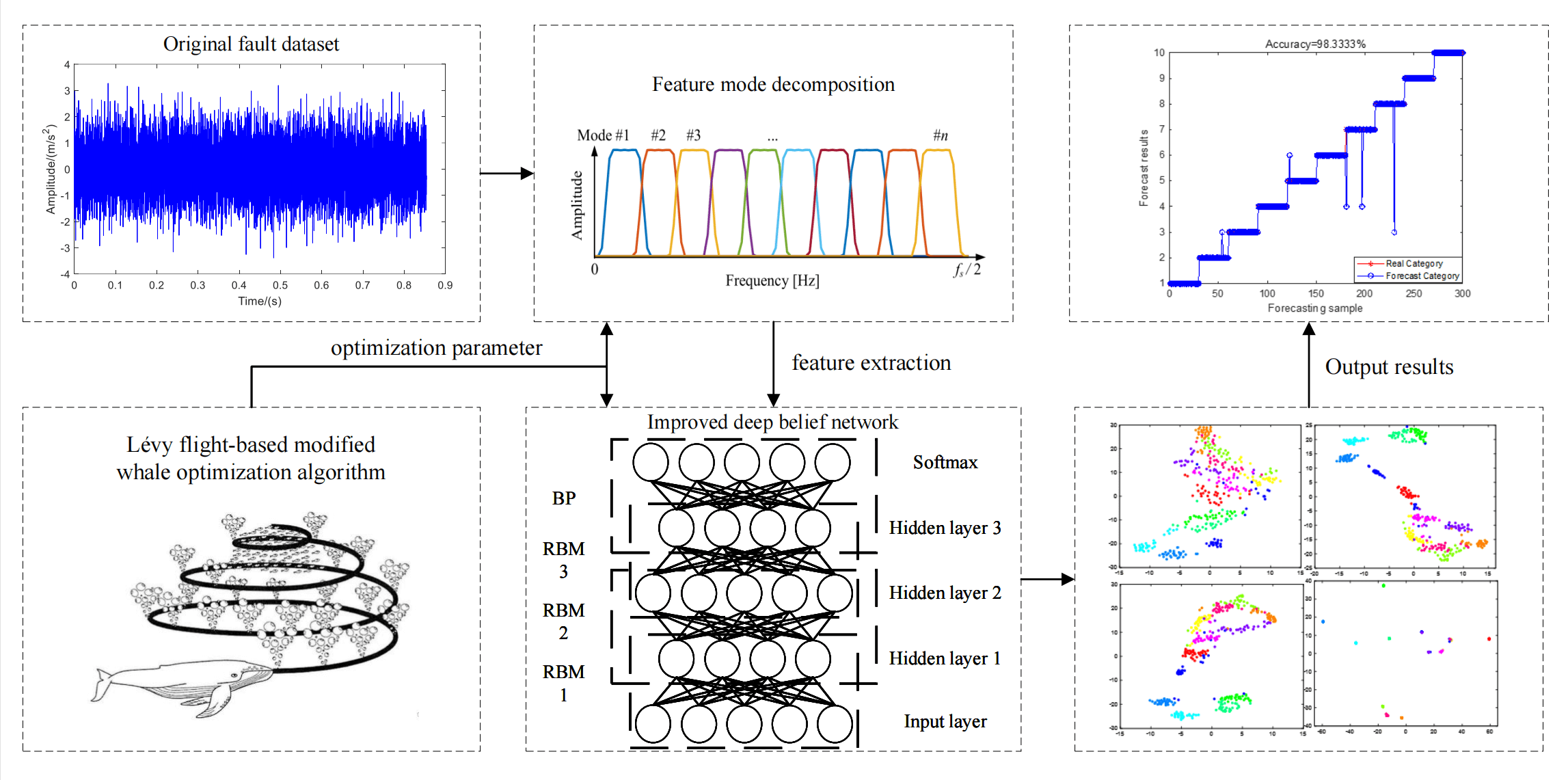
The vibration signals of rolling bearings exhibit nonlinear and non-stationary characteristics under the influence of noise. In intelligent fault diagnosis, unprocessed signals will lead to weak fault characteristics and low diagnostic accuracy. To solve the above problem, a fault diagnosis method based on parameter optimization feature mode decomposition and improved deep belief networks is proposed. The feature mode decomposition is used to decompose the vibration signals. The parameter adaptation of feature mode decomposition is implemented by improved whale optimization algorithm including Levy flight strategy and adaptive weight. The selection of activation function and parameters is crucial in the application of deep belief networks. The improved deep belief networks are proposed based on Hard swish activation function and the improved whale optimization algorithm. The optimized diagnosis model is applied to weak fault diagnosis of bearings. The experimental results show that this method has faster convergence speed and anti-noise performance under the interference of −5 db noise, and effectively improves the adaptive feature extraction ability of the model and the accuracy of fault diagnosis. Under different conditions, the average accuracy reached 97.8% and 97.6%, with good generalization performance.Graphic Abstract
Keywords
Nomenclature
| CEEMD | Complementary ensemble empirical mode decomposition |
| CWRU | Case Western Reserve University |
| DBN | Deep belief network |
| EMD | Empirical mode decomposition |
| EEMD | Ensemble empirical mode decomposition |
| FFR | Fault feature ratio |
| FIR | Finite-impulse response |
| FMD | Feature mode decomposition |
| GWO | Grey wolf optimization |
| IDBN | Improved deep belief network |
| IMF | Intrinsic mode functions |
| LMWOA | Lévy flight-based modified whale optimization algorithm |
| PSO | Particle swarm optimization |
| RBM | Restricted Boltzmann machine |
| SVM | Support vector machine |
| VMD | Variational mode decomposition |
| WOA | Whale optimization algorithm |
Bearing plays an indispensable role in the field of industry and manufacturing, which is an important part of industrial machinery [1–3]. Bearings are prone to malfunctions during operation when bearing various dynamic loads, which directly affects the performance and running state of the entire mechanical system [4,5]. Therefore, it is of great significance to extract bearing fault feature information and carry out fault diagnosis in time.
The fault diagnosis process generally comprises: data collection, feature extraction, feature fusion, and fault recognition. Among these steps, feature extraction is the most crucial because it directly impacts the accuracy of fault diagnosis. However, the vibration signal mixed with noise exhibits a nonlinear and nonstationary state. The fault features are difficult to derive directly from it. EMD can adaptively decompose the signal into several intrinsic mode components [6]. It separates components containing fault features from complex signals. However, its application in the field of fault diagnosis has some defects due to mode mixing and boundary effect [7,8]. EEMD and CEEMD add white noise based on EMD to reduce modal aliasing [9,10]. They enhance the decomposition ability and reduce the phenomenon of mode mixing. However, there is a lot of residual noise in the reconstructed signal, which cannot effectively solve the problem of the endpoint effect. Dragomiretskiy et al. [11] proposed the VMD, which can decompose the signal into multiple narrowband signals with different frequencies [12]. Due to the choice of filter shape and bandwidth, its decomposition ability is closely related to these parameters. This will result in the loss of many additional redundant modes or some important details. Miao et al. [13] proposed FMD decomposition using adaptive FIR filter banks and maximum correlation kurtosis deconvolution theory to solve this problem. FMD has good noise resistance, which can also consider the impulsivity and periodicity of the signal. Because FMD needs preset parameter values, the parameter values affect the accuracy of fault feature extraction. Therefore, it is not applicable. Yan et al. [14] used the PSO algorithm to optimize the number of decomposition modes and filter length of FMD to achieve parameter adaptation. However, the decomposition results are also affected by the frequency bands in FMD. In later stage of PSO algorithm optimization, it will fall into local optimal solution [15–17].
With the development of machine learning, BP neural network, SVM, and DBN are applied to intelligent fault classification of bearings [18–20]. Guo et al. [21] extracted fault information using the modulated broadband mode decomposition method. Inputting fault information into BP neural network to diagnose the fault of low-speed hub bearing. Zhang et al. [22] used EEMD to decompose the signal and use permutation entropy as the input feature. Then SVM is used as a classifier for diagnosis. Dong et al. [23] used GWO to optimize the regularization coefficient and kernel parameters of SVM, which solved the problem of parameter adaptation. The results show that the SVM model with parameter optimization is better. Wang et al. [24] used multiscale permutation entropy to extract features, and Mahalanobis Semi-supervised Mapping method to reduce the dimension, which is input to the SVM with optimized parameters for fault diagnosis. The different states of bearings are accurately identified. In subsequent research, an improved multi-scale fuzzy entropy is proposed to improve the feature extraction ability of SVM [25]. However, the traditional machine learning method does not consider the dependence between different feature data and the impact on the prediction results. Too much redundant data with the same function will reduce the generalization ability of the model and lead to overfitting of the prediction model [26]. Xu et al. [27] used multi-sensor signals and developed the graph embedded low-rank tensor learning machine, which solved the problem of low diagnostic accuracy when the number of labeled samples was small. Hinton et al. [28] first proposed a deep learning approach using the concept of feature learning, which uses the original feature set to automatically recognize sensitive and valuable features. Shao et al. [29] proposed a fault diagnosis model based on DBN and dual tree complex wavelet transform, and this method was used to identify different types of rolling bearing failures. However, the number of hidden layers, reverse trimming times and learning rate will affect DBN. When the activation function calculates the activation of neurons, some activation functions will appear with gradient disappearance and neuron necrosis. This will affect the final accuracy. Therefore, Therefore, if the classification accuracy of DBN is further improved, appropriate parameters and activation functions must be selected.
To address the issues of parameter adaptation in FMD and DBN, as well as the problems of gradient disappearance in the DBN activation function and neuron necrosis. This paper proposes a method of bearing fault diagnosis based on parameter optimization FMD and IDBN. An improved whale optimization algorithm was proposed, which combines Lévy flight and adaptive inertia weights. It improves the performance of the algorithm and solves the problem of falling into local optimization. The Hard swish activation function is utilized to improve DBN, improve the training speed, and prevent the phenomenon of gradient disappearance and neuron necrosis. The improved WOA is employed to optimize the parameters of FMD and IDBN to achieve parameter adaptation. Then a fault diagnosis model is established on this basis. The experimental results indicate that the method can effectively solve the problem of manual parameter setting and remove the interference of noise. It has a faster convergence speed and higher diagnosis accuracy in the fault diagnosis of rolling bearings.
2 Feature Extraction Based on Improved WOA-FMD
Before FMD decomposition, it is necessary to preset the frequency band number, filter length, decomposition mode number, and other parameters. These parameters will have a certain impact on the decomposition results. When the number of decomposed modes is too small, some information will be lost. If it is too large, mode aliasing will occur. If the filter length is too long, there will be a passband ripple. If it is too short, it will increase the amount of calculation and increase the computational burden. Therefore, it needs to use an optimization algorithm to optimize the parameters of FMD instead of manual input parameters. It ensures the best decomposition effect and avoids mode mixing and passband ripple as much as possible.
Mirjalili et al. [30] proposed WOA with a simple structure and fast optimization speed in 2016. However, WOA is easy to fall into local optimization with the increase of iteration time, resulting in the decline of optimization accuracy. The Lévy flight can extend the scope of the search and enhance its capabilities for global exploration and search, as well as resolve these problems. The formula of Lévy flight is calculated as follows:
The random step size formula of Lévy distribution is:
where
After introducing the Lévy flight strategy, the position update formula of the WOA is:
The early stage of the WOA algorithm needs to improve the global search ability. In the later stage of the algorithm, the convergence speed increases, and the local search ability needs to be improved. The adaptive weight is introduced into the WOA algorithm, which can automatically enhance the global and local optimization ability with the number of iterations. The formula is:
where
The position update formula after introducing Lévy flight and adaptive weight
2.2 Steps of Feature Extraction
The flow chart of fault feature extraction based on LMWOA-FMD is shown in Fig. 1. The specific steps are as follows:
Step 1: Input the vibration signal and set the number of iterations and population. The minimum envelope entropy is used as the fitness function to optimize the frequency band number
Step 2: Substitute the whale position into FMD, calculate the fitness value, and update the whale position.
Step 3: Determine whether the set number of iterations has been reached. If yes, skip to step 4. Otherwise, return to step 3 to continue the iteration.
Step 4: The optimal result is output and decomposed into FMD to calculate the kurtosis value of each IMF component.
Step 5: Extract fault features of the maximum kurtosis component.
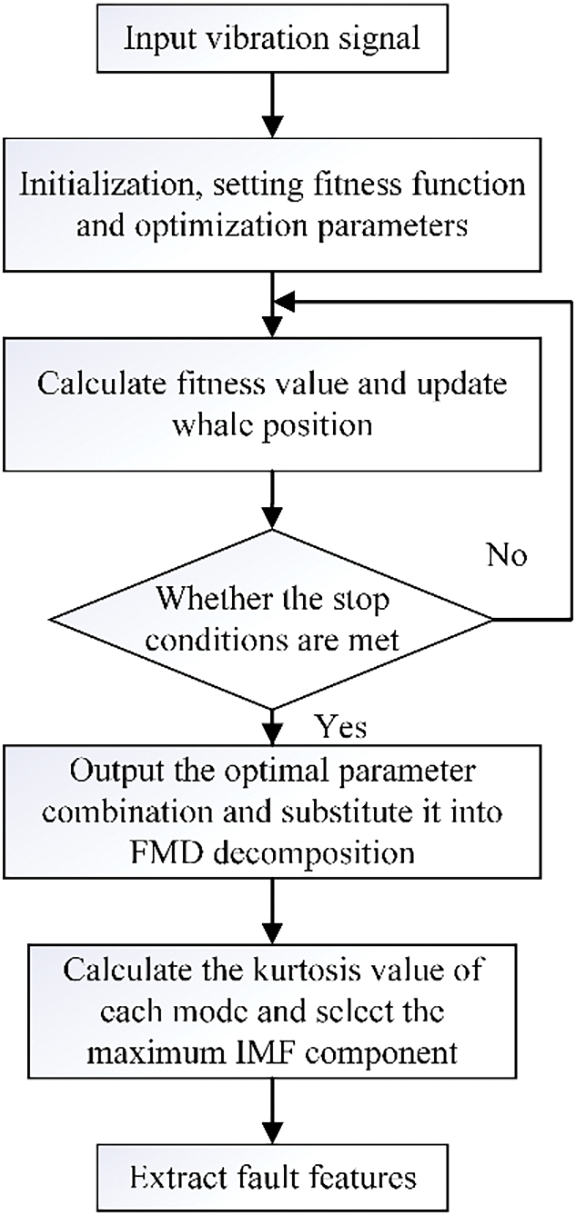
Figure 1: Flow chart of LMWOA-FMD algorithm
3 Fault Diagnosis Based on Improved DBN
DBN is made up of multiple RBM stacks and a classifier at the top level. Each RBM is composed of a visible layer and a hidden layer. The visible layer and the hidden layer are connected by weights, and the neurons in the same layer are independent of each other. The structure of RBM is shown in Fig. 2.
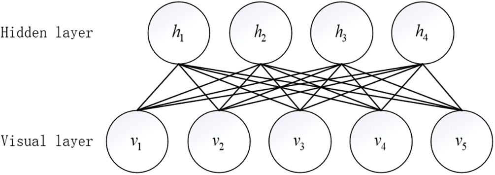
Figure 2: RBM structure diagram
DBN continuously extracts the relevant characteristics of the previous output layer through RBM, which realizes the step-by-step training from the bottom to the top. In the fine-tuning process of the whole DBN structure, in addition to training, the optimal mapping between each RBM is obtained. It also needs to use the BP algorithm to gradually propagate the error between the output value and the expected value from the top layer to the bottom layer. The structure of DBN is shown in the Fig. 3.
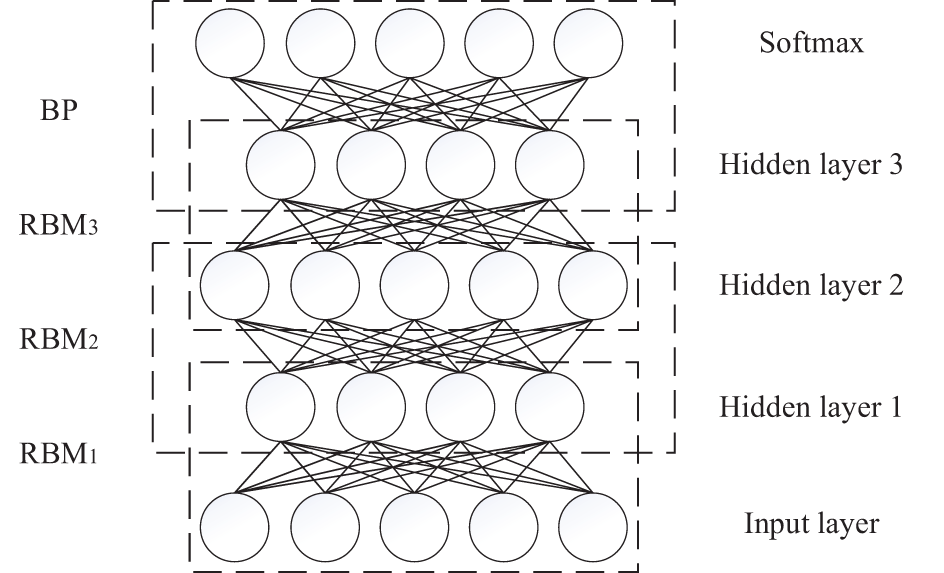
Figure 3: DBN structure diagram
During the training process, the state of neurons in the visible layer of RMB is expressed as
where
When all parameters are determined, Eq. (7) can be expressed by the joint probability distribution function between the visible layer and the hidden layer, as shown in Eq. (8):
Because there is no correlation between neurons in each layer, it is necessary to use activation function to calculate whether neurons are activated. The commonly used activation functions in deep learning include Sigmaid, Tanh, ReLU, etc. When sigmoid and tanh functions approach positive and negative infinity, the gradient disappears and the weight update speed decreases. The ReLU function solves the problem of vanishing gradients, but the derivative remains 0 at negative values. It is prone to neuronal necrosis. Hard swish function not only guarantees the advantages of ReLU function but also overcomes the computational defects. It is smoother and has a faster rate of convergence speed [31]. Hard swish function expression is:
The probability of conditional distribution for visible and hidden layers is:
The original Sigmoid function has been replaced by a Hard swish function in this paper. This can solve the problem that the gradient disappears and the weight update speed decreases. Therefore, the accuracy of the deep belief network is improved.
3.3 LMWOA-IDBN Diagnosis Model
At different time scales, multiscale entropy can calculate the complexity of signals. It has good anti-interference and anti-noise effects. When a signal is more complex and the fluctuation is greater, the multiscale entropy is greater. MSE sets the embedding dimension to 2, the maximum value of multi-scale factors is 20 and the similarity dimension is taken as 0.15 std. The multi-scale entropy and envelope spectrum of FMD processed signals are combined to form a new fault feature data set. It is split into training and testing sets in a 7:3 ratio with input to the IDBN.
The hidden layers and the number of neurons in each layer of the deep belief networks have a significant impact on the performance of the neural network. The performance of the neural network is strongly influenced by these main characteristic parameters. For instance, if the number of neuron nodes in the hidden layer is too small, it cannot produce enough connection weight combinations to learn. A network structure will be generalized if the number of concealed layers is too large. The Learning rate will affect the rate of convergence and final accuracy of the network. An optimal parameter value should be found to obtain the most suitable diagnostic model for data classification or prediction. The number of hidden layer nodes
Step 1: input the processed data set, divide it into training data set and test data set according to 7:3, and initialize IDBN parameters.
Step 2: use the training data set to update the whale position iteratively, train the IDBN model, and seek the optimal parameter combination
Step 3: using the error of DBN as the fitness function of the algorithm, calculate the fitness value and update the whale position. Judge whether the current stop condition is met. If not, return to step 2 and continue iteration.
Step 4: output the optimal parameter combination and build the IDBN diagnosis model.
Step 5: input the test data set into the IDBN diagnostic model and output the final classification results.
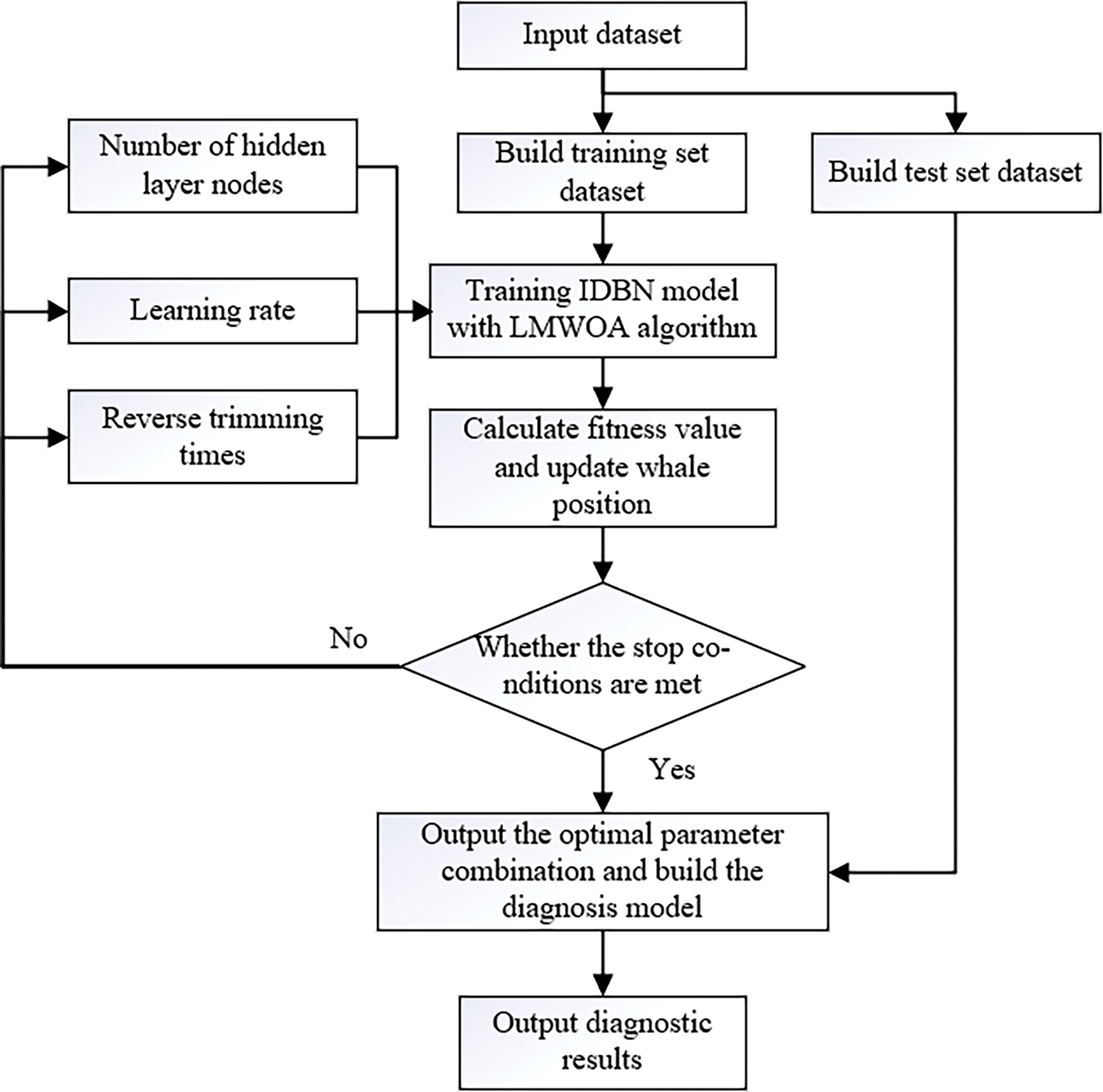
Figure 4: LMWOA-IDBN diagnostic flowchart
4 Experimental Signal Analysis
The data of the experiment is from the bearing data set provided by CWRU [32]. The bearing type is SKF6205-2RS. The experiment collected signals of inner ring failure, outer ring failure, rolling element failure, and normal state. The fault diameters are divided into 0.1778, 0.3556, and 0.5334 mm. The power of the load motor is 0,1,2 and 3 hp, respectively. The experimental platform is shown in Fig. 5. To verify the noise resistance of the method, a −5 dB Gaussian white noise was added to the experimental dataset.
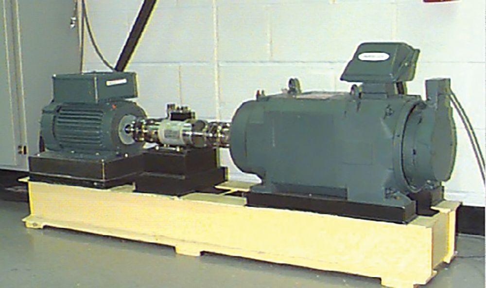
Figure 5: Simulation experimental device of CWRU
Taking the 0.1778 mm single point inner ring fault signal under 0 hp load as an example, select 2048 data points with a signal length. PSO, WOA, and LMWOA are used to optimize FMD parameters respectively. Set the number of iterations to 10 and the population to 15. Fig. 6 shows the change in the fitness function value. LMWOA converges when the number of iterations reaches 6. The final fitness function value found by the three optimization methods is 7.013. The convergence speed of LMWOA is better than the other two methods.
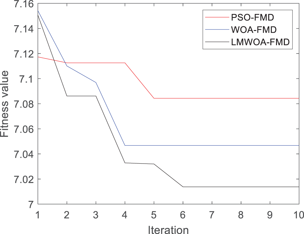
Figure 6: Fitness function value change of experimental inner ring fault signal in the experiment
After PSO optimization,
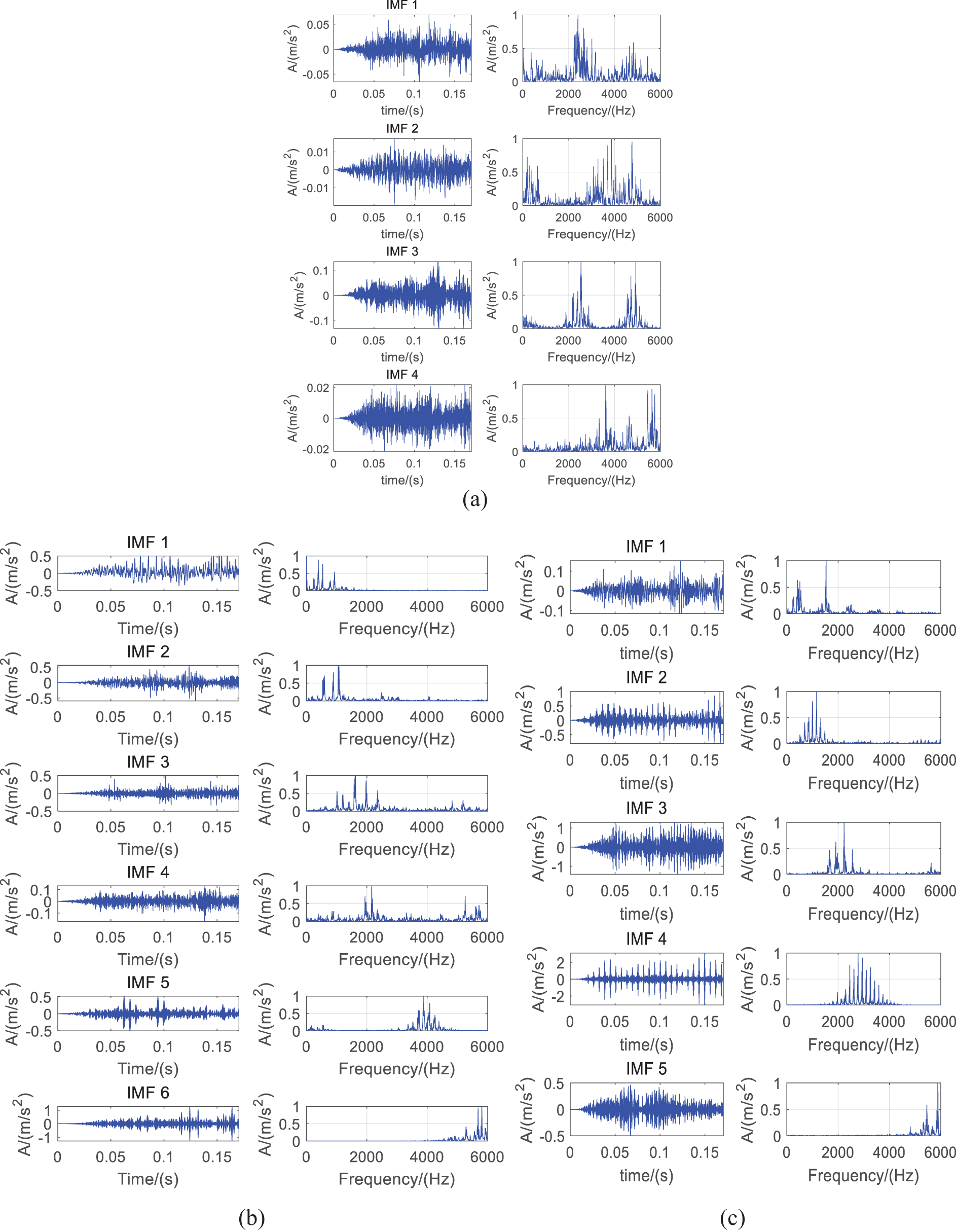
Figure 7: Result of outer ring fault signal in the experiment: (a) PSO-FMD (b) WOA-FMD (c) LMWOA-FMD
For an envelope demodulation analysis, select the IMF component that has the largest kurtosis value, and its results are presented in Fig. 8. According to the calculation theory, the fault frequency is
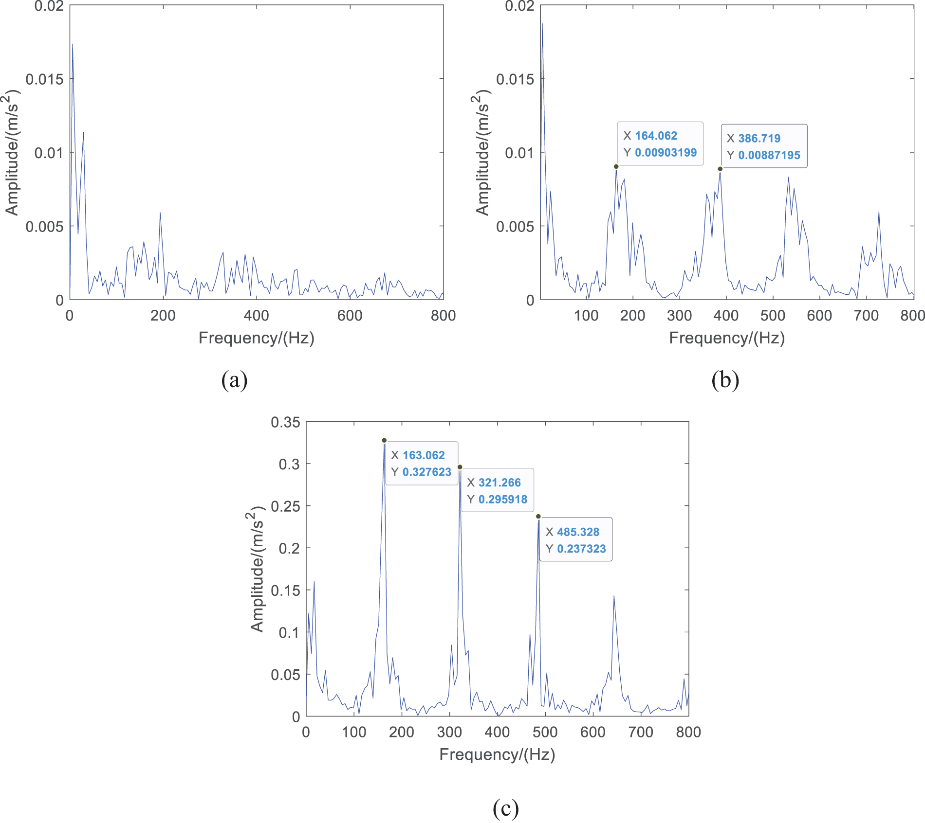
Figure 8: Envelope spectrum of inner circle fault signal in Experiment: (a) result by LMWOA-FMD (b) result by FMD (c) original signal
Further, select FFR to compare the two methods. If the value of FFR is larger, it indicates that the component contains more periodic impact components. After calculation, the FFR values of the WOA-FMD, and LMWOA-FMD are 0.019, and 0.137, respectively. It is proved that the fault frequency and multiple frequencies extracted by the LMWOA FMD method are more obvious in the envelope spectrum. The fault features can be better extracted after parameter optimization.
4.3 Experiments on Different Load States
The data sets of different load states are fault signals and normal signals of three loads (0, 1, 2 hp) under 0.01778 mm fault diameter, with a total of 12 types. Select 100 samples for each type of signal, the sample length is 2048.
IDBN sets two layers of RBM, the number of iterations of each RBM is 300, the momentum factor is 0.5, and the initial learning rate is 0.1. Data set 1 is processed and input into the IDBN optimized by LMWOA, WOA, and PSO algorithms, respectively. Set the population size to 20 and the maximum number of iterations to 15. The fitness value of IDBN changes as shown in Fig. 9. When the number of iterations reaches 10, LMWOA has converged. Through searching, the fitness value obtained is 0.019. The fitness values of PSO and WOA were 0.047, which failed to jump out of the local optimum. It is further proved that LMWOA can solve the problem of falling into local optimization and ensure the accuracy of the optimization results.
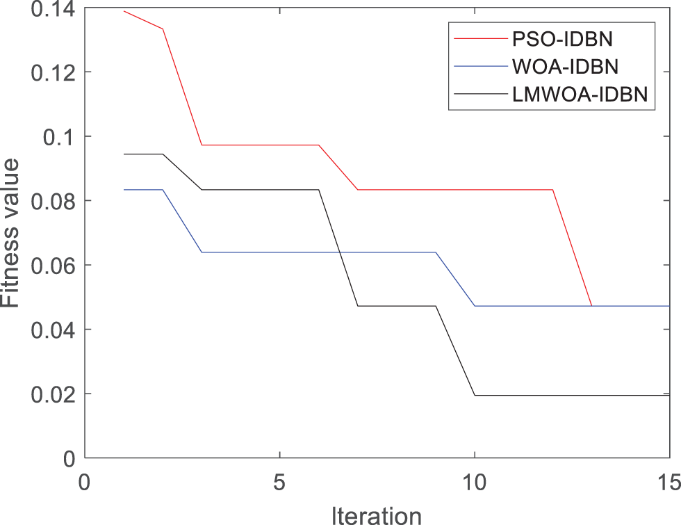
Figure 9: Fitness curve of different optimization methods under different loads
After optimization by LMWOA parameters, the learning rate is 0.044, the number of reverse fine-tuning is 357, and the optimal number of hidden layer nodes is [82,39]. The final diagnosis result is shown in Fig. 10. The fault accuracy of the LMWOA-FMD-IDBN model under different load conditions is 98%. It can better distinguish 12 kinds of bearing signals under different loads.
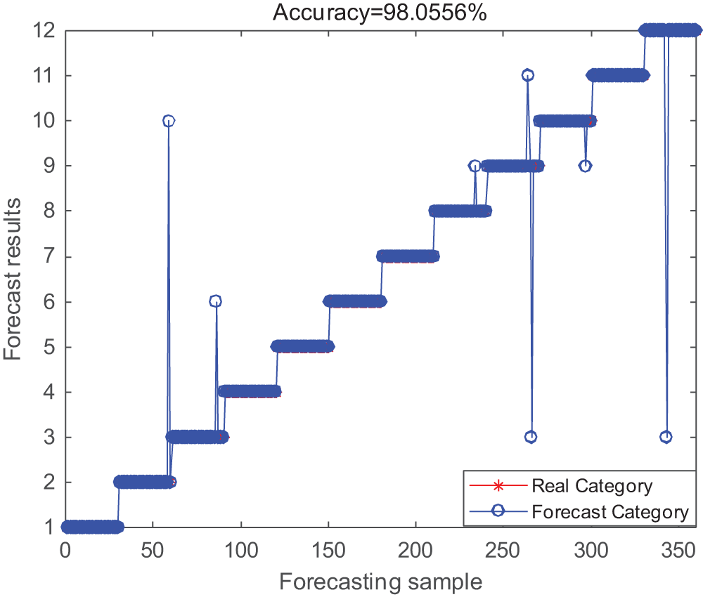
Figure 10: LMWOA-FMD-IDBN fault classification results under different loads
In order to demonstrate the powerful ability of IDBN in automation to extract valuable information from the original feature set, the T-SNE method was used to study the layer-by-layer feature learning process in the experiment.
As shown in Fig. 11a, the original features of the 12 categories are distributed in space, and most of them overlap each other, so it is difficult to distinguish data categories by them. Figs. 11b and 11c show the features of the first and second layers, which are more recognizable than the original features. But the hidden layer extracts the main features from the original data. They are similar in many aspects, which is not enough to distinguish each category. After the softmax layer is classified, almost all of them can be separated, and the results are shown in the Fig. 11d. The results show that IDBN has good ability of feature extraction and fault classification.
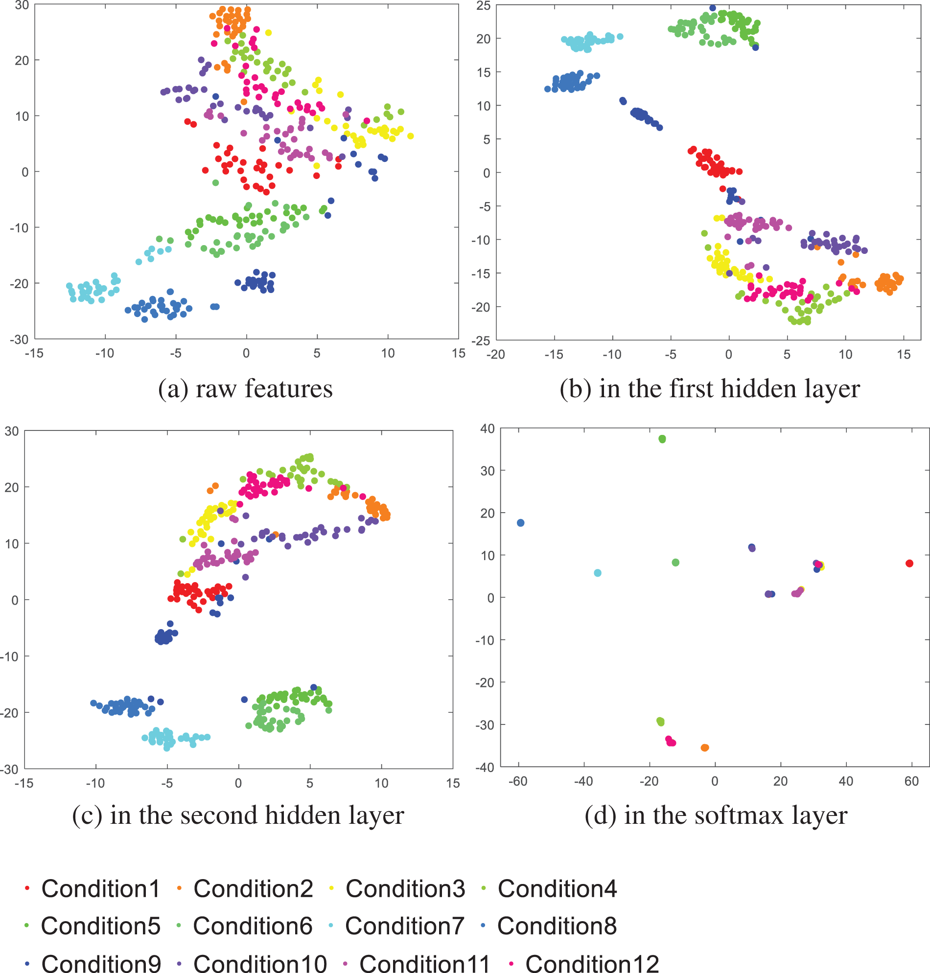
Figure 11: Visualization results of T-SNE under different loads
To further verify the advantages of this method, the DBN using the Sigmoid activation function will be compared. After parameter optimization, the training set accuracy curves of two different activation functions are shown in Fig. 12. The results show that the IDBN using Hard Swish activation function converges when the number of fine-tuning is 357. It has a fast-training speed, and the training accuracy is 98.7%. The curve of DBN fluctuates greatly and converges slowly. When the number of fine adjustments is 500, the convergence value just reaches 95.1%. The IDBN using Hard swish activation function has no fluctuation in the convergence curve and can converge faster, which shows that the method has good stability.
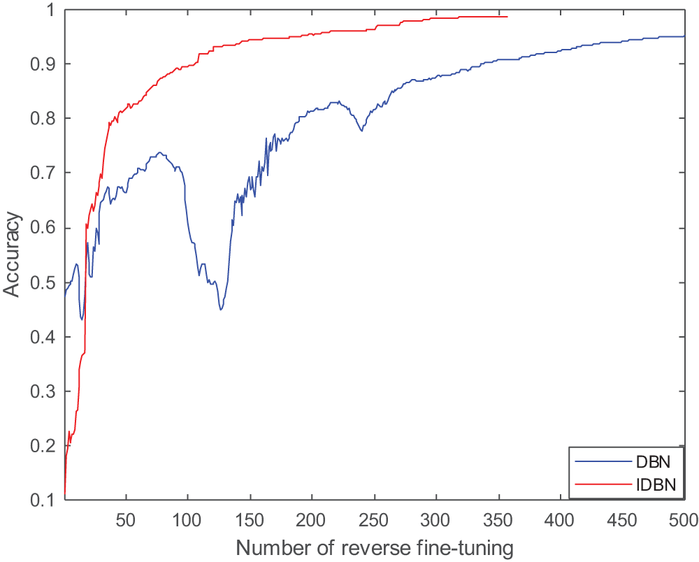
Figure 12: Training curves of different activation functions under different loads
To verify the effectiveness of the presented model in rolling bearing fault diagnosis, LMWOA-SVM, DenseNet, ResNet, IDBN, and other methods are selected for comparative experiments. DenseNet and ResNet methods use CWT to convert into two-dimensional images set the learning rate to 0.0001 and train 50 times. Manually set the learning rate of IDBN to 0.01, the number of reverse fine adjustments to 1000, and the number of hidden layer parameter nodes to [120,60]. To ensure the reliability of the experiment, 10 tests are conducted on each model on two datasets. The average of the 10 tests is taken, the results are shown in Fig. 13.
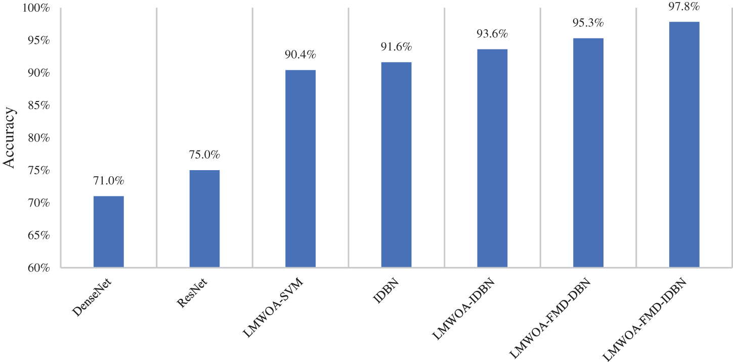
Figure 13: Average accuracy of different diagnostic models under different loads
In the figure, IDBN using LMWOA parameter optimization and Hard swish activation function has the highest accuracy. The average accuracy is 97.8%. Compared with other methods, the diagnosis error of this model is smaller. At the same time, after LMWOA-FMD processing, the noise interference is successfully removed. The accuracy of the model has been significantly improved. The Hard swish activation function not only improves the training speed but also improves the accuracy of the test set. The superiority of this method in rolling bearing fault diagnosis under different loads is verified.
4.4 Experiments with Different Degrees of Damage
The dataset with different degrees of damage includes three types of fault signals (0.1778, 0.3556, and 0.5334 mm) and normal signals under 0 hp load, with a total of 10 types. Select 100 samples for each type of signal, the sample length is 2048.
Similarly, the input of the second dataset was processed by the LMWOA-FMD method into the IDBN optimized by the LMWOA, WOA, and PSO algorithms. Set the overall size to 20 and the maximum number of iterations to 15. The changes in fitness values of the three methods are shown in Fig. 14. The final fitness values of PSO and WOA were both 0.04. LMWOA found this result for the sixth time and successfully jumped out. Finally, the optimal solution is found at the ninth time. The final fitness value was 0.017. It is proved again that LMWOA has better searchability and the ability to jump out of the local optimum. It can accurately find the optimal parameters of IDBN and improve the accuracy of the model.

Figure 14: Fitness curves of different optimization methods under different damage diameters
After optimization by LMWOA parameters, the learning rate is 0.056, the number of reverse fine-tuning is 263, and the optimal number of hidden layer nodes is [112,102]. The final diagnosis result is shown in Fig. 15. The fault accuracy of the LMWOA-FMD-IDBN model under different degrees of damage is 98.3%. It can effectively distinguish fault types with different loss diameters and perform diagnostic classification.
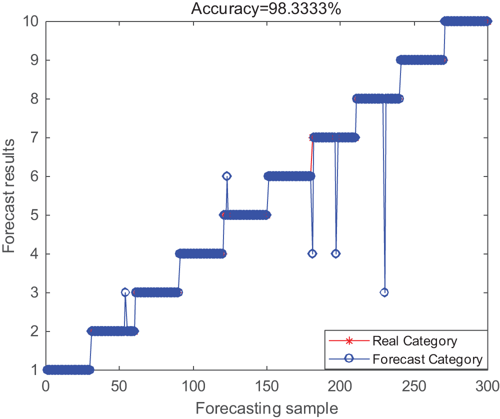
Figure 15: LMWOA-FMD-IDBN fault classification results under different damage diameters
The final classification layer of DBN and IDBN in the experiment is visualized by t-SNE method, and the results are shown in Fig. 16. Most of the 10 types in DBN overlap, while IDBN has better classification aggregation and no large area of overlap, which shows that IDBN has better ability of feature extraction and fault classification.
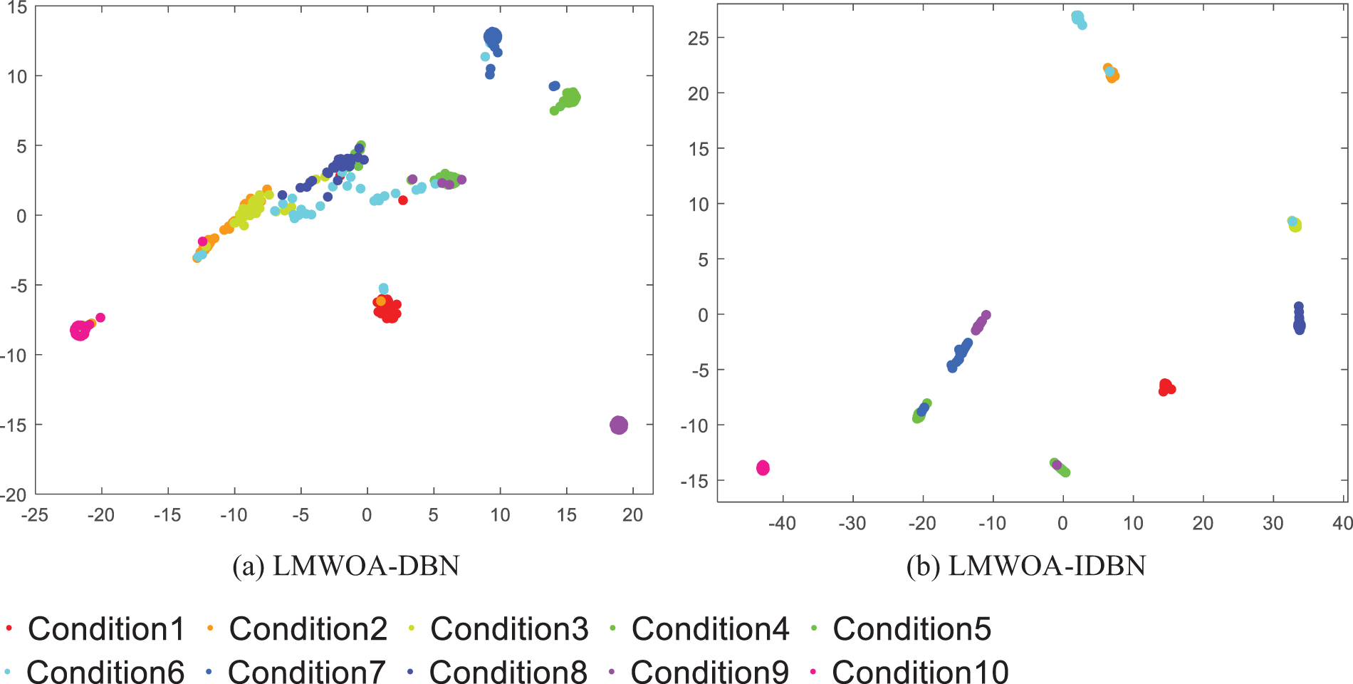
Figure 16: Visualization results of T-SNE under different damage diameters
The training curves of DBN using Sigma activation function and IDBN using Hard swish activation function are shown in Fig. 17. The training speed of the improved IDBN has been significantly improved, and the diagnostic accuracy is far greater than that of DBN. It shows that the Hard swish activation function plays a good role in the training process of DBN.
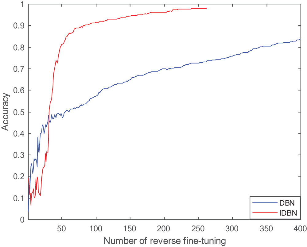
Figure 17: Training curves of different activation functions under different damage diameters
To verify the effectiveness of the proposed model in fault diagnosis of rolling bearings, LMWOA-SVM, DenseNet, ResNet, IDBN, and other methods are still selected for comparative experiments. The parameter setting method is the same as the last experiment. To ensure the reliability of the experiment, 10 tests are conducted on each model on two datasets. The average of the 10 tests is taken, and the results are shown in Fig. 18.
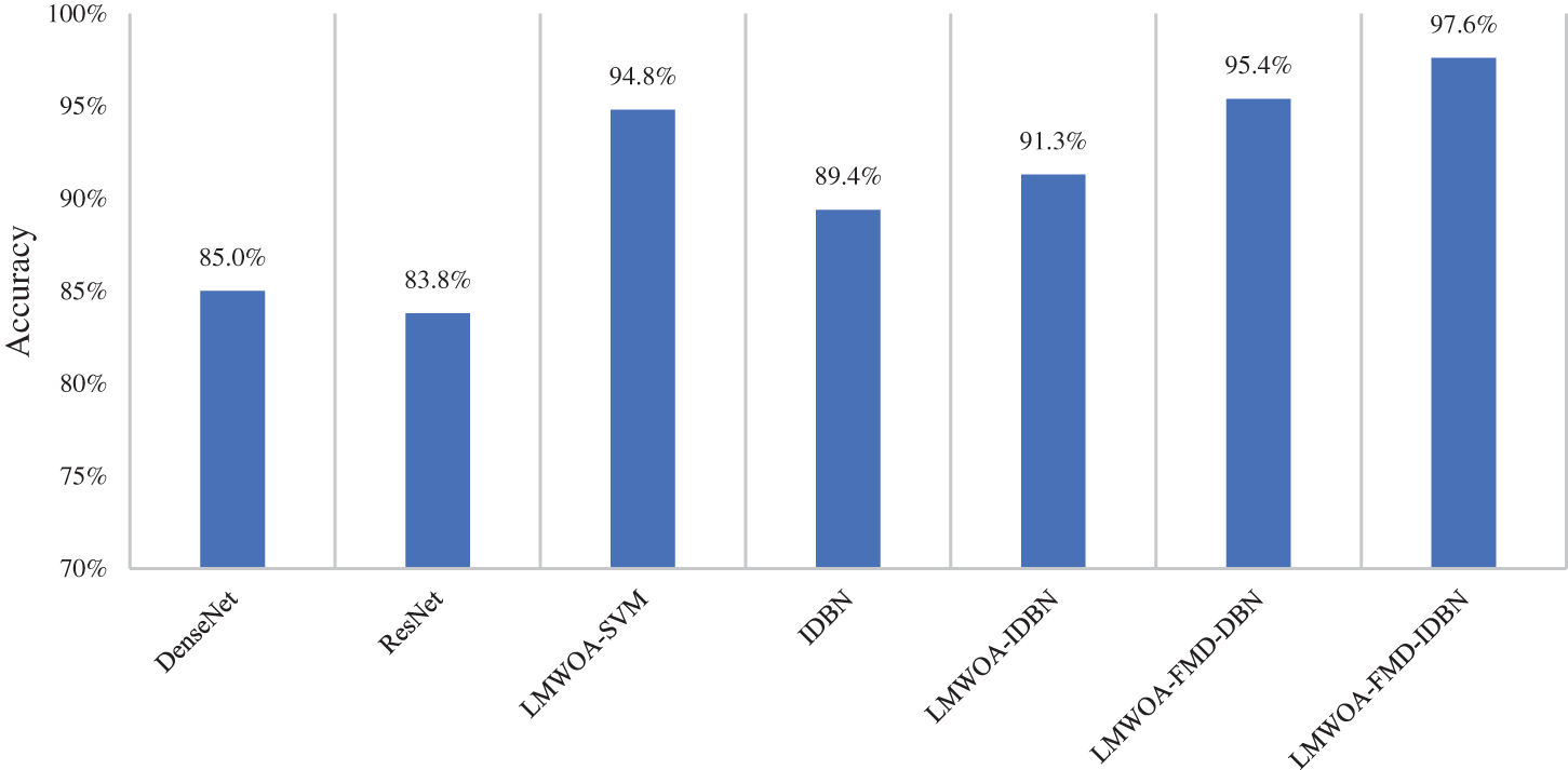
Figure 18: Average accuracy of different diagnostic models under different damage diameters
The average diagnostic accuracy of the LMWOA-FMD-IDBN model was 97.6%, which was higher than that of other methods. Compared with the signal without FMD decomposition, this method has significantly improved, indicating that this method has better anti-noise ability. The improved DBN using Hard swish activation function can speed up the training speed and improve the diagnosis accuracy.
Aiming at the adaptation problem of FMD and DBN parameters, as well as the phenomenon of DBN activation function gradient disappearance and neuron necrosis. The LMWOA-FMD-IDBN bearing fault diagnosis method is proposed. Lévy flight and adaptive weight are introduced in WOA. The parameters of FMD and IDBN using the Hard swish activation function are optimized by using LMWOA. Through experiments and comparisons, the following conclusions have been drawn:
(1) The LMWOA algorithm can avoid getting stuck in local optima during the parameter optimization process of FMD and IDBN and can converge to the optimal parameters faster, achieving parameter adaptation. Through experimental comparisons under different conditions, the accuracy of the optimized IDBN has been improved by 6.2% and 8.2%, respectively. In the presence of noise interference, it can ensure the extraction of more obvious fault features and more accurate fault diagnosis accuracy.
(2) Under different load conditions and different damage diameters, the IDBN using the Hard swish activation function and the original DBN have faster training speeds during the training process. In the test set, the diagnostic accuracy of IDBN has been significantly improved by 2.5% and 2.2%, respectively. Compared with LMWOA-SVM, RESNET, and other methods, this method has the highest accuracy, reaching 97.8% and 97.6%. It has higher diagnostic accuracy and can better distinguish fault types.
Acknowledgement: None.
Funding Statement: The research was supported by Central Guidance on Local Science and Technology Development Fund of Hebei Province (Grant No. 226Z1906G), Hebei University Science and Technology Research Youth Fund Project (QN2023188).
Author Contributions: The authors confirm contribution to the paper as follows: study conception and design: Guangfei Jia; data collection: Yanchao Meng; analysis and interpretation of results: Guangfei Jia, Zhiying Qin; draft manuscript preparation: Yanchao Meng. All authors reviewed the results and approved the final version of the manuscript.
Availability of Data and Materials: The authors confirm that the data supporting the findings of this study are available within the article.
Conflicts of Interest: The authors declare that they have no conflicts of interest to report regarding the present study.
References
1. Wei, Y., Li, Y. Q., Xu, M. Q., Huang, W. H. (2019). A review of early fault diagnosis approaches and their applications in rotating machinery. Entropy, 21(4), 409. https://doi.org/10.3390/e21040409 [Google Scholar] [CrossRef]
2. Jiang, H. K., Li, C. J., Li, H. X. (2013). An improved EEMD with multiwavelet packet for rotating machinery multi-fault diagnosis. Mechanical Systems and Signal Processing, 36(2), 225–239. https://doi.org/10.1016/j.ymssp.2012.12.010 [Google Scholar] [CrossRef]
3. Jin, Z. Z., He, D. Q., Wei, Z. X. (2022). Intelligent fault diagnosis of train axle box bearing based on parameter optimization VMD and improved DBN. Engineering Applications of Artificial Intelligence, 110(7), 104713. https://doi.org/10.1016/j.engappai.2022.104713 [Google Scholar] [CrossRef]
4. Feng, Z., Chen, X., Wang, T. (2017). Time-varying demodulation analysis for rolling bearing fault diagnosis under variable speed conditions. Journal of Sound and Vibration, 400(2), 71–85. https://doi.org/10.1016/j.jsv.2017.03.037 [Google Scholar] [CrossRef]
5. Wang, J. X., Zhan, C. S., Li, S. P., Zhao, Q. C., Liu, J. Q. (2022). Adaptive variational mode decomposition based on Archimedes optimization algorithm and its application to bearing fault diagnosis. Measurement, 191(1–2), 110798. https://doi.org/10.1016/j.measurement.2022.110798 [Google Scholar] [CrossRef]
6. Huang, N., Shen, Z., Long, S. (1998). The empirical mode decomposition and the Hilbert spectrum for non-linear and non-stationary time series analysis. Proceedings of the Royal Society of London. Series A: Mathematical, Physical and Engineering Sciences, 454(1971), 903–995. https://doi.org/10.1098/rspa.1998.0193 [Google Scholar] [CrossRef]
7. Li, H. G., Hu, Y., Li, F. C., Meng, G. (2017). Succinct and fast empirical mode decomposition. Mechanical Systems and Signal Processing, 85(3), 879–895. https://doi.org/10.1016/j.ymssp.2016.09.031 [Google Scholar] [CrossRef]
8. Zhang, K., Xu, Y. G., Chen, P. (2021). Feature extraction by enhanced analytical mode decomposition based on order statistics filter. Measurement, 173(1), 108620. https://doi.org/10.1016/j.measurement.2020.108620 [Google Scholar] [CrossRef]
9. Lei, Y. G., He, Z. J., Zi, Y. Y. (2009). Application of the EEMD method to rotor fault diagnosis of rotating machinery. Mechanical Systems and Signal Processing, 23(4), 1327–1338. https://doi.org/10.1016/j.ymssp.2008.11.005 [Google Scholar] [CrossRef]
10. Liu, F., Gao, J., Liu, H. (2020). The feature extraction and diagnosis of rolling bearing based on CEEMD and LDWPSO-PNN. IEEE Access, 8, 19810–19819. https://doi.org/10.1109/ACCESS.2020.2968843 [Google Scholar] [CrossRef]
11. Dragomiretskiy, K., Zosso, D. (2014). Variational mode decomposition. IEEE Transactions on Signal Processing, 62(3), 531–544. https://doi.org/10.1109/TSP.2013.2288675 [Google Scholar] [CrossRef]
12. Ding, J., Huang, L., Xiao, D., Li, X. (2020). GMPSO-VMD algorithm and its application to rolling bearing fault feature extraction. Sensors, 20(7), 1946. https://doi.org/10.3390/s20071946 [Google Scholar] [CrossRef]
13. Miao, Y. H., Zhang, B. Y., Li, C. H. (2022). Feature mode decomposition: New decomposition theory for rotating machinery fault diagnosis. IEEE Transactions on Industrial Electronics, 70(2), 1949–1960. https://doi.org/10.1109/TIE.2022.3156156 [Google Scholar] [CrossRef]
14. Yan, X. A., Jia, M. P. (2022). Bearing fault diagnosis via a parameter-optimized feature mode decomposition. Measurement, 203(2), 112016. https://doi.org/10.1016/j.measurement.2022.112016 [Google Scholar] [CrossRef]
15. Liu, J. Y., Zhu, B. L. (2012). The application of particle swarm optimization algorithm in the extremum optimization of nonlinear function. IEEE 12th International Conference on Computer and Information Technology, pp. 286–289. [Google Scholar]
16. Jia, G. F., Meng, Y. C. (2023). Study on fault feature extraction of rolling bearing based on improved WOA-FMD algorithm. Shock and Vibration, 5097144. https://doi.org/10.1155/2023/5097144 [Google Scholar] [CrossRef]
17. Zheng, H. B., Zhang, Y. Y., Liu, J. F., We, H., Zhao, J. H. (2018). A novel model based on wavelet LS-SVM integrated improved PSO algorithm for forecasting of dissolved gas contents in power transformers. Electric Power Systems Research, 15, 196–205. https://doi.org/10.1016/j.epsr.2017.10.010 [Google Scholar] [CrossRef]
18. Xiao, M. H., Zhang, W., Wen, K., Zhu, Y., Yiliyasi, Y. (2021). Fault diagnosis based on BP neural network optimized by beetle algorithm. Chinese Journal of Mechanical Engineering, 34, 119. https://doi.org/10.1186/s10033-021-00648-2 [Google Scholar] [CrossRef]
19. Rajeswari, C., Sathiyabhama, B., Devendiran, S., Manivannan, K. (2014). Bearing fault diagnosis using wavelet packet transform hybrid PSO and support vector machine. Procedia Engineering, 97(5), 1772–1783. https://doi.org/10.1016/j.proeng.2014.12.329 [Google Scholar] [CrossRef]
20. Niu, G. X., Wang, X., Golda, M. (2021). An optimized adaptive PReLU-DBN for rolling element bearing fault diagnosis. Neurocomputing, 445(12), 26–34. https://doi.org/10.1016/j.neucom.2021.02.078 [Google Scholar] [CrossRef]
21. Guo, L. H., Yang, L. M., Peng, Y. F., Guo, Y. (2022). Fault identification of low-speed hub bearing of crane bas-ed on MBMD and BP neural network. Shock and Vibration, 2022, 500523. https://doi.org/10.1155/2022/5005263 [Google Scholar] [CrossRef]
22. Zhang, X. Y., Liang, Y. T., Zhou, J. Z., Zang, Y. (2015). A novel bearing fault diagnosis model integrated permutation entropy, ensemble empirical mode decomposition and optimized SVM. Measurement, 69, 164–179. https://doi.org/10.1016/j.measurement.2015.03.017 [Google Scholar] [CrossRef]
23. Dong, Z., Zheng, J., Huang, S., Pan, H., Liu, Q. (2019). Time-shift multi-scale weighted permutation entropy and GWO-SVM based fault diagnosis approach for rolling bearing. Entropy, 21(6), 621. https://doi.org/10.3390/e21060621 [Google Scholar] [CrossRef]
24. Wang, Z. Y., Li, G. S., Yao, L. G., Cai, Y. X., Lin, T. X. et al. (2023). Intelligent fault detection scheme for constant-speed wind turbines based on improved multiscale fuzzy entropy and adaptive chaotic Aquila optimization-based support vector machine. ISA Transactions, 138(6), 582–602. https://doi.org/10.1016/j.isatra.2023.03.022 [Google Scholar] [CrossRef]
25. Wang, Z. Y., Yao, L. G., Cai, Y. W., Zhang, J. (2020). Mahalanobis semi-supervised mapping and beetle antennae search based support vector machine for wind turbine rolling bearings fault diagnosis. Renewable Energy, 155(2), 1312–1327. https://doi.org/10.1016/j.renene.2020.04.041 [Google Scholar] [CrossRef]
26. Jürgen, S. (2015). Deep learning in neural networks: An overview. Neural Networks, 61(3), 85–117. https://doi.org/10.1016/j.neunet.2014.09.003 [Google Scholar] [CrossRef]
27. Xu, H. F., Wang, X., Huang, J. F., Zhang, F. B., Chu, F. L. et al. (2024). Semi-supervised multi-sensor information fusion tailored graph embedded low-rank tensor learning machine under extremely low labeled rate. Information Fusion, 105, 102222. [Google Scholar]
28. Hinton, G. E., Salakhutdinov, R. R. (2006). Reducing the dimensionality of data with neural networks. Science, 313(5786), 504–507. https://doi.org/10.1126/science.1127647 [Google Scholar] [CrossRef]
29. Shao, H. D., Jiang, H. K., Wang, F. A., Wang, Y. N. (2017). Rolling bearing fault diagnosis using adaptive deep belief network with dual-tree complex wavelet packet. ISA Transactions, 69(5), 187–201. https://doi.org/10.1016/j.isatra.2017.03.017 [Google Scholar] [CrossRef]
30. Mirjalili, S., Lewis, A. (2016). The whale optimization algorithm. Advances in Engineering Software, 95(12), 51–67. https://doi.org/10.1016/j.advengsoft.2016.01.008 [Google Scholar] [CrossRef]
31. Howard, A., Sandler, M., Chu, G., Chen, L. C., Chen, B. et al. (2019). Searching for MobileNetV3. IEEE/CVF International Conference on Computer Vision, pp. 1314–1324. https://doi.org/10.1109/ICCV.2019.00140 [Google Scholar] [CrossRef]
32. Smith, W. A., Randall, R. B. (2015). Rolling element bearing diagnostics using the case western reserve university data: Rolling element bearing diagnostics using the case western reserve university data: A benchmark study benchmark study. Mechanical Systems and Signal Processing, 64–65, 100–131. https://doi.org/10.1016/j.ymssp.2015.04.021 [Google Scholar] [CrossRef]
Cite This Article
 Copyright © 2024 The Author(s). Published by Tech Science Press.
This work is licensed under a Creative Commons Attribution 4.0 International License , which permits unrestricted use, distribution, and reproduction in any medium, provided the original work is properly cited.
 Downloads
 Citation Tools