Identification of Damage in Steel‒Concrete Composite Beams Based on Wavelet Analysis and Deep Learning

1  Introduction

Steel-concrete composite beams effectively exploit the advantages of steel (tensile strength) and concrete (compressive strength), representing commonly employed structural configurations for large-scale bridges, particularly arch bridges, cable-stayed bridges, and suspension bridges [1]. These steel-concrete composite beams have advantages, such as small structural height, low self-weight, high load-bearing capacity, substantial stiffness, savings in formwork procedures and templates, reduced on-site wet construction, fast construction speed, and overall superior performance. However, due to inherent material limitations, several unavoidable issues manifest as follows: 1) Concrete subjected to negative bending moments is susceptible to cracking; 2) inadequate maintenance of steel beams can lead to corrosion after paint degradation; and 3) concrete cracking may result in shear force connection component failure. These three factors impact the load-bearing capacity and durability of steel-concrete composite beams. Hence, it is necessary to employ precise testing methods for damage identification when steel-concrete composite beams are in the operational phase, facilitating early discovery and mastery of structural damage conditions while ensuring the safety and reliability of bridge structures.

Scholars both domestically and internationally have conducted extensive research and analysis on damage identification for bridges. Because the dynamic characteristics of a structure are sensitive to damage [2], traditional identification methods rely primarily on variations in the dynamic properties of structures (such as frequency, vibration modes, curvature modes, and strain modes) to infer the presence of damage [3–7]. Nonetheless, the frequency of steel-concrete composite beams is significantly affected by temperature, the curvature mode is sensitive to specific types of damage, and the strain modes necessitate an extensive array of sensors for data acquisition, with the strain gauges and accelerometer sensors exhibiting weak resistance to interference.

In recent years, researchers have succeeded in extracting damage information from vibration signals generated by structures during excitation, such as via wavelet analysis. Wavelet analysis, also known as wavelet transformation, is a rapidly evolving field in applied mathematics and engineering. Researchers can use it to perform multiscale joint analysis of data in the time domain and frequency [8]. Moreover, wavelet analysis accurately has revealed the location and extent of localized damage in plates and beams [9–11]. However, wavelet analysis for damage identification still requires manual the manual selection of features of the vibration signal, which does affect the accuracy of the identification.

With the rapid advancement of computer technology, more intelligent feature extraction methods, such as deep learning, have been utilized in structural damage identification. The recognition method, which is based on deep learning, can automatically extract features and input them into a classifier for classification rather than relying on manual feature selection. Compared to those of shallow neural networks, deep learning architectures can provide higher-level representations of features. In addition, deep learning techniques, such as image classification, object detection, semantic segmentation, and instance segmentation, typical network models, such as convolutional neural network (CNN), MobileNet, residual network (ResNet), adaptive prototype alignment network (AP-Net), U-Net, Visual Geometry Group Network (VGN), You Only Look Once (YOLO), and region-based fully convolutional network (R-FCN), have been used in conjunction with civilian engineering disease detection, Shi et al. [12] introduced a CNN-based model to monitor fatigue cracks in steel bridge decks. Zhuo et al. [13] proposed an innovative online diagnostic procedure using sound signals for identifying bolt connection damage in steel truss structures. Huynh [14] created a novel autonomous vision-based method for the detection of bolt looseness in splice connections. Utilizing convolutional neural networks (CNNs), Cha et al. [15] presented a method for concrete crack detection, achieving approximately 98% accuracy without traditional image processing techniques. Zhu et al. [16] employed transfer learning and CNNs in a vision-based approach for bridge defects detection, demonstrating a high accuracy of 97.8%, thus showcasing its superiority over manual inspections. Huang et al. [17] formulated a deep residual network model to classify concrete diseases, with an overall accuracy of 91.3% and a notable 97.6% accuracy in identifying rebar exposed diseases. Nie et al. [18] devised a framework combining artificial neural networks and Monte Carlo simulations for analyzing the fatigue reliability of steel bridges, effectively maintaining fatigue failure probability within 2.3%. Lu et al. [19] innovated a learning machine that integrates uniform design and support vector regression, serving as an alternative to time-consuming finite-element models. Sun et al. [20] introduced a Gaussian Bayesian Network (GBN)-based method for damage detection in steel truss bridges, utilizing strain monitoring data. Luo et al. [21] enhanced road damage detection with their E-EfficientDet network, surpassing traditional models like YOLOv5s and Faster R-CNN. Lastly, Guo et al. [22] leveraged a Kohonen neural network and long short-term memory (LSTM) neural network for bridge health monitoring, where the Kohonen method classifies data under normal conditions and detects outliers, while the LSTM method provides accurate predictions of future deflection values, aiding in the observation of changes in bridge structures.

However, in these studies, the predominant focus has been on structures of a single material, and there are relatively few research findings on the application of these techniques for damage identification in steel-concrete composite beams. This study aimed to develop a smarter, more convenient, and more accurate new method for damage identification in the field of steel-concrete composite beams.

The structural form of composite beams is different from that of steel beams or reinforced concrete beams; the damage state of composite beams is more complex (including that of concrete, steel beams, and shear connectors), and composite beams are more difficult to identify. Based on the above issues, an intelligent damage detection method for steel-concrete composite beams based on deep learning and wavelet analysis is proposed.

The main contributions of this work are as follows:

1. Establish a deep residual network model to obtain classifiers of seven concrete damage.

2. In this experiment, fiber grating strain sensor is used to collect test signals. The results show that the sensor has the advantages of low temperature strain, simple layout, high sensitivity, high resolution and strong anti-interference ability.

3. The comparison results show that the denoising performance of Harr wavelet is better than other functions, and the prediction accuracy of ResNet-50 model is better than other models.

4. The experiment indicates that the strain time domain signal can effectively reflect the damage information of the composite beam, and the deep learning model in this paper can accurately extract these damage features.

2  Relevant Theories and Identification Methods

Fiber Bragg grating sensors are widely used in the field of structural health monitoring because of their advantages, such as easy embedding and strong anti-interference ability [23], and because multiple fiber Bragg grating sensors can be connected in series into a sensor network for quasidistributed detection of structures [24]. In addition, compared with that of ordinary sensors, fiber grating sensors have better stability, thus improving the accuracy of damage identification [25,26].

Deep learning can directly extract high-level features from data and is different from traditional machine learning algorithms. Traditional machine learning methods usually separate problems into multiple subproblems, solve them one by one and finally combine the results of all subproblems to obtain the result. Deep learning is a direct end-to-end solution to this problem, without the need for an intermediate problem decomposition process, manual selection of features, or automatic extraction of features into the classifier for classification.

In this paper, six deep learning classification models, ResNet-18, ResNet-50, ResNet-101, InceptionV3, InceptionResNetV2, and MobileNetV2, are constructed. All these models are founded on convolutional neural networks (CNNs). Notably, the deep residual network (ResNet) introduces residual units to address the vanishing and exploding gradient challenges encountered during the training of deep neural networks. These residual units allow information to bypass certain layers, facilitating the ability of the network to effortlessly learn identity mappings, consequently enabling the training of deeper networks. The inception network is designed to extract features of varying scales and resolutions (i.e., a dataset composed of different-sized data) by using multiscale convolutions to capture features at different levels. Inception-ResNet, a fusion of Inception and ResNet, enhances model performance by combining the strengths of both. MobileNet is a lightweight convolutional neural network specifically tailored for mobile and embedded devices. It extends the receptive field of the network without increasing the parameter volume, effectively minimizing the loss of feature information extraction for smaller targets while enhancing the model computation speed.

The general idea of deep learning models performing classification tasks is basically the same. The network is trained by using labelled data samples to obtain the optimal model, which is subsequently tested with unlabelled data samples to validate its generalizability. The process flow is as shown in Fig. 1.

Figure 1: Deep learning training process

The principle of wavelet denoising: The signal is decomposed into subsignals of different scales by wavelet transform, and the subsignal is subsequently denoised by threshold processing. Finally, all the subsignals after noise reduction are reconstructed by the wavelet, and the final noise reduction signal is obtained. The median filter threshold function selected in this paper is a threshold selection method based on the data itself, which adaptively selects the threshold. The basic principle is to calculate the median of the absolute value of the subsignal of each scale and use this as the threshold. The threshold function is used to calculate the subsignals of each scale; a coefficient less than the threshold is set to 0, and a signal greater than or equal to the threshold is retained. The relevant formulas are as follows:

Decomposition​:C(a,b)=〈f(t),ψa,b(t)〉=∫−∞∞f(t) ψa,b*(t)dt(1)

Reconstruction​: f(t)=1Cψ∫−∞∞∫−∞∞C(a,b)​ ψa,b(t)dadba2 (2)

where f(t) is the original signal; C(a,b) is the decomposition coefficient; f(t) represents the eigenvalue under scale parameter a and migration parameter b; ψa,b(t) is the wavelet basis function; ψa,b*(t) is the conjugate complex form of the wavelet basis function; Cψ is a normalized constant used to ensure the conservation of energy in the reconstruction process; and da and db are the microelement changes in scale parameter a and migration parameter b, respectively.

The adaptive median filter threshold function is as follows:

g[n]={f[n]if|f[n]−m[n]|≤T1median(f[n−d],…,f[n+d])ifT1<|f[n]−m[n]|≤T2median(f[n−dmax],…,f[n+dmax])otherwise (3)

where g[n] is the output signal value; f[n] is the input signal value; m[n] is the current local median value, which represents the median signal value in the local region centred around sampling point n; T1 is a low threshold used to determine whether to keep the input signal value unchanged; T2 is the high threshold used to determine whether to use a larger local area for median calculation; median(f) is the median function used to calculate the median of a given dataset; f[n−d] , f[n+d] , f[n−dmax] and f[n+dmax] , respectively, represent the signal values in the left and right neighbourhood of the current sampling point; and d is the radius of the current neighbourhood, indicating the size of the current local area. In the initial stage of the algorithm, d = 1, and dmax is the maximum neighbourhood radius, which is used to limit the maximum range of the neighbourhood.

The technical flowchart of this paper is shown in Fig. 2.

Figure 2: Technology roadmap

3  Experimental Methodology

3.1 Test Specimens

The relevant design refers to the relevant provisions of steel-concrete composite beams in the Code for Design of Steel-Concrete Composite Bridges (GB 50917-2013). The design of the composite beam is as follows: The total length of the I-steel is 3 m, the material is Q235B, the net height of the section is 200 mm, the width of the upper and lower flanges is 150 mm, and the cross-sectional area is 37.92 cm2. The span of the concrete slab is 3000 mm, the material is C50, the width is 600 mm and the height is 80 mm. Eight steel rebars with a diameter of 8 mm are configured according to the section reinforcement rate of 0.84%, and a closed stirrup with a diameter of 6 mm is configured according to the stirrup rate of 0.475%. The space between the stirrups is 150 mm, and the steel bar material is HRB400. Shear nails made of ML15 are welded to the upper flange of the I-steel, arranged in 32 rows and 2 columns, for a total of 64 pieces. The spacing of the shear nails on the cross-section of the I-steel is 70 mm, and the longitudinal spacing along the I-beam steel-concrete composite beams is 90 mm. The specific dimensions are shown in Fig. 3 below. The specimen is shown in Fig. 4. The experimental subject comprises seven simply supported I-beam steel-concrete composite beams (hereafter referred to as composite beams).

Figure 3: Composite beam design drawing

Figure 4: Physical view of the combined beam specimen

3.2 Material Properties

In this paper, seven groups of 150 mm × 150 mm × 150 mm cubic concrete samples with a nominal strength of 50 MPa (Grade C50) were fabricated during casting to evaluate the concrete material properties. The test results reveal that the concrete has a 54.6 MPa cube compressive strength fcu, 44.5 MPa axial compressive strength fc, 4.8 MPa cube splitting strength ft and 42.6 GPa elastic modulus Ec.

The standard yield strength and standard tensile strength of the rebar and stirrups are 400 and 360 MPa, respectively. The product quality certificate provides the material properties, and the average yield strength and tensile strength of 9 rebars from the same batch are 479 and 547 MPa, respectively.

3.3 Test Instrumentation

The type of fiber grating strain sensor used was JFSS-04. This is a low-temperature sensitive fiber grating strain sensor. These sensors exhibit minimal variation of less than 1 microstrain for every 1°C temperature change. They possess a measurement range of ±800 με and offer an accuracy of 1% F.S. The fiber type used was SMF-28, and the resolution was 1 με. These sensors are designed for use within a temperature range of −30°C to 120°C, and they are protected with a 3 mm long casing. Table 1 shows some parameters of the sensor. A physical view of the sensor is shown in Fig. 5.

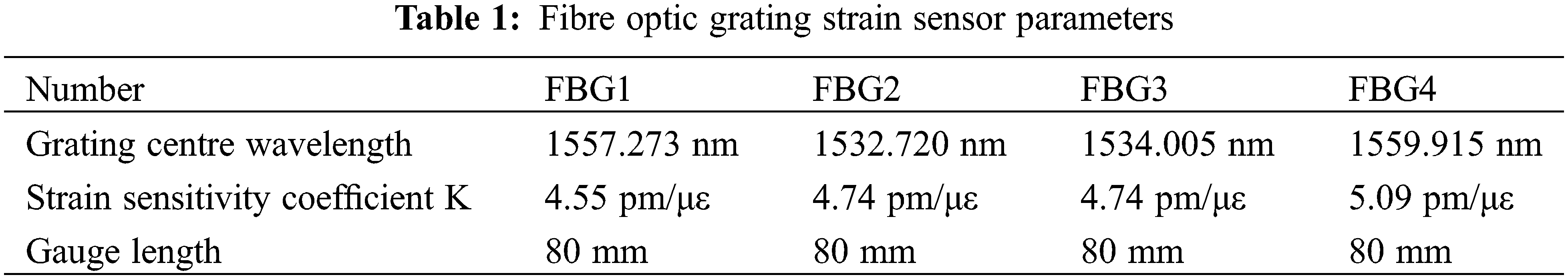
Figure 5: Photograph of the sensor

Since the structure has different temperature stresses and strains at different temperatures, the effect of temperature should be eliminated in this test. Low-temperature-sensitive fiber grating strain sensors of the same type were installed on steel plates and concrete blocks and placed in the same temperature field as the test beams. At the end of the test, the strains of the steel-concrete composite beams do not include the temperature strain.

The type of fiber grating demodulator used was SM130, manufactured by the MOI company in the United States. It converts changes in the wavelength of the fiber optic grating into strain vibration signals and provides four channels for simultaneous data acquisition. In this experiment, the sampling frequency was set at 1 kHz. The wavelength detection operates within the range of 1510 to 1590 nm, with a resolution less than 1 pm. Equipped with a standard Ethernet interface, the collected data are generally stored through the computer software. The SM130 fiber grating demodulator is shown in Fig. 6.

Figure 6: SM130 fiber grating demodulator

3.4 Damage Setting

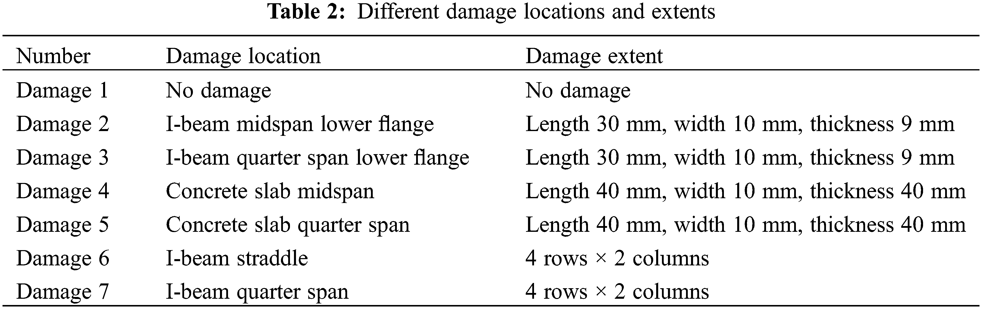
For composite beams in operation, the damaged components include steel beams, concrete slabs and shear nails, but the location and degree of damage cannot be completely simulated in the test. Therefore, typical mid-span and quarter-span damage were used in this paper. I-beam and concrete damage was completed by cutting machine incision, with preset shear nail deficiencies to simulate shear nail failure before concrete was poured. The damage settings of the concrete and I-beam are shown in Fig. 7, the shear nail damage is shown in Figs. 7b, 7c, and the physical damage is shown in Fig. 8. The specific damage locations and extents are shown in Table 2.

Figure 7: Schematic diagram of the combined beam damage setting

Figure 8: Damage diagram

3.5 Strain Measuring Point Layout

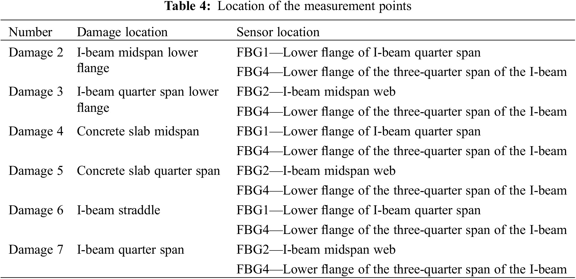
Four FBG strain sensors were placed on the composite beams at various positions to obtain strain signals. The specific locations of the sensors were the I-steel lower flange surface (FBG1, FBG4), the I-steel web surface (FBG2) and the lower surface of the concrete slab (FBG3) at the one-quarter and three-quarter spans of the composite beams. The specific location is shown in Fig. 9.

Figure 9: Strain measuring point layout diagram

3.6 Excitation Test

The excitation test obtained the strain signals when the composite beams were impacted at various positions. Specifically, steel balls of varying quality moved in free fall from different heights above the composite beam and fell in distinct positions on the composite beam to impact the different sizes of the composite beam. The weights of the steel balls were 500, 1000 and 1500 g, respectively. Fig. 10 shows the actual picture of the experiment. Before the excitation test, the composite beam was divided into 32 parts along the beam length and 6 parts along the beam width, forming 192 grids as different points on the steel ball. During the test, signal collection was interrupted when steel balls of the same quality were too high in height. Because the impact load was too large, the strain vibration signal of the beam exceeds the collection range of the sensor. However, if the height is too low and the impact load is too low, the vibration signal is not obvious, so the reasonable free fall height of the steel balls was in the range of 0.4~0.6 m.

Figure 10: Test images

4  Damage Identification

4.1 Strain–Time Domain Signals

In this test, 33,264 valid samples (strain time domain signals) were collected. Fig. 11 shows the strain time domain signal samples of the composite beam arbitrarily selected under different excitations. Fig. 11 shows that after the composite beam is stimulated by the steel ball, the strain vibration signal drops and continues for a period, but it is difficult to determine the damage state of the composite beam directly according to the strain time domain signal.

Figure 11: Time domain signal of strain in partially composite beams

4.2 Strain Signal Denoising and Time-Frequency Transformation via Wavelet Algorithms

In addition to the strain signal caused by steel ball excitation, the strain signal of a composite beam collected in a natural environment contains considerable noise, so it is necessary to reduce the noise in the strain signal collected in the time domain. In this paper, the Bayes algorithm described in Section 1 is used to decompose the signal, and five different wavelet basis functions, harr, sym2, sym4, db2 and db4, are selected for decomposition. The median function is subsequently used for filtering, after which all the subsignals are reconstructed. The strain time domain signals undenoised and denoised are shown in Fig. 12.

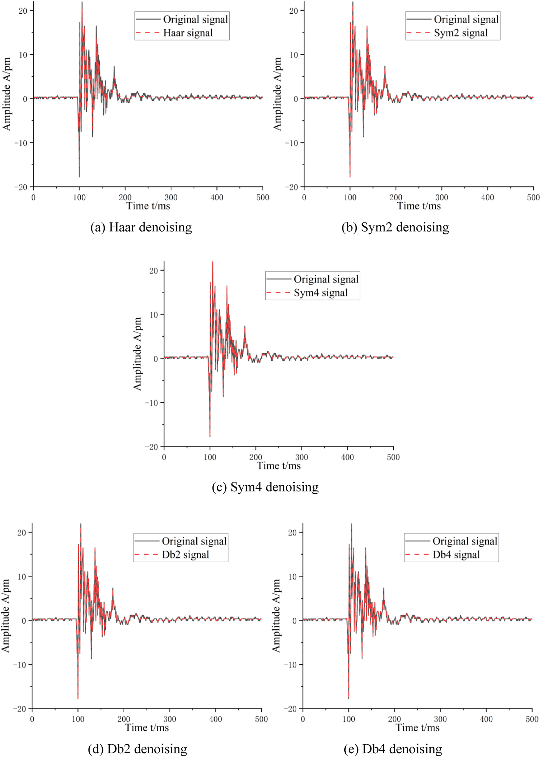
Figure 12: Comparison of the effects of the different denoising methods

The strain time signal after noise reduction is smoother than is the original signal, but it is still difficult to distinguish the damage category of the composite beam directly according to the strain time signal. The wavelet time-frequency transform is used to transform the strain time domain signal undenoised and denoised into two-dimensional time-frequency graphs, as shown in Fig. 13. The deep learning model is subsequently used to classify the two-dimensional time-frequency graphs.

Figure 13: Time-frequency diagram of the combined beam undenoising and denoising conditions

4.3 Build Data Set

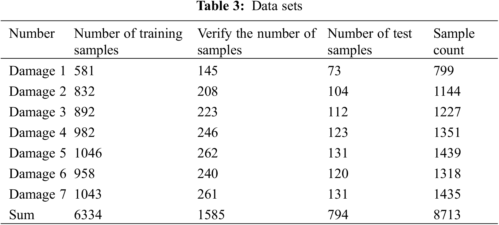
According to the above method, a total of 8713 strain time-frequency images of 6 kinds of damaged composite beams and undamaged composite beams were obtained; these images were randomly divided into a training set and a verification set, with a test set at a ratio of 8:2:1.

This study on addressing overfitting by implementing strategies such as hyperparameter tuning and regularization. Hyperparameters, including batch size, learning rate, and epochs, were meticulously calibrated through experimental validation to achieve a model configuration that effectively balances complexity and generalization. Additionally, regularization, for example, using MATLAB’s default parameter, was integrated into the training process to reduce weight dominance and encourage simpler models. The performance of the model was evaluated by monitoring training and validation curves. Moreover, the dataset was divided into training, validation, and test sets to ensure an unbiased evaluation. Overall, these approaches, encompassing hyperparameter tuning, regularization, curve analysis, and dataset partitioning, the study effectively addressed issues of both overfitting and underfitting. Meanwhile, to determine the optimal values for these hyperparameters, we utilized a combination of random search and manual adjustment. This approach allowed us to explore a wide range of hyperparameter values.

4.4 Model Training and Evaluation Metrics

Six deep learning models, namely, ResNet-18, ResNet-50, ResNet-101, InceptionV3, InceptionResNetV2 and MobileNetV2, were established. The batch size, learning rate, and epochs for each model were adjusted to optimize the model. During model training, the gdm optimization algorithm, ReLU activation function and cross-entropy loss function were used. The feature extraction process for deep learning models is illustrated in Fig. 14.

Figure 14: Example of the feature extraction process

Common performance evaluation metrics for deep learning models include accuracy and average accuracy. After the predictions from the model, correctly identified samples were termed true positives (TPs), while incorrectly recognized samples were considered false-negatives (FNs). If the model recognized the error class as correct, it was considered a false-positive (FP). The precision (P) is the ratio of correctly identified samples to the total samples classified in that category.

P=TPTP+FP (4)

The average precision, denoted as mP, is calculated by averaging the precision for each class (N is the total number of classes) in the validation set. A higher average precision indicates better model performance.

mP=∑PiN (5)

4.5 Identification Results and Analysis

To determine which wavelet basis function has the best denoising effect, the acquired strain signal is denoised according to the five wavelet basis functions mentioned in Section 3.2. Then, the wavelet time-frequency transform is used to transform the strain time domain signal denoised into two-dimensional time-frequency graphs, and MobileNetV2 and ResNet-50 are used to identify damage. The recognition results are shown in Table 3. The models in this study were subjected to five iterations, resulting in five distinct values. The mean of these five values represents the final mP value for the model within the given dataset.

Figs. 15 and 16 show that the data set training model using harr wavelet basis function to de-noise has smaller losse and faster convergence. Fig. 17 illustrates that the Haar wavelet basis function has the best denoising effect, and the mP values are increased by 7.59% and 1.18% compared with those of the undenoised dataset. However, in the prediction results of ResNet-50, when the sym2, sym4, db2 and db4 wavelet basis functions are used, the mP value is slightly lower than that of the undenoised dataset. This is because some signal features are like the noise components, and denoising may misjudge and eliminate some signal features. The feature extraction capability of the ResNet-50 network model is stronger than that of the MobileNetV2 network model, but the mP values of some features eliminated by denoising are lower.

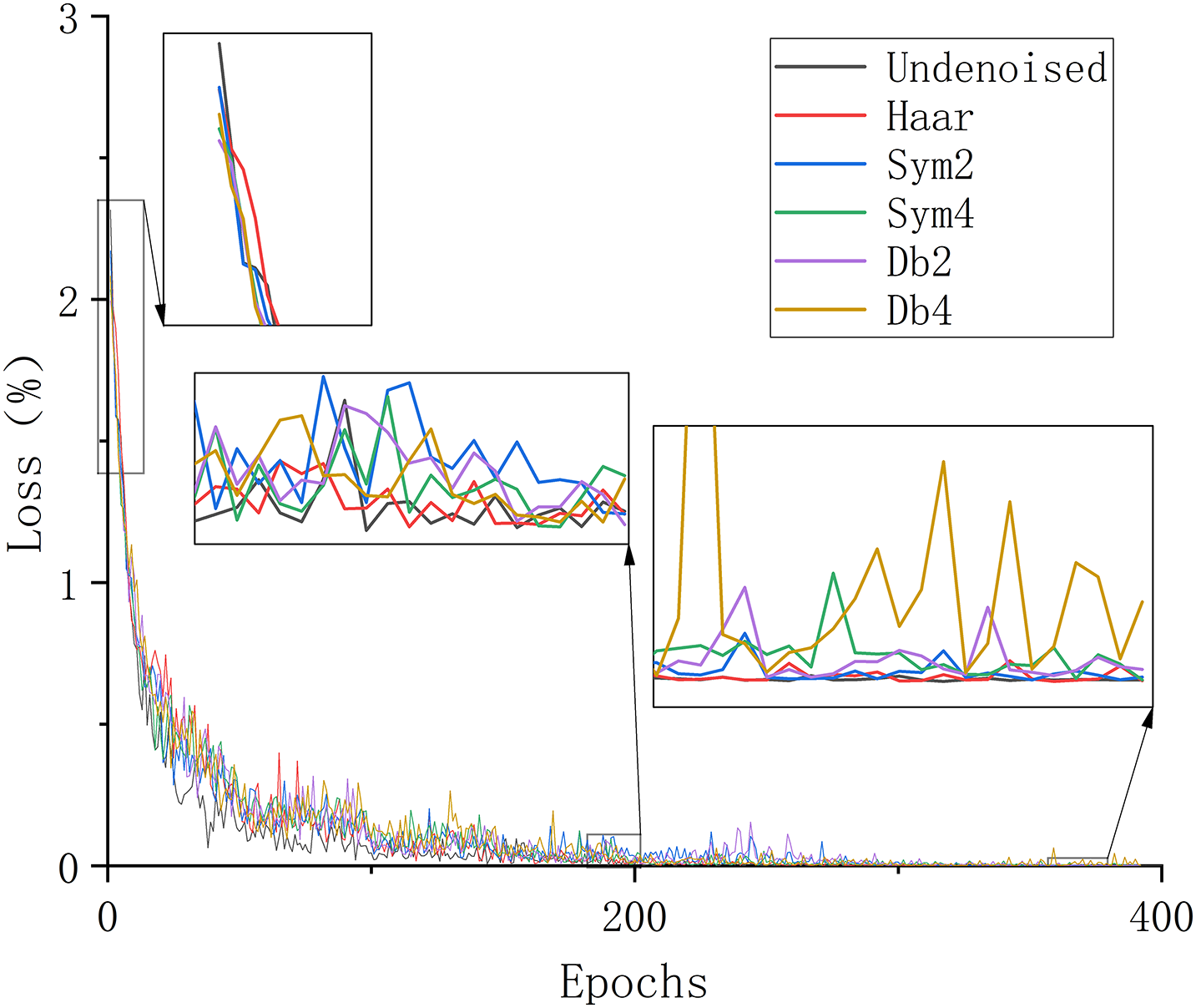
Figure 15: Comparison of loss across different denoising functions (ResNet-50)

Figure 16: Comparison of accuracy across different denoising functions (ResNet-50)

Figure 17: Comparison of the effects of denoising functions on the prediction results

Fig. 17 compares only the prediction results of the two deep learning models. In this section, the denoised training set is used to train six deep learning network models, ResNet-18, ResNet-50, ResNet-101, InceptionV3, InceptionResNetV2 and MobileNetV2, until the optimal model is obtained. The test set was subsequently evaluated, and each model was trained five times to obtain the average accuracy rate. The mP values of the undenoised and denoised samples are shown in Table 4 below.

Figs. 18 and 19 show that using the ResNet-50 model has smaller losses and faster convergence. Fig. 20 reveals that all six deep learning models established in this study accurately recognized the types and locations of damage sets for the composite beams with high accuracy. After denoising, the mP values of all six deep learning models improved. Specifically, the mP values for ResNet-18, ResNet-50, ResNet-101, InceptionV3, InceptionResNetV2 and MobileNetV2 were 96.54%, 97.91%, 97.5%, 96.73%, 95.97% and 95.99%, respectively.

Figure 18: Comparison of loss across different deep learning models

Figure 19: Comparison of accuracy across different deep learning models

Figure 20: Comparison of prediction results of different deep learning models

Specifically, MobileNetV2 showed a remarkable increase in mP of 7.59%. For the after-denoising test sets, the mP values in the predictions made by ResNet-50 were greater than those of the other models, with a 1.18% increase in mP values after denoising.

4.6 Influence of Sensor Location on Damage Identification Results

In this paper, four FBG sensors were used to collect the strain time domain signal of the composite beam. Some of the sensors were close to the damage location, but the damage location cannot be predicted in practical applications. To analyse its impact on the recognition results, the collected samples were screened in this section, and the samples collected by sensors far from the damage zone were evaluated. For example, the signals collected by sensors FBG1 (placed at the lower flange of one quarter of the I-span) and FBG4 (placed at the lower flange of three quarters of the I-span) were selected for the excitation test of the composite beam with damage 2 (middle of the I-span). Other damage type samples were screened in this way, as shown in Table 4.

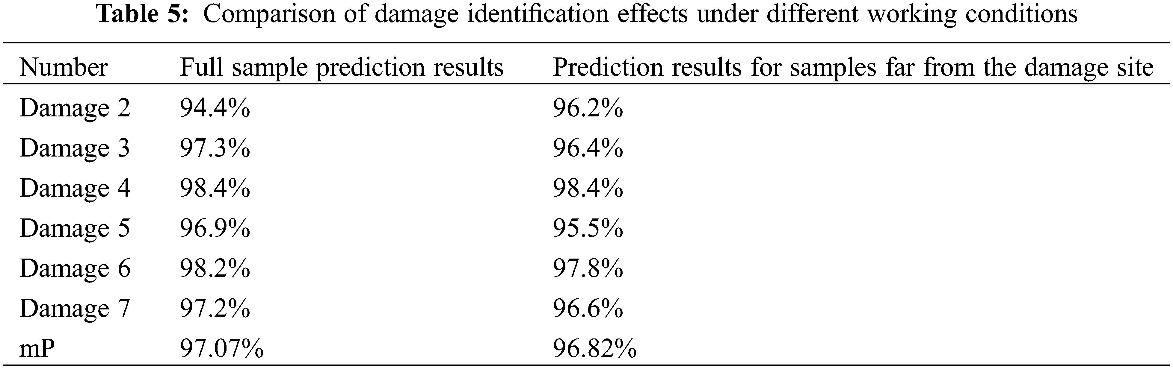
The data samples far from the damage location were input into the optimal depth residual network (ResNet-50) model obtained in the above section to obtain damage recognition and prediction results under various working conditions. The prediction accuracy is shown in Table 5. The mP value of the prediction for samples far from the damage location is 96.6%, and there is still a high accuracy rate. The signal collected by the sensor far from the damage site also contained damage information from the composite beam, and the depth residual network can be used to accurately extract these damage features. This section further verifies the reliability of this identification method.

5  Conclusions

In this paper, a new method was proposed for identifying damage in I-beam steel-concrete composite beams. Wavelet denoising and deep learning were used to identify composite beam damage. Fiber grating sensors were used to collect the strain time history signals of composite beams with different damage levels under different excitations. The two-dimensional time-frequency graph dataset was subsequently obtained via wavelet time-frequency transform. Multiple deep learning models were built to train and to predict the strain signals un-denoised and denoised; these predictions were used to classify and locate the damage in composite beams.

Following the experiments, the study yields the following conclusions:

1) The low-temperature-sensitive quasi-distributed long-distance fiber grating strain sensor used in this experiment has the advantages of low temperature strain, easy layout, high sensitivity, high resolution, and strong anti-interference ability and can be used to successfully collect the strain signal during the whole excitation test.

2) In the denoising phase of this study, the method used showed an improvement in model test accuracy compared to other methods employing wavelet basis function denoising, with the least improvement being 1.18% and the greatest being 4.45%. Furthermore, during the model training phase of this study, the approach demonstrated a discernible improvement in test accuracy over other models, with increases varying from 0.41% at the minimum to 1.94% at the maximum.

3) Even strain–time domain signals collected from sensors positioned further from the damage location in this experiment encompass information regarding the damage in the composite beams. The deep learning models designed for this experiment can accurately extract these damage characteristics.

Acknowledgement: None.

Funding Statement: The authors received no specific funding for this study.

Author Contributions: The authors confirm contribution to the paper as follows: study conception and design: Caiping Huang, Chengpeng Zhang; data collection: Chengpeng Zhang; analysis and interpretation of results: Junfeng Shi; draft manuscript preparation: Caiping Huang, Chengpeng Zhang. All authors reviewed the results and approved the final version of the manuscript.

Availability of Data and Materials: All data generated or analysed during this study are included in this published article.

Conflicts of Interest: The authors declare that they have no conflicts of interest to report regarding the present study.

References

1. Jun, S. C., Lee, C. H., Han, K. H., Kim, J. W. (2018). Flexural behavior of high-strength steel hybrid composite beams. Journal of Constructional Steel Research, 149, 269–281. https://doi.org/10.1016/j.jcsr.2018.07.020 [Google Scholar] [CrossRef]

2. Wen, Q., Hua, X. G., Chen, Z. Q., Guo, J. M., Niu, H. W. (2017). Modal parameter identification of a long-span footbridge by forced vibration experiments. Advances in Structural Engineering, 20(5), 661–673. https://doi.org/10.1177/1369433217698322 [Google Scholar] [CrossRef]

3. Baghlani, A., Baghlani, A. (2021). Enhancing the curvature mode shape method for structural damage severity estimation by means of the distributed genetic algorithm. Engineering Optimization, 53(4), 683–701. https://doi.org/10.1080/0305215X.2020.1746294 [Google Scholar] [CrossRef]

4. He, R., Zhu, Y. F., He, W., Chen, H. (2018). Structural damage recognition based on perturbations of curvature mode shape and frequency. Acta Mechanica Solida Sinica, 31(6), 794–803. https://doi.org/10.1007/s10338-018-0058-y [Google Scholar] [CrossRef]

5. Rubio, L., Fernández-Sáez, J., Morassi, A. (2018). Identification of an open crack in a beam with variable profile by two resonant frequencies. Journal of Vibration and Control, 24(5), 839–859. https://doi.org/10.1177/1077546316671483 [Google Scholar] [CrossRef]

6. Cho, D. S., Kim, J. H., Choi, T. M., Kim, B. H., Vladimir, N. (2018). Free and forced vibration analysis of arbitrarily supported rectangular plate systems with attachments and openings. Engineering Structures, 171, 1036–1046. https://doi.org/10.1016/j.engstruct.2017.12.032 [Google Scholar] [CrossRef]

7. Ciambella, J., Pau, A., Vestroni, F. (2019). Modal curvature-based damage localization in weakly damaged continuous beams. Mechanical Systems and Signal Processing, 121, 171–182. https://doi.org/10.1016/j.ymssp.2018.11.012 [Google Scholar] [CrossRef]

8. Rhif, M., Ben Abbes, A., Farah, I. R., Martínez, B., Sang, Y. F. (2019). Wavelet transform application for/in non-stationary time-series analysis: A review. Applied Sciences, 9(7), 1345. https://doi.org/10.3390/app9071345 [Google Scholar] [CrossRef]

9. Ghasemi-Ghalebahman, A., Ashory, M. R., Kokabi, M. J. (2018). A proper lifting scheme wavelet transform for vibration-based damage identification in composite laminates. Journal of Thermoplastic Composite Materials, 31(5), 668–688. https://doi.org/10.1177/0892705717718239 [Google Scholar] [CrossRef]

10. Ashory, M. R., Ghasemi-Ghalebahman, A., Kokabi, M. J. (2018). Damage identification in composite laminates using a hybrid method with wavelet transform and finite element model updating. Proceedings of the Institution of Mechanical Engineers, Part C: Journal of Mechanical Engineering Science, 232(5), 815–827. https://doi.org/10.1177/0954406217692844 [Google Scholar] [CrossRef]

11. Ma, Q. Y., Solís, M., Galvín, P. (2021). Wavelet analysis of static deflections for multiple damage identification in beams. Mechanical Systems and Signal Processing, 147, 107103. https://doi.org/10.1016/j.ymssp.2020.107103 [Google Scholar] [CrossRef]

12. Shi, L. Z., Cheng, B., Li, D. R., Xiang, S., Liu, T. C. (2023). A CNN-based lamb wave processing model for field monitoring of fatigue cracks in orthotropic steel bridge decks. Mechanical Systems and Signal Processing, 147, 105146. https://doi.org/10.1016/j.ymssp.2020.107103 [Google Scholar] [CrossRef]

13. Zhuo, D. B., Cao, H. (2022). Damage identification of bolt connection in steel truss structures by using sound signals. Structural Health Monitoring, 21(2), 501–517. https://doi.org/10.1177/14759217211004823 [Google Scholar] [CrossRef]

14. Huynh, T. C. (2021). Vision-based autonomous bolt-looseness detection method for splice connections: Design, lab-scale evaluation, and field application. Automation in Construction, 124, 103591. https://doi.org/10.1016/j.autcon.2021.103591 [Google Scholar] [CrossRef]

15. Cha, Y. J., Choi, W., Büyüköztürk, O. (2017). Deep learning-based crack damage detection using convolutional neural networks. Computer-Aided Civil and Infrastructure Engineering, 32(5), 361–378. https://doi.org/10.1111/mice.12263 [Google Scholar] [CrossRef]

16. Zhu, J. S., Zhang, C., Qi, H. D., Lu, Z. Y. (2020). Vision-based defects detection for bridges using transfer learning and convolutional neural networks. Structure and Infrastructure Engineering, 16(7), 1037–1049. https://doi.org/10.1080/15732479.2019.1680709 [Google Scholar] [CrossRef]

17. Huang, C., Zhai, K. K., Xie, X., Tan, J. (2021). Deep residual network training for reinforced concrete defects intelligent classifier. European Journal of Environmental and Civil Engineering, 26(15), 7540–7552. https://doi.org/10.1080/19648189.2021.2003250 [Google Scholar] [CrossRef]

18. Nie, L., Wang, W., Deng, L., He, W. (2022). ANN and LEFM-based fatigue reliability analysis and truck weight limits of steel bridges after crack detection. Sensors, 22(4), 1580. https://doi.org/10.3390/s22041580 [Google Scholar] [PubMed] [CrossRef]

19. Lu, N. W., Noori, M., Liu, Y. (2017). Fatigue reliability assessment of welded steel bridge decks under stochastic truck loads via machine learning. Journal of Bridge Engineering, 22(1), 04016105. https://doi.org/10.1061/(ASCE)BE.1943-5592.0000982 [Google Scholar] [CrossRef]

20. Sun, X. T., Xin, Y., Wang, Z. C., Yuan, M. G., Chen, H. (2022). Damage detection of steel truss bridges based on gaussian bayesian networks. Buildings, 12(9), 1463. https://doi.org/10.3390/buildings12091463 [Google Scholar] [CrossRef]

21. Luo, H., Li, C. B., Wu, M. Q., Cai, L. M. (2023). An enhanced lightweight network for road damage detection based on deep learning. Electronics, 12(12), 2583. https://doi.org/10.3390/electronics12122583 [Google Scholar] [CrossRef]

22. Guo, A. P., Jiang, A. J., Lin, J., Li, X. X. (2020). Data mining algorithms for bridge health monitoring: Kohonen clustering and LSTM prediction approaches. Journal of Supercomputing, 76(2), 932–947. https://doi.org/10.1007/s11227-019-03045-8 [Google Scholar] [CrossRef]

23. Li, C. L., Tang, J. G., Cheng, C., Cai, L. B., Yang, M. H. (2021). FBG arrays for quasi-distributed sensing: A review. Photonic Sensors, 11(1), 91–108. https://doi.org/10.1007/s13320-021-0615-8 [Google Scholar] [CrossRef]

24. Jinachandran, S., Rajan, G. (2021). Fibre bragg grating based acoustic emission measurement system for structural health monitoring applications. Materials, 14(4), 897. https://doi.org/10.3390/ma14040897 [Google Scholar] [PubMed] [CrossRef]

25. Geng, X. Y., Lu, S. Z., Jiang, M. S., Sui, Q., Lv, S. et al. (2018). Research on FBG-based CFRP structural damage identification using BP neural network. Photonic Sensors, 8(2), 168–175. https://doi.org/10.1007/s13320-018-0466-0 [Google Scholar] [CrossRef]

26. Karatas, C., Degerliyurt, B., Yaman, Y., Sahin, M. (2020). Fibre Bragg grating sensor applications for structural health monitoring. Aircraft Engineering and Aerospace Technology, 92(3), 355–367. https://doi.org/10.1108/AEAT-11-2017-0255 [Google Scholar] [CrossRef]