Damage Diagnosis of Bleacher Based on an Enhanced Convolutional Neural Network with Training Interference

1  Introduction

With the development of the construction industry, bleachers have been widely used in gymnasiums, schools, performances, and many other areas. The use of bleachers involves the safety of people, and it is a significant task for researchers to diagnose the structural damage of the bleacher and evaluate the overall risk. Traditional methods of periodic inspection are expensive and ineffective due to the structure of the bleacher is complex and various factors that can cause damage to the bleacher, such as personnel movement and environmental corrosion. Therefore, researchers have proposed many new fault diagnosis methods to make structural health monitoring (SHM) techniques better developed [1–5], this is particularly important for predicting and diagnosing bleacher damage.

The data-driven approach is commonly employed for diagnosing bleacher damage and assessing its overall performance, which mainly includes data acquisition, modeling, data analysis, and data feedback. When it comes to diagnosing bleacher damage using a data-driven approach, it entails analyzing the operational state of the bleacher based on the collected data. The traditional damage diagnosis methods based on vibration data are usually time−domain analysis, frequency−domain analysis, and time−frequency analysis [6–8]. In order to better represent the local characteristics of vibration data, time−frequency analysis methods such as cepstrum analysis [9], envelope spectrum analysis [10], wavelet transform [11], local mean decomposition [12], and short−time Fourier transform [13] are usually used. Luo et al. proposed a fault diagnosis method based on wavelet packet and cepstrum analysis and applied it to the gearbox fault diagnosis of wind turbine [14]. Chen et al. proposed an integrated fault diagnosis method based on resonance sparse signal decomposition and wavelet transform, this method solved the problem of low diagnosis accuracy of rolling bearing under strong noise interference [15]. Bayat et al. have made significant contributions in various areas of structural engineering and dynamics. Their research includes the utilization of Added Damping and Stiffness (ADAS) devices for energy dissipation in building structures subjected to seismic ground motions. They have also applied He’s variational approach method to study large-amplitude free vibration in mechanical systems with linear and nonlinear springs. Additionally, their work involves addressing nonlinear oscillators with discontinuities, demonstrating the effectiveness of their methods for a wide range of vibration amplitudes. Furthermore, they have proposed an innovative algorithm for seismic damage detection in bridge piers, utilizing analytical models and the Power Spectral Density function for dynamic characterization, with a focus on output-only methods that eliminate the need for excitation force measurements and numerical models [16–19]. In the field of structural damage identification and dynamic model updating, Sehgal and his colleagues have introduced innovative methodologies to accurately assess structural damage and damping effects. Their contributions include a two-stage damped updating method that employs multi-objective optimization techniques for precise damage and damping parameter identification. Additionally, they applied structural dynamic model updating to evaluate the extent of damage at six different locations on a damaged cantilever beam structure. They further developed a novel dynamic model updating technique that incorporates response surface models and Derringer’s function approach, enabling multi-objective optimization for updating both elastic parameters and damping constants. Finally, their research presented the application of a weighted model updating method based on Derringer’s functions for enhanced damage detection performance [20–23]. Dinh-Cong et al. introduced an optimization-based model updating technique using Chaos Game Optimization (CGO), capable of addressing incomplete noisy measurements and temperature variations, demonstrating exceptional performance in locating and quantifying damage in metallic structures [24]. In the face of complex and changeable environment, the traditional damage diagnosis methods will become difficult to extract features of vibration data, and the performance of damage diagnosis will not become ideal due to the difference between data probability distribution.

With the development of deep learning, it has been widely used in image recognition [25–28], speech recognition [29–33], driverless [34,35], and other fields. Typical deep learning models include stack auto−encoder (SAE) [36], recurrent neural networks (RNN) [37], generative adversarial networks (GAN) [38], and convolutional neural networks (CNN) [39]. Wang et al. used stacking autoencoders to train deep networks and solved the problem of poor correlation between deep features and fault types [40]. Graves et al. obtained high accuracy in TIMIT speech recognition by using deep cycle neural networks and appropriate regularization training [41]. Zhang et al. proposed an adjunctive neural network based on an attention mechanism that can realize remote modeling of image generation tasks and generate corresponding detailed information by using the prompts of all feature positions [42]. Gullu et al. used artificial intelligence techniques such as radial basis neural network (RBNN) [43], generalized regression neural network [44], adaptive neuro−fuzzy inference system [45], and multilayer perceptron [46] to predict the unconfined compressive strength of silty soil under different freeze−thaw cycles; experimental results show that the prediction accuracy of the artificial intelligence technology is higher than that of the nonlinear regression method, and RBNN has the best prediction effect [47].

Among the above multiple deep learning models, CNN has powerful feature extraction and information fusion capabilities, which has provided new research ideas for SHM and damage diagnosis [48,49]. Lei et al. input the collected vibration signal directly into the model and used an unsupervised two−layer neural network structure to classify the data [50]. Jing et al. proposed a method that can learn different features adaptively, which achieved high diagnosis accuracy of gearbox dataset provided by prognostics and health management (PHM) [51]. Wen et al. converted the original vibration signal into two−dimensional grayscale pictures and input them into the LeNet−5 model [52] for training, which significantly improved diagnosis accuracy compared with the traditional methods [53]. Zhou et al. also used the original vibration signal and performed fault diagnosis of rotating machinery based on the classical AlexNet [54] structure [55]. Levent et al. proposed a one−dimensional convolutional neural network (1DCNN) model based on the vibration signal for fault diagnosis of rolling bearings [56]. Abdeljaber et al. used 1DCNN to diagnosis the fault of the bleacher model and realized real−time SHM of the bleacher [57]. However, because the used 1DCNN model only has two convolutional layers and two fully connected layers, and the convolutional kernel size of each layer is the same, the generalization ability of the model is unsatisfied, and the accuracy and anti−noise ability are relatively low. In order to improve the accuracy and anti−noise ability of CNN, Zhang et al. proposed a CNN model named convolutional neural networks with training interference (TICNN) and applied it to the fault diagnosis of bearings with satisfactory results [58].

Although the diagnosis accuracy of the TICNN model in bearing fault diagnosis has been close to 100%, there are still some challenges when applying it to bleacher damage diagnosis. (1) The existence of its deep structure leads to a large amount of computation in the training process of the model, which hinders real−time diagnosis of bleacher issues. (2) Due to the similarity of damage data in the adjacent locations of the bleacher, the classification accuracy is reduced, and the final result is not ideal. In order to improve the accuracy and anti−noise ability of the damage diagnosis of the bleacher, this paper improved TICNN and proposed an enhanced TICNN model named ETICNN. The proposed new model changed the data input length of the original model, and optimized a series of structural parameters of the original model, such as the convolutional layer, pooling layer, and fully connected layer, so as to reduce the calculation amount and total number of parameters of the original model, and avoided overfitting of the model. The contribution of this paper is to propose an ETICNN model with high accuracy and strong anti−interference ability and apply this model to bleacher damage diagnosis.

2  Structure and Data Source of Bleacher

This paper took the bleacher simulator built by Qatar University (QU) as the experimental object, and the experimental data in this paper also came from the open data set of QU. The 3D model of QU’s bleacher simulator and the specific location of each acceleration sensor are shown in Fig. 1 [57]. It can be seen from the figure that the overall size of the bleacher simulator built by QU is about 4.2 m × 4.2 m, it consists of 8 main beams, 25 filled beams, and 4 columns. Different damages of the bleacher can be obtained by loosening the bolts at different joints. The bleacher simulator can accommodate 30 spectators, and 30 acceleration sensors were installed at the location shown in Fig. 1 to collect the vibration data of the bleacher. These accelerometers consist of 27 PCB model 393B04 units and 3 B&K model 8344 units. To attach these accelerometers to the steel structure, magnetic mounting plates of PCB model 080A121 were used. Additionally, a modal shaker (Model 2100E11) was employed to induce vibration in the structure. The vibration signal was delivered to the shaker through a SmartAmp 2100E21−400 power amplifier. Two 16−channel data acquisition devices were utilized to generate input signals for the shaker and collect acceleration output signals. It can test the performance of multiple damage detection methods by collecting data under different structural configurations during the experiment. The number of the sensor is the same as the number of the location where it is installed. In this paper, the vibration data collected by sensors numbered 1−30 are used as training samples to study the damage diagnosis of the bleacher.

Figure 1: 3D model of QU’s bleacher simulator

3  Damage Diagnosis of Bleacher

3.1 Damage Diagnosis Principle

The damage diagnosis method for the bleacher based on CNN proposed in this paper can determine the damage location through vibration data. It uses CNN to independently train data samples from 30 acceleration sensors, and obtains 30 CNN models. The overall damage diagnosis principle of the bleacher includes data acquisition, data preprocessing, CNN model training, and damage diagnosis results. Data acquisition is to collect the vibration signals. Data preprocessing is mainly used to obtain enough input data that can be accepted by CNN model. CNN model training is mainly used for feature extraction and classification, and different features are used to distinguish the damage of the bleacher, and the specific damage diagnosis results can be obtained.

3.2 Damage Diagnosis Process

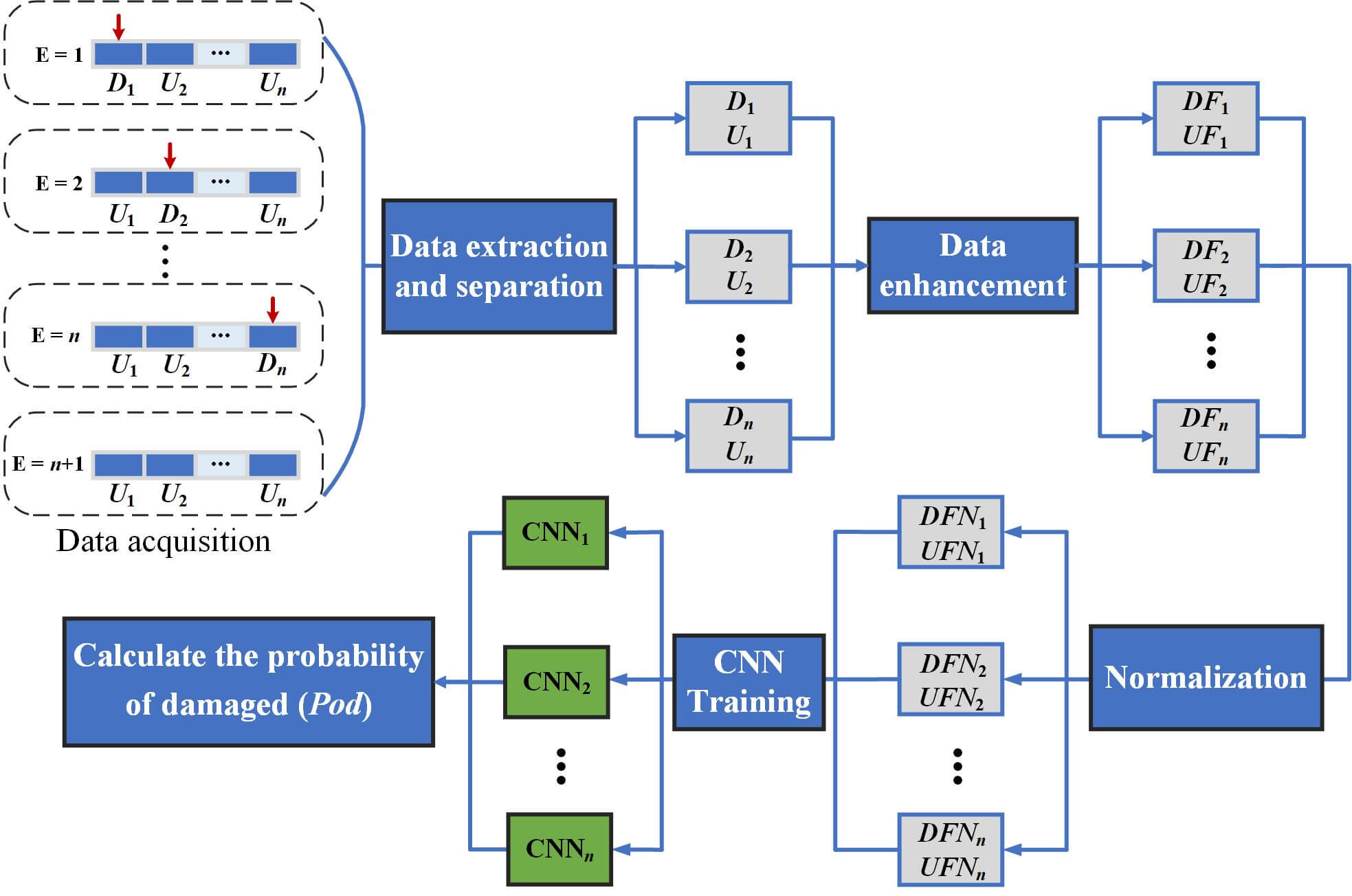
The damage diagnosis process is shown in Fig. 2. It includes data acquisition and preprocessing, CNN model training, and damage probability calculation.

Figure 2: Damage diagnosis process

(1) Data acquisition and preprocessing

Data acquisition and preprocessing include data acquisition, data extraction and separation, data enhancement and data normalization.

a. Data acquisition, extraction and separation

Assuming n locations to be detected during the experiment, the bleacher needs to be tested n + 1 times. The first experiment is to destroy the structure at the location numbered 1. The n experiment is to destroy the structure at the location numbered n, and then collect the vibration signal. The n + 1 experiment is to collect the vibration signal when the bleacher is undamaged. The data collected by all acceleration sensors under the condition of damaged were denoted as D, and those collected under the condition of undamaged were denoted as U. Then the vibration signals were extracted and separated to make a dataset. It can be written as follows:

D=[D1,D2,⋯,Dn] (1)

U=[U1,U2,⋯,Un] (2)

b. Data enhancement

The number of direct slices of the data collected during the experiment is insignificant. In order to avoid the problem of model overfitting caused by too small dataset, data enhancement methods are used to obtain more samples. Data enhancement is realized by using sliding window overlapping sampling. There is an overlap between the previous signal and the latter signal of the generated dataset. For example, for a signal with K points, N samples can be obtained by using sliding window overlapping sampling with a window size of W and step of S.

N=K−WS+1 (3)

The K of the collected dataset published by QU is about 260,000. If W is 1024 and S is 128, the total number of data samples N is 2040. DF and UF were used to represent damaged and undamaged data after data enhancement, respectively.

DF=[DF1,DF2,⋯,DFn] (4)

UF=[UF1,UF2,⋯,UFn] (5)

c. Data normalization

In deep learning, different feature vectors usually have different dimensions, which will affect the results of data analysis. In order to solve the comparability between data index, data should usually be normalized. Data normalization can summarize the statistical distribution of uniform samples. The objective function of normalized data will be smoother during the training process, which can speed up the training, avoid the problems of gradient disappearance and gradient explosion, and ensure the network training more stable. The data in each case of DF and UF (4080 groups in total) were normalized between [−1, 1], and DFN and UFN were used to represent the data after normalization and disorder, respectively.

DFN=[DFN1,DFN2,⋯,DFNn] (6)

UFN=[UFN1,UFN2,⋯,UFNn] (7)

(2) CNN model training

The normalized data can be used to train the CNN at each location separately. Firstly, the data was divided into two parts: the training set and validation set. The total number of training samples corresponding to each CNN is 4080. 70% of the data was used as the training set, and the remaining 30% was used as the validation set. Then the divided data was input into the model for training, and the trained CNN model was saved for testing. The function of the training set was to constantly update the model parameters through forward propagation and back propagation to achieve the best effect of the model. The function of the validation set was to conveniently observe the performance of the model during the training process by calculating performance evaluation indicators such as the accuracy. In the training process, Adam optimization algorithm was used to ensure that the model can achieve the best performance. The data of the test set was new data that was not involved in the training process. The number of samples in the test set was the same as the number of samples in the training set, and it was necessary to randomly disrupt the order, and then input it into the saved CNN model to get the prediction results.

(3) Calculate the actual damage probability

The n−th CNN model saved by training can be used to predict and classify the damage at the n−th location. In this paper, the actual damage probability (Pod) was used to express the damage degree of a certain location. The larger the value is, the more serious the damage is. The calculation equation of the Pod can be written as follows:

Pod=DNTN (8)

where DN represents the number of damaged samples predicted by the model, TN represents the total number of test set samples.

4  Structure of ETICNN Model

In order to improve the accuracy and anti−noise ability of the damage diagnosis of the bleacher, this paper improved TICNN and proposed an enhanced TICNN model named ETICNN. The detailed structures of TICNN model and ETICNN model are shown in Fig. 3.

Figure 3: Structures of TICNN model and ETICNN model

In convolutional neural network, the size of the receptive field affects the feature extraction ability of the convolutional layer. When the receptive field is large, the collected feature information tends to be more macroscopic, and when the receptive field is small, the feature information tends to be more local. Under the same experimental conditions, the influence of kernel size and stride of the first convolutional layer on accuracy and loss was studied, and the appropriate kernel size and stride were selected. The results are shown in the Table 1. As can be seen from the table, when the kernel size is 128 and the stride is 8, the model has the highest accuracy and lower loss value. At this time, Train−Acc is 98.8%, Valid−Acc is 98.6%, Train−Loss is 0.068, Valid−Loss is 0.051.

It can be seen from Fig. 3 that after the model was adjusted, the convolutional kernel size of the first convolutional layer was set to 128 × 1, and the number of convolution kernels was set to 16, and Dropout was added after the first convolutional layer to suppress the overfitting phenomenon of the model. The convolutional kernel size in the second part was set to 64 × 1, the number of convolution kernels was set to 32, and the stride was set to 4. The convolutional kernel size in the third part was set to 32 × 1, the number of convolution kernels was set to 64, and the stride was set to 2. Through the intermediate transition part, the overall receptive field has been increased, which can avoid the direct use of small convolution kernels in the early stage to extract the smaller receptive field. The convolutional kernel size of the remaining convolutional layers was set to 4 × 1, the number of convolution kernels was gradually increased to 256, and the stride was still set to 1.

It can be also seen from Fig. 3 that after each convolutional layer of the model, the max pooling layer and the BN layer were added. The distribution of data can be consistent through BN, thus making the model more stable during training. At the end of the model, the global average pooling layer was used instead of the fully connected layer. The global average pooling layer is an excellent structural choice for establishing the relationship between the feature map and the category. It sums the overall spatial information, and the spatial transformation of the input features is more stable. In addition, it does not require parameter optimization and can avoid the occurrence of overfitting.

5  Experiments

The contents of the experiments include damage diagnosis experiment phase I, damage diagnosis experiment phase II, ablation experiment, comparative experiment of diagnosis accuracy, and comparative experiment of anti−noise ability. In damage diagnosis experiment phase I, a binary classification method was used to train the neural network model of each location to ensure the diagnosis accuracy of the ETICNN of each location, so as to accurately distinguish between damaged and undamaged cases. The damage diagnosis experiment phase II was mainly conducted by using the same neural network model for multi−classification training. The purpose of multi−classification training is to test the classification and generalization ability of the network model under different conditions to determine the damage location of the bleacher. Due to the complexity of the damage case and the large number of damage locations involved in the experiment, the collected vibration data is huge. Therefore, only the data of sensors numbered 1−10 were selected as the research object in the damage diagnosis experiment phase II. For these 10 damage locations, the convolutional neural network was used for multi−classification training to identify the damage locations and test the generalization ability of the network model. The purpose of the ablation experiment is to prove the rationality of the model improvement and the impact of each part of the model on the performance. The comparative experiment of diagnosis accuracy and comparative experiment of anti−noise ability mainly compare the diagnosis ability between different models. The deep learning framework for these experiments is based on Tensorflow version 2.3.1, and the computer is a laptop with Core i5−7300HQ and NVIDIA GeForce GTX 1050 Ti GPU.

5.1 Damage Diagnosis Experiment Phase I

In the damage diagnosis experiment phase I, firstly, it is necessary to train the data collected by each sensor to obtain the ETICNN model of the corresponding location. The diagnosis effect of each ETICNN model was ensured through a series of analyses on the accuracy and confusion matrix of the training results. Then, the unknown data collected at each location were input into the corresponding ETICNN model to determine whether each location is damaged, so as to determine the specific damage location.

(1) Analysis of training results

There are 30 locations for damage diagnosis, so 30 training results have been obtained. For convenience, this paper took the training results of the data collected by the sensor numbered 5 (location 5) as an example to illustrate the performance of the ETICNN model. The accuracy and Loss at location 5 is shown in Fig. 4.

Figure 4: Accuracy and loss at location 5

As can be seen from Fig. 4, when the training epoch reaches 5, the amplitude change of accuracy and Loss curves begin to stabilize. When the training epoch reaches 25, the Loss is close to 10−3, and the accuracy is close to 100%. When the training epoch reaches 30, the accuracy curves and the Loss curves of the training set and the validation set are nearly coincident. This shows that the ETICNN model has fast convergence speed and high accuracy, and can be used to achieve accurate damage diagnosis of the bleacher.

(2) Confusion matrix analysis

In deep learning, the confusion matrix, also known as the error matrix, is used to summarize the results of a classifier. The recall and accuracy of the neural network can be obtained by calculating the data in the confusion matrix, which can help analyze the specific situation of each class and observe which class is not easily distinguishable between the actual class and the predicted class. The confusion matrix obtained by training data collected by the sensor numbered 5 is also used as an example; it is shown in Fig. 5.

Figure 5: Confusion matrix at location 5

As can be seen from Fig. 5, when the training epoch is 3, the accuracy is 88.5% and recall is 77%. When the training epoch is 30, the accuracy is 100% and the recall is also 100%. These results show that when ETICNN model is used to diagnose the damage location of the bleacher, it only needs 30 training epochs to reach a higher accuracy, which again proves that the ETICNN model has a faster convergence speed and higher accuracy.

(3) Diagnosis of specific damage location

In order to test the effectiveness of the trained ETICNN model in the actual process, in this paper, firstly, different locations of the bleacher were damaged under various conditions, and then the results were carried out by using the ETICNN model. When conducting damage diagnosis for different locations of the bleacher, this paper first used the new data not participating training as the test set, and input it into the model for diagnosis, and then calculated the probability of damage (Pod) of each location to determine whether the location is damaged. In the experiment, six kinds of damage cases were analyzed for the structure at locations 1−10.

In addition, these six kinds of damage cases can be divided into three categories. 1). Single location damage cases (only one location of the structure was damaged, the structure at locations 2, 5, and 9 was damaged separately, and other locations were intact, a total of 3 damage cases). 2). Two locations damage cases (at the same time, the structures at two locations were damaged; the structures at locations 1 and 6 were damaged at the same time; the structures at locations 4 and 7 were damaged at the same time; a total of two damage cases). 3). The structures at all locations were undamaged (one damage case). The damage diagnosis results are shown in Fig. 6.

Figure 6: Pod at specific locations

As can be seen from Fig. 6, the ETICNN model performs well in various structural damage cases. In the case of single location damage, the Pod at the specific damage location reaches as high as 99%, while the Pod of other undamaged locations is less than 20%. In the case of two locations damage, the damage probability is greater than 90%, and the probability of undamaged locations is less than 20%. In the undamaged case, the damage probability at all 10 locations is relatively low, around 15%. The experiment results have a high degree of distinction, and the specific damage location can be accurately determined by the peak in the figure. It can be seen from the training and test results of the damage location diagnosis of the bleacher that the ETICNN model can achieve ideal results. It can accurately diagnose whether the structure of the bleacher at a specific location is damaged.

5.2 Damage Diagnosis Experiment Phase II

The damage diagnosis experiment phase II is mainly to carry out multi−classification identification for structural damage at locations 1−10. That is to say, the structures at 10 locations are destroyed separately, and then the neural network model is used for classification and identification to obtain 10 different damaged conditions. The purpose of multi−classification training is to distinguish specific damage cases in the preset fault conditions quickly and to test the generalization ability of the model for other situations.

(1) Analysis of training results

The training results of the damage diagnosis experiment phase II are shown in Fig. 7 (a. the results when training epoch is 30; b. the results when training epoch is 100). As seen from the figure, when training epoch reaches 30, accuracy curves and Loss curves become smooth. The accuracy of the validation set and the training set are both over 98%. However, at this time, the target function value (Loss) of the training set is still considerable, the Loss of the validation set is about 0.05, and it has yet to reach the ideal value. When the training epoch reaches 100, the Loss of the training set drops to around 0.05, which is half of the value when the training epoch is 30; the Loss of the validation set fluctuates around 0.01, which is one−fifth of the value when the training epoch is 30. In general, for 10 categories, the ETICNN model has fast convergence speed and high accuracy, and can be used to achieve accurate diagnosis of damage conditions.

Figure 7: Training results of locations 1−10

(2) Confusion matrix analysis

The confusion matrix has been briefly introduced in previous section, and the analysis of the confusion matrix has been carried out under the training epoch is equal to 3, 30, and 100, respectively, and the results are shown in Fig. 8. It can be seen from the figure that the results are not ideal when the training epoch is 3. In comparison, the accuracy can reach 98.8% when the training epoch is 30, and the accuracy reaches 99.7% when the training epoch is 100, which shows that the accuracy and recall of the model have increased after multiple training. In addition, from the confusion matrix, it can clearly distinguish which location of the network model may have a deviation in the diagnosis results, and solving the deviation problem can effectively help the optimization of the network model in the follow−up work.

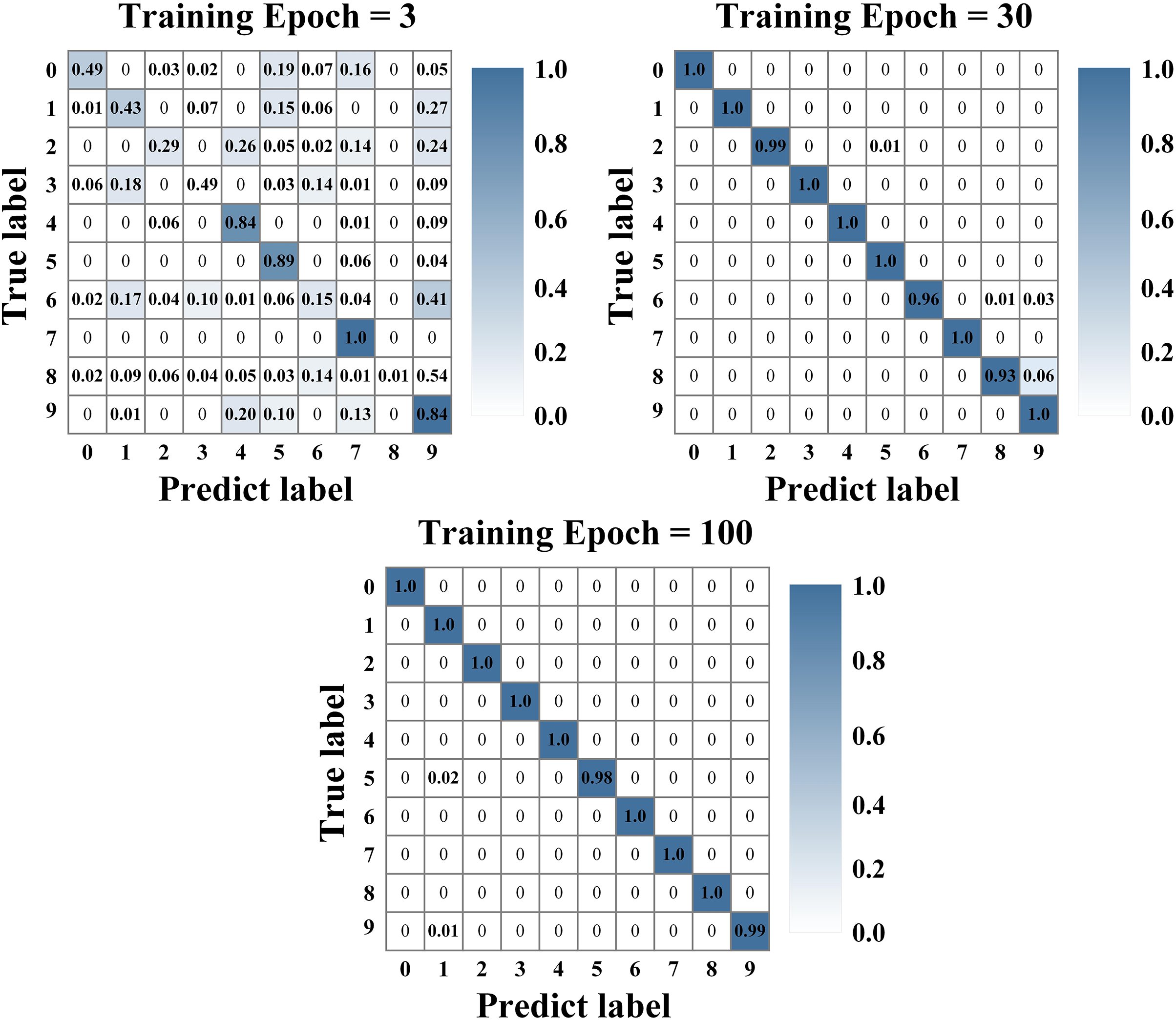
Figure 8: Confusion matrix of train dataset

(3) Test result analysis

The test process for damage diagnosis experiment phase II is to first save the weights of the trained network model (training epoch = 100), then input the new test dataset that has not been involved in the training into the saved model in a randomized order, and then view the final classification results through the confusion matrix. The confusion matrix results of the test dataset are shown in Fig. 9. In the experiment, locations 1−10 correspond to labels 0−9 in the figure, and the values of 10 cases are all 1.0. According to the calculation of the data in the figure that the accuracy of ETICNN is 100% in the test dataset and the recall is also 100%, this shows that ETICNN model has strong classification and recognition ability.

Figure 9: Confusion matrix of test dataset

5.3 Ablation Experiment

In order to study the effects of each part on the model, the experiment used the ETICNN (Normal), ETICNN without Dropout (NO−Dropout), ETICNN without BN (NO−BN), and ETICNN without global average pooling layer (NO−GAP) for comparison. Because the results of damage location diagnosis experiment are single, so the damage diagnosis experiment phase II was selected as the object for ablation experiment. In ablation experiment, the above four models were trained 10 epochs under the same condition, and the results are shown in Fig. 10. As can be seen from the figure, when the ETICNN model was used, the curves start to flatten after 3 epochs; the Loss of the validation set of NO−Dropout model fluctuates greatly during the training process; the accuracy of the validation set of NO−BN model increases slowly; the result of NO−GAP model is similar to that of NO−BN model. In addition, the accuracy of different models was obtained according to the confusion matrix with 10 epochs of training. The accuracy of different models and training parameters are shown in Table 2. It can be seen from the table that the accuracy of the above four models is 99.3% (ETICNN model), 90.5% (NO−Dropout model), 98.6% (NO−BN model) and 97.8% (NO−GAP model), respectively; the total parameters of the above four models are 1059514, 1059514, 1054458 and 1083654. The above results show that the improvement of the model in this paper is effective. It can not only improve the diagnosis accuracy of the model, but also reduce the training parameters and improve the training speed of the model.

Figure 10: The results of ablation experiment

5.4 Comparative Experiment of Diagnosis Accuracy

In order to verify the superiority of the ETICNN model, under the same experimental conditions, a comparative experimental study was carried out by using TICNN, WDCNN, and 1DCNN (the method used by Abdeljaber et al. [57]). During the experiment, firstly, the structures at locations 1−10 were damaged, and then the damage location of the bleacher were diagnosed by using the above four models. The Pod and its average values of different models and locations are shown in Table 3, and the data in Table 3 are plotted as shown in Fig. 11.

Figure 11: Comparison results of different models

It can be seen from Table 3 and Fig. 11 that for 10 locations of damage diagnosis, when the ETICNN model is used for diagnosis, the Pod of 8 locations is higher than 95%, and the average value of Pod is 97.05%. When the TICNN model is used for diagnosis, the Pod of only 5 locations is higher than 95%, and the average value of Pod is 94.86%. When the WDCNN model is used for diagnosis, the Pod of only 1 location is higher than 95%, and Pod of 1 location is lower than 90%, and the average value of Pod is 92.07%. When the 1DCNN model is used for diagnosis, the Pod of 8 locations is lower than 90%, and the average value is only 86.73%. In terms of the average value of Pod, the diagnosis accuracy of the ETICNN model is 2.19% higher than those of the TICNN model, 4.98% higher than those of the WDCNN model, and 10.32% higher than those of the 1DCNN model. Therefore, the diagnosis accuracy of the ETICNN model is superior to TICNN, WDCNN, and 1DCNN.

5.5 Comparative Experiment of Anti−Noise Ability

In the comparative experiment of anti−noise ability, this paper took the data collected by the sensor numbered 5 as the research object to carry out two−classification training, and compared the ETICNN model with TICNN, WCNN and 1DCNN under the same experimental conditions. During the experiment, the models were first used to train the data from both damaged and undamaged locations at location 5, and the trained models were saved. Then, noise with different signal-to-noise ratios (SNR: −4 to 20 dB) was added to the original signal, and the saved models were tested to obtain a confusion matrix. Finally, the accuracy was calculated and compared based on the obtained confusion matrix. The definition of the SNR is as follows:

SNR=SignalNoise (9)

SNR represents the ratio between the original signal and noise signal. SNR can be expressed in decibels (dB) as follows:

SNRdB=10lg(P_signal/P_noise) (10)

where P_signal is the power of the original signal and P_noise is the power of the noise signal.

Comparison results of anti−noise capability are shown in Fig. 12. According to the results in Fig. 12, the anti−noise capability of ETICNN is about 3%~4% more than that of TICNN, and the anti−noise capability of TICNN is about 20%~28% more than that of WDCNN. In addition, it is noticed that the anti−noise ability of ETICNN decreases by about 21%~25% when the Dropout does not follow the first convolutional layer. When the BN layer is not added, the anti−noise ability of the ETICNN is closer to that of 1DCNN. Therefore, the anti−noise ability of the ETICNN model is significantly higher than that of TICNN, WDCNN, and 1DCNN; adding Dropout after the first convolutional layer can affect the anti−noise capability of ETICNN, and adding BN layer also plays a significant role in improving the anti−noise capability of the model.

Figure 12: Comparison results of anti−noise capability

6  Conclusions

In this paper, in order to improve the accuracy and anti−noise ability of damage diagnosis of the bleacher, a novel ETICNN model was proposed on the basis of the improvement of the TICNN model. Taking the bleacher simulator of Qatar University as the research object, the damage diagnosis experiment phase I and II were carried out by using the ETICNN model. In order to verify the superiority of the proposed model, comparison experiments were carried out by using TICNN, WDCNN, and 1DCNN under the same conditions. The conclusions of this paper are summarized as follows:

(1) When using the proposed ETICNN model in the damage diagnosis experiment phase I and II, the accuracy can reach 100%. Therefore, the ETICNN model has high multi−classification accuracy and can be used for high−precision damage diagnosis of the bleacher.

(2) When using the proposed ETICNN model in the comparative experiment of diagnosis accuracy, the highest accuracy can reach 99%, and the average damage probability can reach 97.05%, which is higher than that of TICNN, WDCNN, and 1DCNN. Therefore, the ETICNN model has high binary classification accuracy and is superior to TICNN, WDCNN, and 1DCNN.

(3) In terms of anti−noise performance, the proposed ETICNN model is 3%~4% stronger than TICNN and has strong anti−noise ability; it is suitable for high−precision failure diagnosis under noise environment.

Although the model proposed in this paper has achieved good results, its accuracy and anti−noise ability need to be further improved. In the future, the ETICNN model will continue to be improved by adding Inception module, SKNet module, and attention mechanism to obtain higher accuracy. In addition, methods such as adaptive wavelet denoising and empirical wavelet transform can be added to the data processing to improve anti−noise ability of the model.

Acknowledgement: None.

Funding Statement: This work was supported by the Nature Science Foundation of Hebei Province Grant No. E2020402060, and Key Laboratory of Intelligent Industrial Equipment Technology of Hebei Province (Hebei University of Engineering) under Grant 202206.

Author Contributions: C.C.: Funding acquisition, Methodology, Project administration, and Formal analysis. X.G.: Formal analysis, Software, Validation and Writing—original draft. Y.X.: Writing review and editing. J.R.: Writing review and editing.

Availability of Data and Materials: Relevant data and materials on the website: www.structuraldamagedetection.com.

Conflicts of Interest: The authors declare that they have no conflicts of interest to report regarding the present study.

References

1. Song, G., Wang, C., Wang, B. (2017). Structural health monitoring (SHM) of civil structures. Applied Sciences, 7(8), 789. https://doi.org/10.3390/app7080789. [Google Scholar] [CrossRef]

2. Feng, D. M., Maria, Q. (2011). Computer vision for SHM of civil infrastructure: From dynamic response measurement to damage detection–A review. Engineering Structures, 156, 105–117. [Google Scholar]

3. Lynch, J. P. (2007). An overview of wireless structural health monitoring for civil structures. Philosophical Transactions of the Royal Society A: Mathematical, Physical and Engineering Sciences, 365(1851), 345–372. https://doi.org/10.1098/rsta.2006.1932. [Google Scholar] [PubMed] [CrossRef]

4. Bao, Y., Chen, Z., Wei, S., Xu, Y., Tang, Z. et al. (2019). The state of the art of data science and engineering in structural health monitoring. Engineering, 5(2), 234–242. https://doi.org/10.1016/j.eng.2018.11.027. [Google Scholar] [CrossRef]

5. Tang, Z., Chen, Z., Bao, Y., Li, H. (2019). Convolutional neural network-based data anomaly detection method using multiple information for structural health monitoring. Structural Control and Health Monitoring, 26(1), e2296. https://doi.org/10.1002/stc.v26.1. [Google Scholar] [CrossRef]

6. Liu, X., Zhao, X., He, K. (2020). Time-frequency characteristic extraction and state recognition of cylindrical roller bearing vibration signals. Journal of Vibration Engineering, 35, 932–941 (In Chinese). [Google Scholar]

7. Al-Fahoum, A. S., Al-Fraihat, A. A. (2014). Methods of EEG signal features extraction using linear analysis in frequency and time-frequency domains. International Scholarly Research Notices, 730218, 1–14. [Google Scholar]

8. Sejdić, E., Lowry, K. A., Bellanca, J., Redfern, M. S., Brach, J. S. (2013). A comprehensive assessment of gait accelerometry signals in time, frequency and time-frequency domains. IEEE Transactions on Neural Systems and Rehabilitation Engineering, 22(3), 603–612. [Google Scholar] [PubMed]

9. Hu, A., Yan, J., Bai, Z. (2021). Multi-fault diagnosis method of wind turbine gearbox based on MOMEDA and enhanced reverse frequency spectrum. Vibration and Impact, 40, 268–273 (In Chinese). [Google Scholar]

10. Yang, Y., Wang, H., Cheng, J. (2012). Application of LMD based envelope spectrum characteristic values in rolling bearing fault diagnosis. Journal of Aerospace Power, 27, 6–12 (In Chinese). [Google Scholar]

11. Kankarp, K., Sharmas, C., Harshas, P. (2011). Fault diagnosis of ball bearings using continuous wavelet transform. Applied Soft Computing, 11, 2300–2312. https://doi.org/10.1016/j.asoc.2010.08.011. [Google Scholar] [CrossRef]

12. Sha, M., Liu, L. (2015). A review of bearing fault diagnosis techniques based on vibration signals. Bearings, 9, 59–63 (In Chinese). [Google Scholar]

13. Long, J., Wu, J. (2013). Application of STFT and HHT in wind turbine bearing fault diagnosis. Noise and Vibration Control, 33(4), 219–222 (In Chinese). [Google Scholar]

14. Luo, Y., Zhen, L. (2015). Diagnosis method of gear crack of wind turbine gearbox based on wavelet packet and reverse spectrum analysis. Vibration and Impact, 34, 210–214 (In Chinese). [Google Scholar]

15. Chen, B., Shen, B., Chen, F. (2019). Fault diagnosis method based on integration of RSSD and wavelet transform to rolling bearing. Measurement, 131, 400–411. https://doi.org/10.1016/j.measurement.2018.07.043. [Google Scholar] [CrossRef]

16. Bayat, M., Bayat, M. (2014). Seismic behavior of special moment-resisting frames with energy dissipating devices under near source ground motions. Steel and Composite Structures, 16(5), 533–557. https://doi.org/10.12989/scs.2014.16.5.533 [Google Scholar] [CrossRef]

17. Bayat, M., Bayat, M., Bayat, M. (2011). An analytical approach on a mass grounded by linear and nonlinear springs in series. International Journal of the Physical Sciences, 6(2), 229–236. [Google Scholar]

18. Bayat, M., Shahidi, M., Bayat, M. (2011). Application of iteration perturbation method for nonlinear oscillators with discontinuities. International Journal of the Physical Sciences, 6(15), 3608–3612. [Google Scholar]

19. Bayat, M., Ahmadi, H. R., Mahdavi, N. (2019). Application of power spectral density function for damage diagnosis of bridge piers. Structural Engineering and Mechanics, 71(1), 57–63. [Google Scholar]

20. Sehgal, S., Kumar, H. (2021). Damage and damping identification in a structure through novel damped updating method. Iranian Journal of Science and Technology, Transactions of Civil Engineering, 45, 61–74. https://doi.org/10.1007/s40996-020-00388-8. [Google Scholar] [CrossRef]

21. Sehgal, S., Kumar, H. (2019). Experimental damage identification by applying structural dynamic model updating. Journal of Theoretical and Applied Mechanics, 49(1), 51–61. [Google Scholar]

22. Sehgal, S., Kumar, H. (2017). Novel dynamic model updating technique for damped mechanical system. Journal of Theoretical and Applied Mechanics, 47(4), 75–85. https://doi.org/10.1515/jtam-2017-0021. [Google Scholar] [CrossRef]

23. Sehgal, S., Kumar, H. (2014). Damage detection using Derringer’s function based weighted model updating method. Proceedings of the 32nd IMAC, A Conference and Exposition on Structural Dynamics, vol. 5, pp. 241–253. Berlin, German, Springer International Publishing. [Google Scholar]

24. Dinh-Cong, D., Nguyen-Thoi, T. (2023). A chaos game optimization-based model updating technique for structural damage identification under incomplete noisy measurements and temperature variations. In: Structures, vol. 48, pp. 1271–1284. Netherlands: Elsevier. https://doi.org/10.1016/j.istruc.2023.01.032. [Google Scholar] [CrossRef]

25. Krizhevsky, A., Sutskever, I., Hinton, G. E. (2017). Imagenet classification with deep convolutional neural networks. Communications of the ACM, 60, 84–90. https://doi.org/10.1145/3065386. [Google Scholar] [CrossRef]

26. Dosovitskiy, A., Beyer, L., Kolesnikov, A. (2020). An image is worth 16x16 words: Transformers for image recognition at scale. arXiv preprint arXiv:2010.11929. [Google Scholar]

27. He, K., Zhang, X., Ren, S. (2016). Deep residual learning for image recognition. Proceedings of the IEEE Conference on Computer Vision and Pattern Recognition, pp. 770–778. Las Vegas, NV, USA, IEEE. [Google Scholar]

28. Li, S., Song, W., Fang, L. (2019). Deep learning for hyperspectral image classification: An overview. IEEE Transactions on Geoscience and Remote Sensing, 57, 6690–6709. https://doi.org/10.1109/TGRS.36. [Google Scholar] [CrossRef]

29. Mikolov, T., Karafiát, M., Burget, L. (2010). Recurrent neural network based on language model. Interspeech, 2, 1045–1048. [Google Scholar]

30. Ravanelli, M., Parcollet, T., Bengio, Y. (2019). The Pytorch−Kaldi speech recognition toolkit. IEEE International Conference on Acoustics, Speech and Signal Processing (ICASSP), pp. 6465–6469. Brighton, UK. [Google Scholar]

31. Wang, D., Wang, X., Lv, S. (2019). An overview of end−to−end automatic speech recognition. Symmetry, 11, 10–18. [Google Scholar]

32. Nassif, A. B., Shahin, I., Attili, I. (2019). Speech recognition using deep neural networks: A systematic review. IEEE Access, 7, 19143–19165. https://doi.org/10.1109/ACCESS.2019.2896880. [Google Scholar] [CrossRef]

33. Errattahi, R., Hannani, A., Ouahmane, H. (2018). Automatic speech recognition errors detection and correction: A review. Procedia Computer Science, 128, 32–37. https://doi.org/10.1016/j.procs.2018.03.005. [Google Scholar] [CrossRef]

34. Rao, Q., Frtunikj, J. (2018). Deep learning for self−driving cars: Chances and challenges. Proceedings of the 1st International Workshop on Software Engineering for AI in Autonomous Systems, pp. 35–38. New York, NY, USA. [Google Scholar]

35. Yang, G., Yao, Y. (2022). Vehicle local path planning and time consistency of unmanned driving system based on convolutional neural network. Neural Computing and Applications, 34, 12385–12398. https://doi.org/10.1007/s00521-021-06479-5. [Google Scholar] [CrossRef]

36. Yuan, X., Qi, S., Wang, Y. (2020). Stacked enhanced auto−encoder for data−driven soft sensing of quality variable. IEEE Transactions on Instrumentation and Measurement, 69(10), 7953–7961. https://doi.org/10.1109/TIM.19. [Google Scholar] [CrossRef]

37. Yin, C., Zhu, Y., Fei, J. (2017). A deep learning approach for intrusion detection using recurrent neural networks. IEEE Access, 5, 21954–21961. https://doi.org/10.1109/ACCESS.2017.2762418. [Google Scholar] [CrossRef]

38. Goodfellow, I., Abadie, J., Mirza, M. (2020). Generative adversarial networks. Communications of the ACM, 63(11), 139–144. https://doi.org/10.1145/3422622. [Google Scholar] [CrossRef]

39. Liu, X., Ghazali, K. H., Han, F. (2018). Recent advances in convolutional neural networks. Pattern Recognition, 77, 354–377. https://doi.org/10.1016/j.patcog.2017.10.013. [Google Scholar] [CrossRef]

40. Wang, Y., Yang, H., Yuan, X. (2020). Deep learning for fault-relevant feature extraction and fault classification with stacked supervised auto-encoder. Journal of Process Control, 92, 79–89. https://doi.org/10.1016/j.jprocont.2020.05.015. [Google Scholar] [CrossRef]

41. Graves, A., Mohamed, A., Hinton, G. (2013). Speech recognition with deep recurrent neural networks. IEEE International Conference on Acoustics, Speech and Signal Processing, pp. 6645–6649. Vancouver, BC, Canada. [Google Scholar]

42. Zhang, H., Goodfellow, I., Metaxas, D. (2019). Self-attention generative adversarial networks. International Conference on Machine Learning, pp. 7354–7363. Long Beach, California, USA. [Google Scholar]

43. Noriega, L. (2005). Multilayer perceptron tutorial, School of Computing. Staffordshire University. [Google Scholar]

44. Salleh, N. M., Talpur, N., Hussain, K. (2017). Adaptive neuro−fuzzy inference system: Overview, strengths, limitations, and solutions. DMBD 2017: Data Mining and Big Data, pp. 527–535. Fukuoka, Japan, Springer International Publishing. [Google Scholar]

45. Li, Z., Liu, F., Yang, W. (2021). A survey of convolutional neural networks: Analysis, applications, and prospects. IEEE Transactions on Neural Networks and Learning Systems, 33, 1–16. [Google Scholar]

46. Gu, J., Wang, Z., Kuen, J. (2018). Recent advances in convolutional neural networks. Pattern Recognition, 77, 354–377. https://doi.org/10.1016/j.patcog.2017.10.013. [Google Scholar] [CrossRef]

47. Gullu, H., Fedakar, H. (2017). On the prediction of unconfined compressive strength of silty soil stabilized with bottom ash, jute and steel fibers via artificial intelligence. Geomechanics & Engineering, 12(3), 441–464. https://doi.org/10.12989/gae.2017.12.3.441. [Google Scholar] [CrossRef]

48. Cun, Y., Bottou, L., Bengio, Y. (1998). Gradient-based learning applied to document recognition. Proceedings of the IEEE, 86(11), 2278–2324. https://doi.org/10.1109/5.726791. [Google Scholar] [CrossRef]

49. Bodyanskiy, Y. V., Tyshchenko, A. K., Deineko, A. A. (2015). An evolving radial basis neural network with adaptive learning of its parameters and architecture. Automatic Control and Computer Sciences, 49, 255–260. https://doi.org/10.3103/S0146411615050028. [Google Scholar] [CrossRef]

50. Lei, Y., Jia, F., Lin, J. (2016). An intelligent fault diagnosis method using unsupervised feature learning towards mechanical big data. IEEE Transactions on Industrial Electronics, 63(5), 3137–3147. https://doi.org/10.1109/TIE.41. [Google Scholar] [CrossRef]

51. Jing, L., Zhao, M., Li, P. (2017). A convolutional neural network based on feature learning and fault diagnosis method for the condition monitoring of gearbox. Measurement, 111, 1–10. https://doi.org/10.1016/j.measurement.2017.07.017. [Google Scholar] [CrossRef]

52. Specht, D. F. (1991). A general regression neural network. IEEE Transactions on Neural Networks, 2(6), 568–576. https://doi.org/10.1109/72.97934. [Google Scholar] [PubMed] [CrossRef]

53. Wen, L., Li, X., Gao, L. (2018). A new convolutional neural network-based data-driven fault diagnosis method. IEEE Transactions on Industrial Electronics, 65, 5990–5998. https://doi.org/10.1109/TIE.2017.2774777. [Google Scholar] [CrossRef]

54. Krizhevsky, A., Sutskever, I., Hinton, G. E. (2012). ImageNet classification with deep convolutional neural networks. Advances in Neural Information Processing Systems, 25(2), 2012–2023. [Google Scholar]

55. Zhou, Q., Liu, X., Zhao, J. (2018). Research on fault diagnosis of rotating machinery using one-dimensional convolutional neural network. Vibration and Impact, 37, 39–45 (In Chinese). [Google Scholar]

56. Levent, E. (2017). Bearing fault detection by one-dimensional convolutional neural networks. Mathematical Problems in Engineering, 2017, 1–9. [Google Scholar]

57. Abdeljaber, O., Younis, A., Avci, O. (2017). Real-time vibration-based structural damage detection using one-dimensional convolutional neural networks. Journal of Sound and Vibration, 388, 154–170. https://doi.org/10.1016/j.jsv.2016.10.043. [Google Scholar] [CrossRef]

58. Zhang, W., Li, C., Peng, G. (2018). A deep convolutional neural network with new training methods for bearing fault diagnosis under noisy environment and different working load. Mechanical Systems and Signal Processing, 100, 439–453. https://doi.org/10.1016/j.ymssp.2017.06.022. [Google Scholar] [CrossRef]