Numerical Exploration of Asymmetrical Impact Dynamics: Unveiling Nonlinearities in Collision Problems and Resilience of Reinforced Concrete Structures

1  Introduction

Collision and impact problems are fundamental areas of study in mechanics and structural engineering, as they are integral to understanding the behavior of systems under external loads and forces. These problems have wide-ranging applications, from the design of vehicles and aircraft to structures that must withstand impact loads. Numerical analysis of these problems is complex due to the inherent nonlinearities, defined as the deviation from the linear behavior of a system under certain conditions. This deviation can manifest in various ways, such as changes in the system’s response to external loads, changes in the system’s stability, and changes in the system’s behavior over time. Moreover, the nonlinearities in collision and impact problems can make dynamic responses difficult to predict, adding to the challenge. Several studies have addressed the numerical analysis of collision and impact problems. For instance, Kimura et al. [1] utilized finite element analysis to investigate the behavior of structures under impact loads, while Wu et al. [2] used boundary element analysis for similar problems. Anas et al. [3] presented a nonlinear finite element model in ABAQUS to simulate the response of reinforced concrete slabs under low-velocity impact. Their study demonstrated the influence of different support conditions and the capabilities of concrete-damaged plasticity models in ABAQUS to capture localized damage in the slab. Also, Anas et al. [4] utilized a nonlinear ABAQUS model to assess reinforced concrete slabs subjected to eccentric drop weight impacts. Their work illustrated sophisticated modeling techniques for steel rebar, concrete-rebar interface, strain rate effects, and progressive failure analysis using ABAQUS. However, these studies primarily focused on linear systems, and there remains a gap in understanding nonlinearities in such systems. Building on this existing body of work, our study explores the numerical analysis of collision and impact problems, focusing specifically on the nonlinearities that arise in these systems. By undertaking this comprehensive study of the numerical analysis of collision and impact problems, the paper aims to develop more accurate and efficient models for predicting and controlling dynamic responses. The findings will significantly affect the design structures and systems subjected to impact loads and contribute to advancing mechanics and structural engineering knowledge. The reinforced concrete column impact example presented in Section 5 aims to demonstrate, in an applied context, the ability of the proposed modeling approach to capture complex nonlinear behaviors arising under extreme collision loads.

2  Collision Impact Dynamics: Navigating Nonlinearity and Large Deformations

Impact forces, particularly those resulting from collisions, rapidly change over time and introduce complex dynamic problems to the systems they affect. During a collision, structures and materials, such as reinforced concrete, can experience significant deformation, entering a plastic flow state. This deformation does not merely alter the physical shape of the material but also influences its interaction with the environment and can introduce geometric nonlinearity, boundary condition nonlinearity, and material nonlinearity [5,6]. Geometric nonlinearity is a common feature of collision impact dynamics, often presenting as sizeable geometric deformation. This necessitates using stress and strain measurements to capture these large deformations accurately. Reinforced concrete, known for its robustness, can still undergo significant deformation under high-impact forces, demonstrating this geometric nonlinearity. Boundary condition nonlinearity arises from time-dependent changes in boundary conditions during the collision process. Complex contact-collision phenomena, such as those seen in the collision between a train and a reinforced concrete member, illustrate this nonlinearity. The boundary conditions become nonlinear as the contact area between the train and the member evolves. Introducing a contact-collision algorithm in numerical analysis can help address this complex collision contact problem [7,8]. In terms of material nonlinearity, substantial deformation during a collision can cause the material, in this case, reinforced concrete, to exhibit nonlinear characteristics. Moreover, the rate-dependent behavior of the material under the impact of dynamic load and static force can result in different mechanical responses. As the strain rate increases under impact force, the yield and strength limits of the reinforced concrete increase while the elongation decreases. This behavior can lead to yield and fracture hysteresis [9,10]. Understanding the nonlinear behaviors under impact forces is crucial in designing and analyzing reinforced concrete structures to ensure their resilience and safety.

3  Geometric Nonlinear Problems

3.1 Materials Description

Consider the motion of the object shown in Fig. 1. Take the space area occupied by the object at time t=0 (initial configuration) as the reference configuration, the space occupied by the object at time t=t is the current configuration, and the particle vector radius in the object can be expressed in the initial configuration as:

X=Xiei,  i=1, 2, 3 (1)

where ei is the base vector of the Cartesian coordinate system, Xi is the component of the particle radius X in the reference configuration. Obviously, X does not vary with time t. Xi is called the material coordinate or Lagrange coordinate. The position where the particle moves with time is denoted by x : x=xiei , xi is called the space coordinate or Euler coordinate. There are two methods to describe the motion and deformation of objects: one takes the material coordinate xi and time t as independent coordinates, and the motion and deformation of the object are examined using the moving particle, which is called material description [11–13].

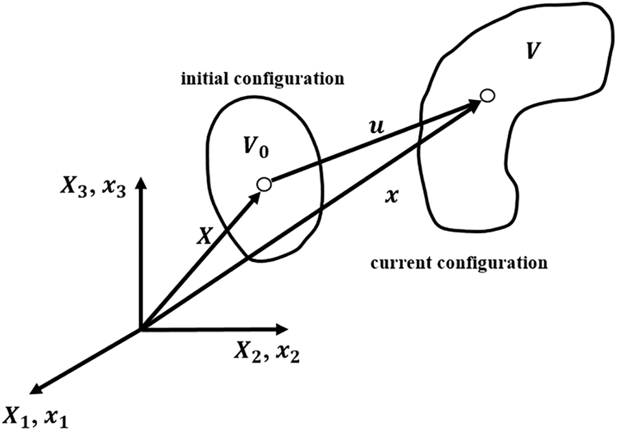
Figure 1: Initial and current configuration

Lagrange description, the equation of motion can be expressed as:

xi=xi(Xj, t),  i, j=1, 2, 3 (2)

The other takes the space coordinate xi and time t as independent coordinates called the space description or Euler description. Solid mechanics mainly adopts the Lagrange material description system. Eq. (2) also shows a single-valued continuous mapping from the initial configuration V0 to the current configuration V. We have:

J=|∂x1∂X1∂x1∂X2∂x1∂X3∂x2∂X1∂x3∂X1∂x2∂X2∂x3∂X2∂x2∂X3∂x3∂X3|=eijk∂xi∂X1∂xj∂X2∂xk∂X3≠0 (3)

Among them,  ∂xi∂Xi is called the deformation gradient, which is an asymmetric second-order tensor, J is called the Jacobin determinant. To examine the changing of the structural micro hexahedron dV0 in the initial configuration, known J=dVdV0=ρ0ρ , ρ0 and ρ represent the density of the medium in the initial and current configurations, respectively, and J=1 when the medium is incompressible.

3.2 Strain Measurement under Large Deformation

Stresses σij and strains εij that are often applied for small deformations are generally referred to as Cauchy stress and Cauchy strain. Since the large deformation motion of an object can be defined concerning different configurations, the description of stress and strain is also different from the case of small deformation [14–16].

3.2.1 Deformation Rate

Consider a typical particle P whose coordinate at time t is xj , and its instantaneous velocity is vi(xj, t) . The coordinate of the particle P′ adjacent to the point P is xj+dxj , and its relative velocity concerning the point P is:

dvi=∂vi∂xjdxj (4)

The equation ∂vi∂xj is called the velocity gradient tensor, which is decomposed into the sum of the symmetric and anti-symmetric parts:

∂vi∂xj=12(∂vi∂xj+∂vj∂xi)+12(∂vi∂xj−∂vj∂xi)=Ωij+Dij (5)

where Ωij is the swirl rate tensor, and Dij is the deformation rate tensor.

It can be shown that the deformation rate tensor Dij is the rate of the Cauchy strain defined concerning the current configuration, the rate εij of the true strain ε˙ij :

Dij=ε˙ij (6)

3.2.2 Green Strain

Green strain tensor [17–19] (Green strain tensor) is defined as:

Eij=12(∂xk∂Xi∂xk∂Xj−δij)=12(∂uj∂Xi+∂ui∂Xj+∂uk∂Xi∂uk∂Xj) (7)

where δij is the Kronecher symbol; ui=xi(Xj, t)−Xj is the displacement vector defined in the initial configuration under small deformation:

∂ui∂Xj ′′1,  ∂∂Xi=∂∂xi (8)

Substitute Eq. (8) into Eq. (7) to get:

Eij=12(∂uj∂xi+∂ui∂xj)=εij (9)

Therefore, in the case of small deformation, the green strain tensor degenerates into a small strain tensor (the Cauchy strain tensor).

3.3 Stress Measurement under Large Deformation

3.3.1 Euler Stress

Divide the force element niΔA acting on the directed surface element ΔTi by ΔA on the current configuration. In the extreme state, we have:

ti(n)=limΔA→0ΔTiΔA=dTidA (10)

The stress vector nidA on the face element ti(n) is represented by the stress vectors on the three face elements perpendicular to the coordinate axes, ti(n)=σijnj (n). σij is the Euler stress tensor, σij is the stress per element area defined on the current configuration, and is the true deformation-related stress.

3.3.2 Piola-Kirchhoff Stress of the First Type (Lagrange Stress)

Definition:

ti∗(N)=limΔA0→0ΔTiΔA0=dTidA0 (11)

In the equation, dA0 is the material surface element on the initial configuration; dTi is the force vector on the current configuration nidA ; ti∗(N) is represented by the coordinates on the current configuration. There are ti∗(N)=∑ij⁡Nj . ∑ij is the Piola-Kirchhoff stress of the first type. It can be inferred from the definition:

∑ij=J∂Xk∂xjσji (12)

3.3.3 Piola-Kirchhoff Stress of the Second Type (Kirchhoff Stress)

Definition:

ti(N)=limΔA0→0ΔTi0ΔA0=dTi0dA0 (13)

In the equation, dTi0=∂i∂xjdTj is the force vector nidA on current configuration dTj the force vector converted to the initial configuration. Therefore, the second type of Piola-Kirchhoff stress [20–22] is defined as:

Skl=∂Xl∂xi ∑ki=J∂Xk∂xi ∂Xl∂xjσij (14)

3.3.4 Jaumann Rate

The strain rate increment is an objective quantity that does not change with the coordinate rotation. The definition:

σij∇=σ˙ij−σipΩjp−σjpΩip (15)

is the Jaumann stress rate [23–25], an objective tensor not affected by the object’s rotation, and is also the stress rate used in ABAQUS.

3.3.5 Truesdell Stress Rate

Taking the material derivative of the Kirchhoff stress concerning time t, we get:

S˙ij=J∂Xi∂xp∂Xj∂xq(σ˙pq+σpq∂vk∂xk−σpk∂vq∂xk−σqk∂vp∂xk) (16)

The expression in the right-hand bracket of Eqs. (2)–(16) is called the Truesdell stress rate, denoted as σ∇T . It can be shown that both the Truesdell stress rate and the Jaumann stress rate are objective tensors that are not affected by rigid body motion.

3.4 Conservation Equation

Thermodynamic systems must satisfy the conservation equations of mass, momentum, and energy [26–28].

3.4.1 Mass Conservation

The mass conservation equation in the Lagrangian description can be expressed as:

ρ(X, t)J(X, t)=ρ0(X) (17)

3.4.2 Momentum Conservation

The definition of momentum shows that the material derivative of the momentum of an object is equal to the sum of the external forces acting on the system, namely:

DDt∫V ⁡ρvi(x, t)dV=∫V ⁡ρbi(x, t)dV+∫A ⁡ti(x, t)dA (18)

Among them, bi is the force acting on the element mass of the object; ti is the surface force. Further derivation of Eq. (18), the differential Equation of motion of the object in the current configuration can be obtained as:

ρDviDt−ρbi−∂σji∂xj=0 (19)

Transform Eq. (19) into the initial configuration to obtain the differential equation of motion of the object in the initial configuration:

ρ0∂vi(X, t)∂t=∂∑ji ∂Xj+ρ0bi (20)

3.4.3 Energy Conservation

If the heat source and heat exchange are not considered, the rate of change of the total energy of the system is equal to the power of the external force, that is:

DDt∫V ⁡(ρwint+12ρvivi)dV=∫V ⁡viρbidV+∫A ⁡vitidA (21)

where wint is the internal energy per element mass. Deriving Eq. (21) can be obtained:

{ ρDwintDt=σijDji=σijε˙jiρ0DwintDt=∑ijFji⋅=∑ijd(∂uj∂Xi)dt​​​​​​​​​​​​​​​​​​​​​​​​​​​​​​​​​ρ0DwintDt=SijE˙ji​​​​​​​​​​​​​​​​​​ (22)

It can be seen from the above equation:

(1)    The Euler stress σij is energy conjugate with respect to the infinitely small strain εij of the current configuration.

(2)    The displacement gradient ∂ui/∂Xj defined by the Lagrange stress ∑ij with respect to the initial configuration is energy conjugated.

(3)    The Kirchhoff stress Sij is energy conjugate with respect to the green strain Eij defined by the initial configuration.

3.5 Numerical Calculation Method of Large Deformation Dynamics

Incremental methods are often investigated when numerical computations involving geometrically nonlinear problems are involved, not only because the problem may involve material inelasticity that depends on the deformation history but also because even if material inelasticity is not involved. However, the incremental method is generally required to obtain the evolution history of stress and deformation during the loading process and ensure the solution’s accuracy and stability. The incremental method discretizes the time variable into a certain time series: t = 0, Δt, 2Δt…, and then obtains the numerical solutions of these discrete time points. Incremental solution methods can be divided into updated Lagrangian and full Lagrangian according to the different reference configurations [29–31]. The updated Lagrangian equation uses the configuration at time t as the reference configuration when calculating all variables in the interval [t, t+Δt] , and the stress-strain measurement adopts Euler stress σij and infinitely small strain εij about the current configuration. The full Lagrangian takes the configuration at t0=0 as the reference configuration. The stress-strain metric uses the Kirchhoff stress Sij and the Green strain Eij defined with respect to the initial configuration.

3.5.1 Update Lagrangian

The controlling equations of the updated Lagrangian are:

Mass Conservation:ρ(X, t)J(X, t)=ρ0(X) (23)

Momentum equation:∂σJI∂xj+ρbi=ρ¨ui (24)

Energy equation:ρwint=σijDji (25)

Deformation rate:Dji=12(∂vj∂xi+∂vi∂xj) (26)

Constitutive relationship:σ∇=σ∇(Dji, σij,  …) (27)

Boundary conditions:{(njσji)|At=t¯tvi|At=v¯i (28)

Initial conditions: u˙(X, 0)=u˙0(X),  u(X, 0)=u0(X) (29)

The momentum Eq. (24) must be satisfied everywhere in the solution domain, and it is almost impossible to solve it directly. The numerical calculation starts from the weak form of the differential equation. It only requires the momentum equation to be satisfied in a certain average sense, and the virtual power equation is derived from this. After the finite element discretization, the node displacement equation is obtained. Taking the imaginary velocity as the weighting coefficient and using the weighted margin method, the weak form of the momentum equation can be expressed as:

∫V δvi(δσijδxj+ρbi−ρu¨i)dV=0 (30)

where δvi (X)∈R0, R0={δvj|δvj∈C0(X),  δvj|Av=0} is the virtual velocity. Using step-by-step integration, Eq. (30) can be written as:

∫V δ(δvi)δxjσjidV−∫V δviρbidV−∫V δvit¯idAt+∫V δviρu¨idV=0 (31)

The above equation is the weak form of the momentum equation, called the virtual power equation. Discretizing the spatial structure, the spatial coordinates of the particle X at any time are:

xi(X, t)=NIxiI(t) (32)

In the equation, NI is the shape function of node I.

The displacement of any particle X in the element can be expressed as the nodal displacement:

ui(X, t)=xi(X, t)−Xi=NI(X)uiI(t) (33)

Similarly, the velocity, acceleration, deformation rate, and virtual velocity of any particle X in the element can be expressed as:

{ u˙i(X,t)=NI(X)u˙iI(t)u¨i(X,t)=NI(X)u¨iI(t)Dij=12(∂u˙j∂xi+∂u˙i∂xj)=12(u˙ji∂NI∂xi+u˙ji∂NI∂xi)=BIuIδvi(X)=NI(X)δviI (34)

Rewrite the above equations into matrix form and substitute them into Eq. (31) to get:

MU¨+fint=fext (35)

Among them, M=∫V ⁡ρNTNdV=∫V0 ⁡ρ0NTNdV0 is the system mass matrix, which is independent of time and only needs to be calculated at the initial moment; fint=∫V ⁡BTσdV;  fext=∫At ⁡NTt¯dA . The nodal displacement uI at the current moment can be obtained by solving Eq. (35), and then the strain and stress of the structure at the current moment can be obtained.

3.5.2 Complete Lagrangian

Different from the updated Lagrangian equation, in the full Lagrangian calculation, the description of the stress and strain adopts the Kirchhoff stress Sij and the green strain Eij defined on the initial configuration. The quantities in the updated Lagrangian format can be converted into the initial configuration using the following:

{σji=δxjδXkδxiδXlSklρbidV=ρ0bidV0t¯idA=t¯i0dA0 (36)

Substitute Eq. (36) into Eq. (35) to obtain the differential equation of motion in the complete Lagrangian format to get the equation:

fint =∫V0⁡B0TSdV0; fext =∫V0⁡NTρ0bdV+∫Ai0⁡NTt¯0dA0; M=∫V0⁡ρ0NTNdV0 (37)

3.6 Basic Solution Method and Solution Process of Large Deformation Dynamic Finite Element

To sum up, the differential equations of motion of the updated Lagrangian method and the complete Lagrangian method can be written as MU¨+fint=fext in the same form. Various direct integration methods, such as the explicit central difference method, implicit Newmark method, etc., can solve the differential equation. The explicit central difference method is the main algorithm used in ABAQUS. For the introduction to the explicit center algorithm, please refer to the related books [32,33], which will not be repeated in this article.

3.7 Single-Point Gaussian Integration and Hourglass Mode

The most serious difficulty of performing nonlinear dynamic analysis is the large-scale and time-consuming calculation. When the explicit integration algorithm is used, the calculation is performed at the element level. There is no need to assemble the total stiffness matrix of the structure and solve the overall balanced equation, so most of the machine time is used to calculate the nodal forces of the element. When single-point Gaussian integration is used, it can greatly save the number of data operations and storage. Still, it may cause hourglass mode [34–37] (or zero-energy mode), leading to calculation divergence and result distortion. Therefore, we must control the hourglass mode. Examining the Equivalent Nodal Vectors in Ordinary Differential Eq. (35):

fint =∫V⁡BTσdV (38)

If the 2×2×2 Gaussian integral is used for the hexahedral element, each element must calculate the constitutive relation eight times. If a single-point Gaussian integral is used, the above equation changes to:

fint =8B0Tσ0J(0, 0, 0) (39)

where B0=B(ξ, η, ζ)|ξ,η,ζ=0, σ0=σ(ξ, η, ζ)|ξ,η,ζ=0, J(0, 0, 0) is the value of the Jacobian determinant of the cell centroid. 8J(0, 0, 0) gives an approximation of the element volume.

The physical interpretation of the hourglass mode is given by taking an 8-node solid element Fig. 2 as an example. The shape function of the 8-node solid element is:

NI(ξ, η, ζ)=18(1+ξIξ)(1+ηIη)(1+ζIζ), I=1, 2, ⋯, 8 (40)

where ξ,  η,  ζ are the natural coordinates of the interpolation point, and ξI,  ηI,  ζI are the natural coordinates of the node I. The velocity of any point in the 8-node solid element is:

vi(ξ, η, ζ)=NI(ξ, η, ζ)viI (41)

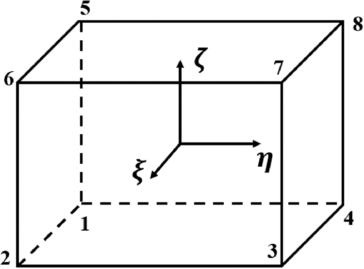
Figure 2: 8-node solid element

In the equation, the repetition index I represents the summation of its values and viI represents the velocity component of the I th node of the element in the xi direction. Substituting Eq. (40) into the above equation, we have:

vi(ξ, η, ζ)=Nvi (42)

Among them:

N=18(ΣT+Λ1Tξ+Λ2Tη+Λ3Tζ+Γ1Tξη+Γ2Tηζ+Γ3Tξζ+Γ4Tξηζ)vi=[ vi1vi2vi3vi4vi5vi6vi7vi8 ]TΣ=[ 11111111 ]TΛ1=[ −111−1−111−1 ]TΛ2=[ −1−111−1−111 ]TΛ3=[ −1−1−1−11111 ]TΓ1=[ 1−11−11−11−1 ]TΓ2=[ 11−1−1−1−111 ]TΓ3=[ 1−1−11−111−1 ]TΓ4=[ −11−111−11−1 ]T

It can be seen from the above equation that the element velocity field is composed of the basis vector Σ, Λ1, Λ2, Λ3, Γ1, Γ2, Γ3, Γ4 . The basis vector Σ reflects the translation of the element, Λ1 describes the tensile and compressive deformation of the element, Λ2, Λ3 describes the shear deformation of the element and Γ1, Γ2, Γ3, Γ4 are called hourglass basis vectors. Fig. 3 shows the hourglass modes of the hourglass in the η direction, and there are 12 hourglass modes in total.

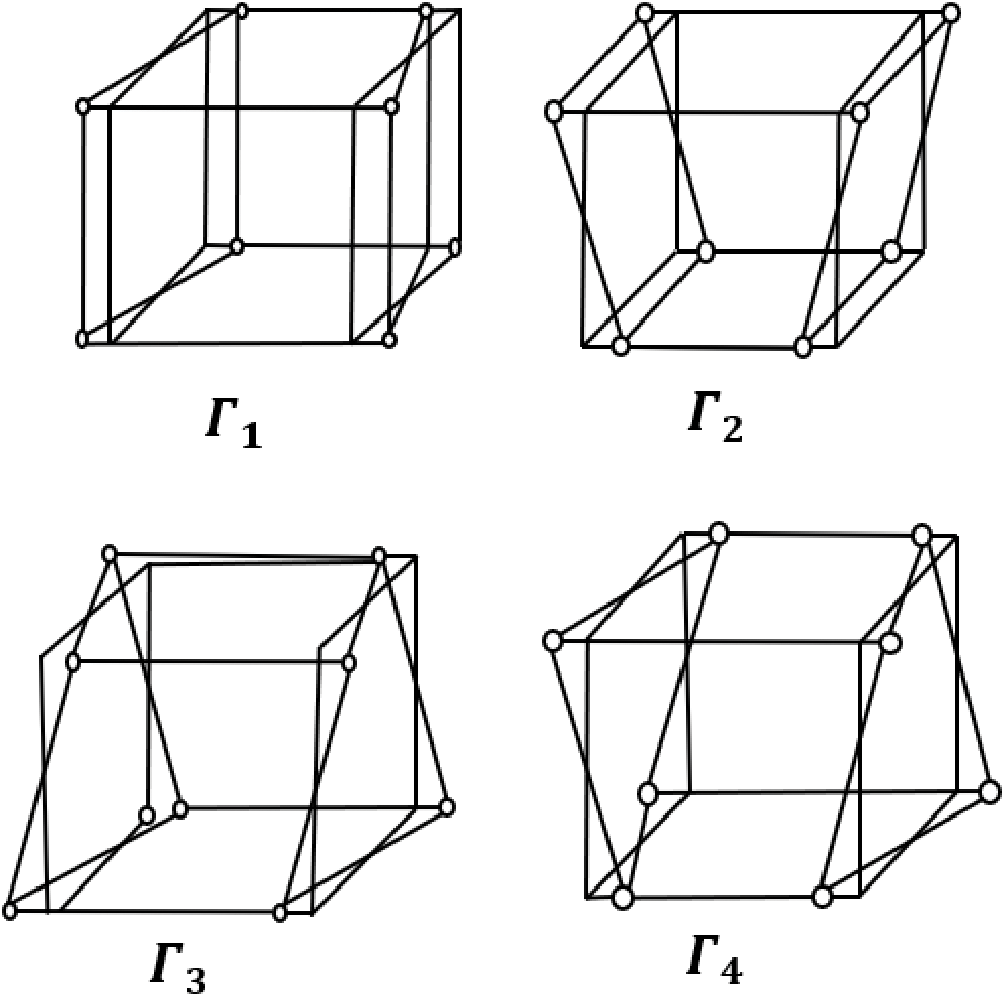
Figure 3: Hourglass mode for an eight-node solid element

The partial derivative of the shape function needs to be calculated when calculating the stress and strain of the element ∂NI/∂x1, ∂NI/∂x2, ∂NI/∂x3 , and need to be obtained by ∂NI/∂ξ, ∂NI/∂η, ∂NI/∂ζ . When a single-point Gaussian integration is performed at the centroid of the cell (ξ, η, ζ=0) , the derivative of the shape function at this location is:

∂N∂ξ=18Λ1T, ∂N∂η=18Λ2T, ∂N∂ζ=18Λ3T (43)

among them, N=[N1N2⋯N8] . The hourglass modes of element deformation are lost during single-point integration Γ1, Γ2, Γ3, Γ4 , i.e., it does not contribute to the element strain energy calculation and is therefore called zero-energy mode. In some cases, the nodal displacement is not zero (that is, the element is deformed), but the strain calculated from the interpolation of the shape function is zero, which is not allowed. If the zero-energy mode is not controlled in the dynamic response calculation, it may develop freely and cause severe numerical oscillations. Two main methods to control the hourglass mode are viscous damping force control and stiffness control [38–41]. In ABAQUS, the former method is mainly adopted. At the element node k, an hourglass viscous damping force is introduced along the xi axis opposite the hourglass modal deformation direction.

fik=−αk∑j=14⁡hijΓjk, i=1, 2, 3, k=1, 2, ⋯, 8 (44)

In the equation, hij=∑k=18⁡vikΓjk is the hourglass mode; the negative sign indicates that the damping force is in the opposite direction to the deformation of the hourglass mode Γjk ; the coefficient is αk=QhgρVe2/3c/4 . In the equation, Ve is the element volume; ρ is the mass density; c is the material sound velocity; Qhg is a user-defined constant, usually taken as 0.05∼0.15. The hourglass viscous damping force of each node is assembled into the overall hourglass viscous damping force matrix H, then the differential equation of system motion can be rewritten as:

Mu˙I+fint =fext+H (45)

Since the hourglass mode is orthogonal to the other basis vectors of the actual deformation, the hourglass mode is continuously controlled during the operation. The work done by the hourglass viscous damping force is negligible in the total energy. This method is simple to calculate and takes less time. The main keywords for hourglass control in ABAQUS are *HOURGLASS” and *HOURGLASS STIFFNESS*. Using explicit integration algorithms facilitates efficient single-point integration, significantly enhancing computational efficiency. This approach negates the necessity of performing multiple integrations per element, substantially curtailing the computational overhead. Notably, the stability condition inherent to explicit schemes provides a robust solution to mitigating issues related to HOURGLASS. Thus, the amalgamation of these characteristics makes explicit integration algorithms an invaluable tool in computational engineering applications.

4  Contact-Collision Nonlinear Problem

4.1 Contact-Collision Algorithm

The collision between two bodies in ABAQUS is achieved by defining contact. ABAQUS generally uses three different algorithms to deal with the contact-collision problem: ABAQUS generally uses three different algorithms to deal with the contact-collision problem Penalty Method, Lagrange Multiplier Method, and Augmented Lagrange Multiplier Method. Penalty Method: The most common method used in ABAQUS for contact-collision problems. It works by adding a penalty force to the equations of motion to prevent penetration of the contact surfaces. Lagrange Multiplier Method: It is also known as the constraint method. It introduces a set of constraints to the equations of motion to prevent penetration of the contact surfaces. Augmented Lagrange Multiplier Method: It combines the penalty and Lagrange multiplier methods. It works by introducing a set of constraints to the equations of motion and adding a penalty force to prevent penetration of the contact surfaces. This method provides more accurate results than the other two methods. The principle is to check whether the slave node penetrates the main surface segment at each time step; a large interface contact force is introduced between the slave node and the penetrated main surface segment, the magnitude of which is proportional to the penetration depth and contact stiffness. Its physical meaning is equivalent to introducing a normal spring between the slave node and the main surface segment to limit penetration, as shown in Fig. 4. The symmetric penalty function rule is to do similar processing for each master node simultaneously.

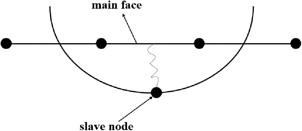
Figure 4: Penalty function algorithm schematic

4.2 Numerical Calculation Method of Contact-Collision

4.2.1 Contact and Non-Embedded Conditions

Considering the contact problem of objects A and B, their current configurations are denoted as VA and VB, respectively. The boundary surfaces are denoted as AA and AB, and the contact surface is denoted as AC = AA ∩ AB, as shown in Fig. 5.

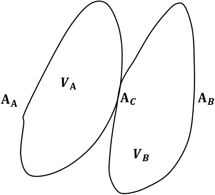
Figure 5: Contact between two objects

Object A is the master, its contact surface is the master surface, object B is the enslaved, and its contact surface is the slave surface. The non-embedding conditions [42] for objects A and B can be expressed as:

VA∩⁡VB=0 (46)

The above equation shows that objects A and B cannot overlap. Since it is impossible to determine where the two objects are in contact in advance, the non-embedded condition cannot be expressed as an algebraic or differential displacement equation in the large deformation problem. It can only be compared at each step. The coordinates of the corresponding nodes of objects A and B on the surface Eq. (47) or the contrast rate Eq. (48) to achieve the displacement coordination condition:

UNA−UNB=(uA−uB)nA≤0|AC (47)

VNA−VNB=(vA−vB)nA≤0|AC (48)

In the equation, the subscript N represents the contact’s normal direction.

4.2.2 Contact Force Conditions

By Newton’s third law, the contact force should satisfy the following:

{tNA+tNB=0tTA+tTB=0 (49)

where tNA, tNB represent the normal contact force of object A and object B, respectively. tTA, tTB are the tangential contact force (i.e., frictional force) of objects A and B, respectively.

4.3 Finite Element Implementation of Contact Collision Algorithm

The calculation steps of the symmetric penalty function [43,44] are as follows:

(1)   As shown in Fig. 6, search for the closest master node mS to any slave node nS .

(2)   Check the main surface segments associated with the master node mS , and determine the main surface segments that the slave node nS may contact when penetrating the main surface. If the master node mS does not coincide with the slave node nS , when the following two inequalities are satisfied, the slave node nS maybe in contact with the master surface segment Si :

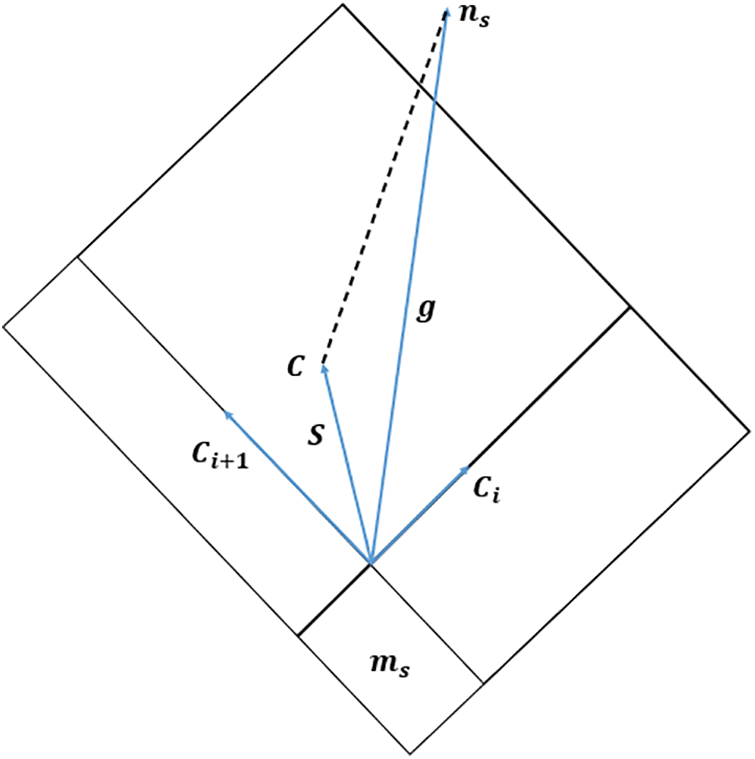
Figure 6: Contact between slave node and master surface segment

{(Ci×S)⋅(Ci×Ci+1)>0(Ci×S)⋅(S×Ci+1)>0 (50)

In the equation, the Ci and Ci+1 vectors are the two edge vectors at the point mS on the main face segment Si ; the vector S is the projection of the vector g on the main surface; g is the vector from the master node to the slave node nS .

S=g−(g⋅m)m (51)

In the equation:

m=CiCi+1/|CiCi+1| (52)

where the vector m is the outer normal element vector of the principal face segment. If the slave node is close to or located on the intersection of two main surface segments, the above inequality may be uncertain, and S takes the maximum value at this time.

S=max(gCi/|Ci|)i=1, 2, ⋯ (53)

(3)   Determine the position of the possible contact point c of the slave node nS on the main surface segment Si . The position vector r of any point on the main surface segment Si can be expressed as:

r=f1(ξ, η)i1+f2(ξ, η)i2+f3(ξ, η)i3 (54)

where fi(ξ, η)=∑j=14⁡ϕj(ξ, η)xij, ϕj(ξ, η)=14(1+ξjξ)(1+ηjη) , xij is the coordinate value of the node j for the element; i1, i2, i3 is x1, x2, x3 , the element vector of the axis. The contact points c(ξc, ηc) the location must satisfy the following two equations:

{δrδξ(ξc, ηc)⋅[t−r(ξc, ηc)]=0δrδη(ξc, ηc)⋅[t−r(ξc, ηc)]=0 (55)

(4)   Check whether the slave node penetrates the master surface segment.

If the following equation holds:

l=ni[t−r(ξc, ηc)]<0 (56)

Then it means that the slave node nS penetrates the main surface segment Si containing the contact point c(ξc, ηc) . Where ni is the outer normal line element vector of the main surface segment at the contact point c, and its calculation equation is:

ni=δrδξ(ξc, ηc)×δrδη(ξc, ηc)|δrδξ(ξc, ηc)×δrδη(ξc, ηc)| (57)

If l ≥ 0 , the slave node nS does not penetrate the main surface segment, the two objects do not touch-collide, so no processing is performed, and the search for the slave node nS ends, and the search for the next slave node nS+1 begins. The relationship between the slave node and the master segment is shown in Fig. 7.

(5)   If the slave node penetrates the main surface segment, a normal contact force is applied between the slave node nS and the contact point c.

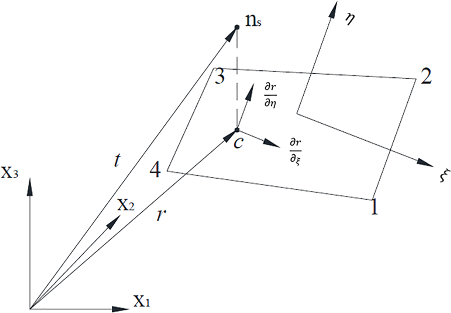
Figure 7: The relationship between the slave node and the master segment

fS=−lkini (58)

In the equation, ki is the stiffness factor of the main face segment Si , and its calculation equation is:

ki=fKiAi2/Vi (59)

where Ki , Vi and Ai are the bulk modulus, volume, and area of the main surface segment of the element where the main surface segment Si is located; f is the contact stiffness scaling factor, and the default value is 0.1. During the calculation of ABAQUS, if the penetration is too large, the user can increase the penalty function factor in the contact definition within ABAQUS. This can be done by increasing the “Penalty” parameter within the “Contact Interaction” or “Contact Pair” definition. Increasing the penalty factor will increase the stiffness of the contact, making it less likely for penetration to occur. However, increasing the penalty too much can lead to unrealistic results and numerical instability, so it should be done with caution and testing. If the value of f is too large (>0.4) , the numerical calculation may be unstable unless the time step is reduced. The normal contact force vector fS is applied to the slave node nS , and then, according to Newton’s third law, a force in the opposite direction fS is applied to the contact point  c of the main surface segment. The contact force at point c can be equally distributed to the nodes of the main surface segment according to the following equation:

fjm=−ϕj(ξc, ηc)fS, j=1, 2, 3, 4 (60)

ϕj(ξc, ηc) is a two-dimensional shape function on the main surface segment, and there is ∑j=14⁡ϕj(ξc, ηc)=1 at the contact point “c”.

(6)   Calculation of tangential contact force (friction force) If the normal contact force from node nS is fS , then the maximum friction force is FY=μ|fS|, and μ is the friction coefficient. Assuming that the friction force of the slave node nS at the last moment tn is Fn , then the friction force (probing friction force) that may be generated at the current moment tn+1  (trial friction force) F∗ for F∗=Fn−kΔα, Δα=rn+1(ξcn+1, ηcn+1)−rn+1(ξcn, ηcn), k is the interface stiffness. The following equation calculates the frictional force at the current moment:

Fn+1={F∗|⇒ |F∗|≤FYFYF∗/|F∗|⇒ |F∗|>FY (61)

Finally, the friction force of the four main nodes corresponding to the main surface segment is calculated according to the theorem of action force and reaction force. If the coefficient of static friction is μs and the coefficient of dynamic friction is μd , the exponential interpolation function is used to make a smooth transition between the two:

μ=μd+(μs−μd)e−C|V| (62)

where V=Δe/Δt, Δt is the time step, and C is the decay factor. In ABAQUS, friction can be activated in a contact interaction by defining the friction coefficient as a non-zero static ( FS ) and dynamic ( Fd ) friction coefficients in the input file’s *CONTACT* definition section or the ABAQUS/CAE interface by specifying the friction coefficient in the contact properties. The contact properties can also define the type of friction (e.g., Coulomb or viscous). If the static and dynamic friction coefficients are not equal, FS should be greater than Fd , and a non-zero attenuation coefficient Dc must be specified. For problems with numerical noise, such as collision, FS and Fd are generally set to the same value to avoid additional noise.

(7)   Take the contact force vectors fS , fjm , and friction force vectors as known vectors, and assemble them into the overall load vector-matrix P for dynamic analysis.

The symmetric penalty function algorithm lends the above algorithm to the slave node and master node, respectively.

4.4 Material Nonlinear Problems

Material nonlinear problems can be divided into two categories [45–47]. The time-independent elastoplastic problem is characterized by material deformation occurring immediately after the load is applied and does not change with time. The other type is the time-dependent viscous problem, characterized by the fact that the material undergoes corresponding elastic-plastic deformation immediately when the load is applied.

The deformation continues to change with time. The ABAQUS program primarily considers materials’ nonlinear and rate-dependent effects through built-in material models. The contact algorithm, mesh density, boundary conditions, and loading approximations were validated through sensitivity studies, which verified the variability induced by these assumptions was within an acceptable tolerance of less than 10% for key output measures.

5  Applicability of the Nonlinearity Experimentally

In this section, numerical simulations investigate the dynamic response and failure modes of reinforced concrete (RC) members under asymmetrical impact loads. A collision between a rigid hammer and an RC member is simulated using the explicit central difference algorithm of ABAQUS, a commercial finite element software. Parameters include the mass of the hammer, its initial velocity, and the axial compressive strength of the concrete feature in this simulation. Furthermore, an analysis is carried out to examine various parameters’ effects on the RC members’ dynamic response and their failure modes under asymmetrical impact load. Specific elements under investigation include the influence of the longitudinal and stirrup reinforcement ratios. These simulations provide insights into how different factors, including the characteristics of the impact load and the properties of the RC member, impact the member’s dynamic response and failure modes. The results from this investigation bear significant implications for the design and safety assessment of RC structures subject to impact loads.

5.1 Model Definition

Utilizing ABAQUS, a 3D split model of a group of square reinforced concrete (RC) members is created (as depicted in Fig. 8).

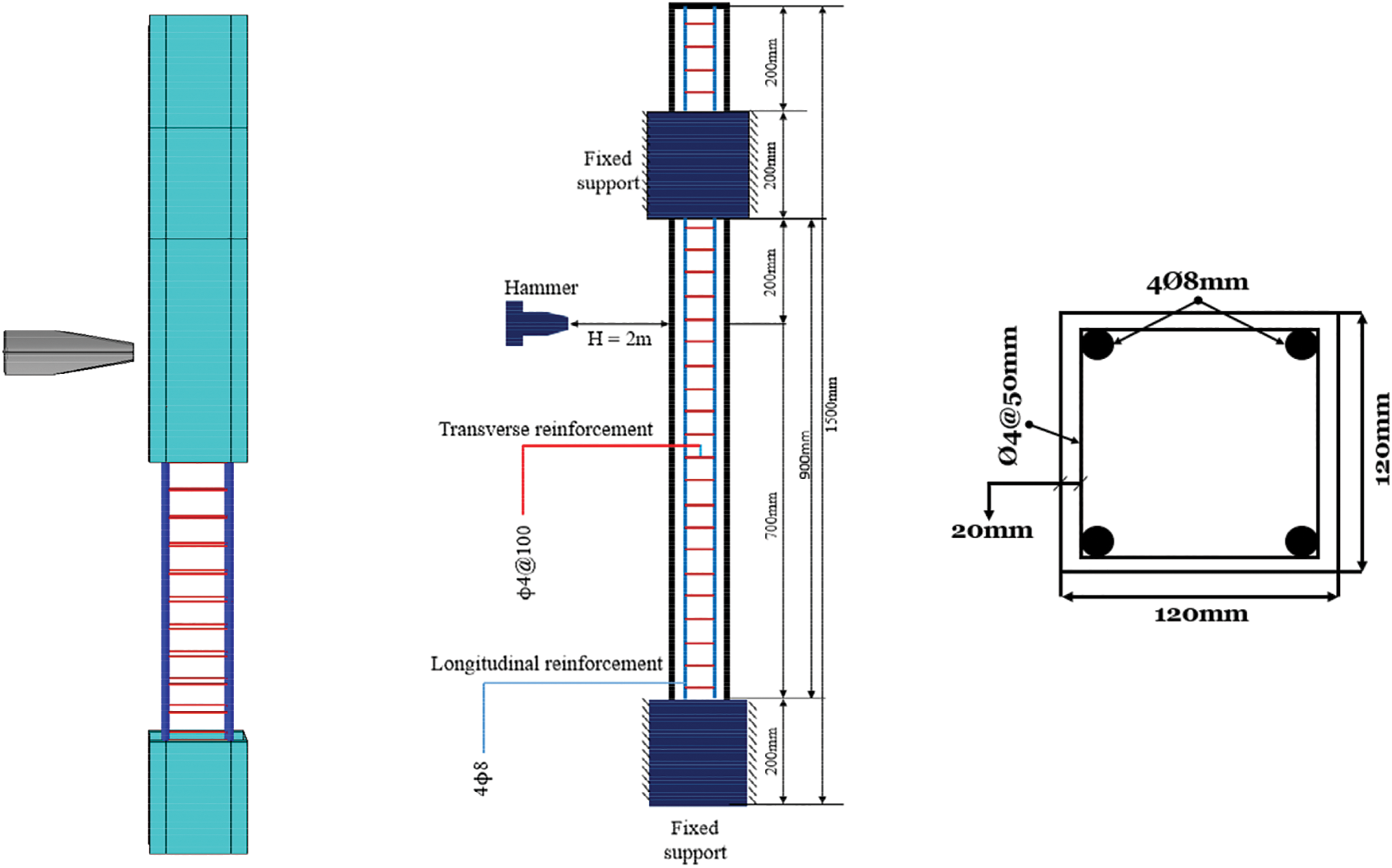
Figure 8: Finite element model of RC member

The bond-slip is considered in the connection between the reinforcement and the concrete. Key dimensions of the RC member include section height (h = 120 mm), section width (b = 120 mm), member net height (H = 1.5 m), and the thickness of the concrete cover (c = 20 mm), as shown in Fig. 8. The boundary conditions of the finite element model can be simplified to fix both the top and bottom surfaces of the member. This means the top and bottom surfaces cannot move horizontally or vertically. In other words, the top and bottom surfaces are rigidly fixed. While this assumption may slightly restrict displacements near the supports, prior studies have validated that the key impact behaviors remain accurately captured with fixed ends.

5.2 Material Model

The model can be shortened to the sphere is rigid (*ELASTIC), reinforcements use *PLASTIC_KINEMATIC and strain rate effects are included [32,48]. While more complex plasticity models could offer enhanced strain rates and work hardening behaviors, the chosen approach captures essential nonlinearity while reducing computational expenses. The steel yield stress can be expressed as:

σy=[1+(ε˙C)1p](σ0+βEpεeffp) (63)

where σ0 is the initial yield stress of the reinforcement; p, C are the strain rate parameters of the Cowper-Symonds model; β is the parameter for adjusting isotropic strengthening and kinematic strengthening; Ep is the plastic hardening modulus; εeffp is the effective plastic strain. The material parameters used for the reinforcement in this paper are shown in Table 1.

The concrete material can be summarized as concrete uses (Concrete Damaged Plasticity), strain rate effects are included using the DIF (dynamic/static strength ratio), CDIF coefficient from the improved K&C model, and Eqs. (64) and (65):

CDIF=fcdfcs=(ε˙dε˙cs)1.206α(ε˙d≤30s−1) (64)

CDIF=fcdfcs=γ(ε˙d)1/3(ε˙d>30s−1) (65)

where fcd is the concrete dynamic compressive strength, ε˙d the strain rate, fcs is the concrete static compressive strength (compressive strength of concrete at ε˙cs=30×10−6S−1 ); log⁡γ=6.156α−0.49 , where α=(5+3fcu/4)−1 , fcu is the concrete cube’s compressive strength. The increase factor TDIF of concrete tensile strength is determined by Eqs. (66) and (67).

TDIF=ftdfts=(ε˙dε˙ts)δ(ε˙d≤1s−1) (66)

TDIF=ftdfts=β(ε˙dε˙ts)1/3(ε˙d>1s−1) (67)

where ftd is the concrete dynamic tensile strength at the strain rate ε˙d , where fts concrete static tensile strength ( ε˙ts=10−6S−1 concrete tensile strength); log⁡β=6δ−2 , where: δ=(1+8fc′/fc0′)−1 , fc0′=10 MPa , fc′ axial compressive strength of concrete under quasi-static conditions.

The concrete parameters are curves generated from the K&C model, and the other parameters are ABAQUS default [48].

5.3 Contact of Reinforcement to Concrete

The bond-slip model defines the concrete using a 3D stress element (C3D8R). The reinforcement is modeled using truss elements (T3D2). The interaction between the concrete and the reinforcement is governed by a (*CONTACT PAIR) definition with (slip) behavior, with the reinforcement nodes serving as the slave side and the concrete nodes as the master side. The bond between the reinforcement and the concrete is modeled as being proportional to the slip until a maximum limit, beyond which separation occurs. This frictional behavior is defined using a (*FRICTION) definition, which provides the frictional stress vs. slip rate behavior. Bond-slip relationship elastic stage is linear, the plastic stage is exponential decay, and damage accumulation is considered an elastic stage linear relationship and the plastic stage as exponential decrease.

τ={GsSS≤Smaxτmaxe−hdmg Ds>Smax (68)

where Gs is the bond shear modulus; hdmg  is the damage index curve coefficient; Smax is the maximum elastic slip; D is the damage parameter, representing the accumulation of plastic strain according to Yao et al.’s literature [49]. The parameter values used in this paper are: Gs=50MPa/mm , hdmg =0.2, Smax=0.36 mm.

5.4 Bond-Slip Model Verification

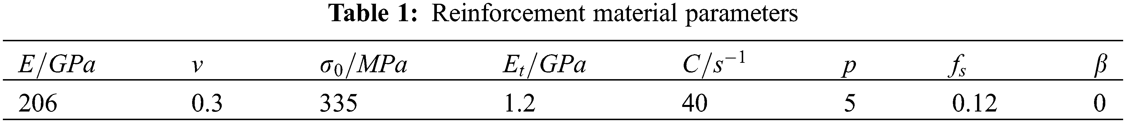
Two models were established to validate the bond-slip model: (1) The proposed bond-slip model. (2) A standard model using common nodes. However, the model parameters are as follows:

Hammer mass: 270 kg, initial velocity: 2 m/s, concrete strength fc′=45.4MPa , reinforcement: 4∅8 longitudinal, ∅ 4@100 mm stirrups. Fig. 9 compares the horizontal displacement at the asymmetric point. The peak displacements from the two models show good agreement, bond-slip model 120.9 mm and common node model 115.3 mm within a 5% difference. The displacement-time curves from the two models exhibit similar trends. However, the residual displacements differ slightly due to how the models capture slips. The energy response of the simulation provides an important validity check. Fig. 10 shows that nearly all (97%) of the initial kinetic energy is converted to internal, hourglass, and other energies.

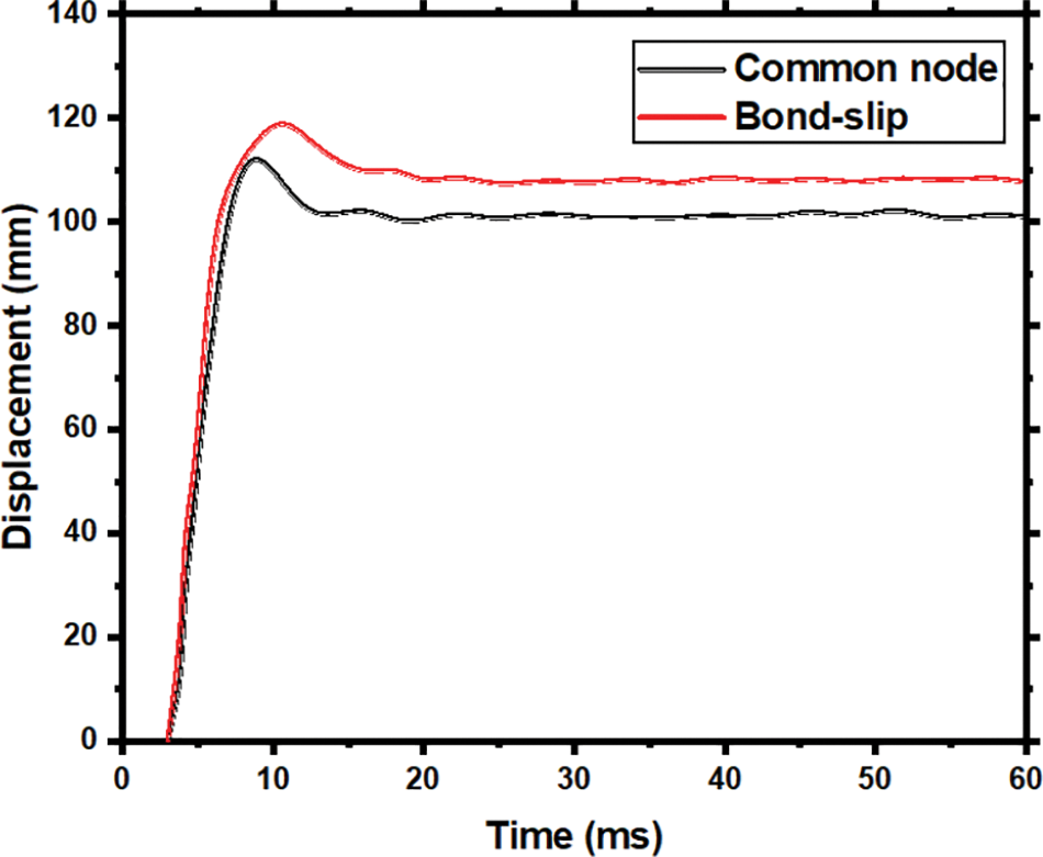
Figure 9: Comparison of horizontal displacement of members under two methods

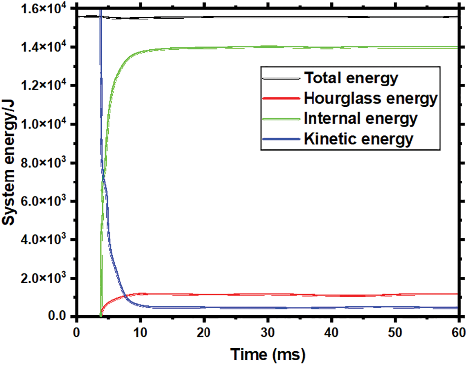
Figure 10: System energy curve for the member under asymmetrical impact force

The total energy is conserved, indicating an accurate solution. The hourglass energy remains below 10% of the internal and total energies. This demonstrates that hourglass control is effective, and the results are reliable, as reported in previous studies. In summary, the reasonable energy conversion and controlled hourglass energy provide confidence that the proposed bond-slip method captures the member response accurately. The energy check thus corroborates the model validation based on displacement comparisons, demonstrating the validity and reasonableness of the bond-slip method.

5.5 Dynamic Response Analysis

The dynamic response of RC members is further studied by analyzing the effects of various parameter values using the bond-slip model mentioned above.

5.5.1 Rigid Sphere Mass

Fig. 11 demonstrates the influence of varying hammer mass on the horizontal displacement at the asymmetrical point of the RC member, maintaining all other parameters as in Section 5.4. An increase in hammer mass results in a gradual increase in peak and residual displacements. However, the rate of these increases experiences a diminishing trend. For instance, a mass increase from 220 to 270 kg causes a 33 mm peak displacement increase, which reduces to 27 mm when mass increases from 270 to 310 kg. This suggests that while larger hammer masses elicit greater structural responses, the development speed of the RC member’s plastic region decelerates with mass increase.

Figure 11: Comparison of the horizontal displacement of RC members under different sphere hammer masses

5.5.2 The Initial Velocity of the Sphere Hammer

Fig. 12, with parameters as in Section 5.4, reveals that increasing the hammer mass incrementally elevates the peak and residual displacements of the RC member’s asymmetrical point, albeit at a declining rate. For example, a peak displacement increase of 33 mm occurs when mass rises from 220 to 270 kg, which lessens to 27 mm from 270 to 310 kg.

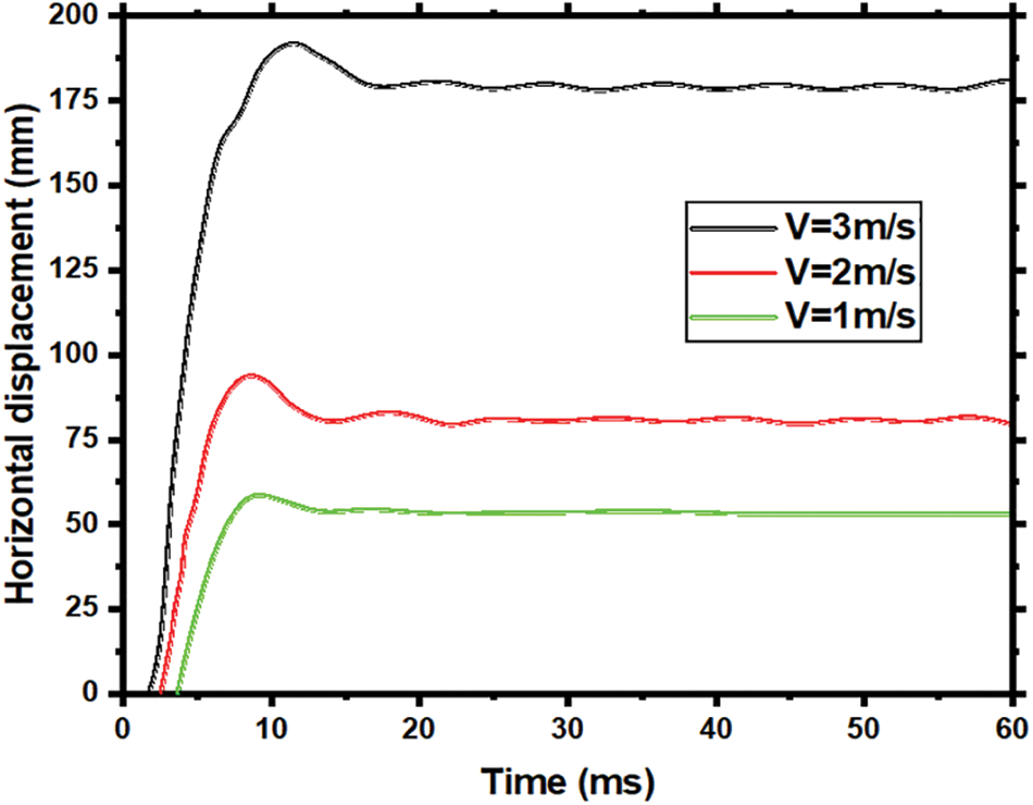
Figure 12: Comparison of the horizontal displacement of RC members under different sphere hammer velocities

This implies that larger hammer masses amplify structural responses but also decelerate the development of the RC member’s plastic region. Fig. 12 presents the horizontal displacement of an RC member’s asymmetrical point under varying initial velocities of a rigid hammer impact. The same model parameters from Section 5.4 are applied. As the initial hammer velocity increases, the peak value and residual displacement exhibit a nonlinear acceleration. Specifically, a jump from 1.0 to 2.0 m/s increases peak displacement by 35.4 mm, while a leap from 2.0 to 3.0 m/s results in a 97.6 mm increase. This indicates a continuous increase in the RC member’s displacement response and a quicker development of the member’s plastic zone as the initial hammer velocity increases.

5.5.3 Axial Compressive Force

The impact of axial compressive strength on the dynamic response of RC members was studied using rigid hammer simulations on three members with strengths of 30, 40, and 50 MPa. The hammer mass (m = 270 kg), initial velocity ( v=2m/s ), and other parameters were maintained per Section 5.4. Fig. 13a depicts the horizontal displacement at the asymmetrical point for members with different axial compressive strengths using the same strain rate effect curve (at fc′=50MPa ). Increasing axial strength reduces the peak and residual displacements to varying extents. Higher strength under identical load levels decreases the area of concrete member entering plasticity, reducing horizontal displacement at the member’s asymmetrical point. Fig. 13b presents a time-history curve comparison of horizontal displacement at the RC member’s asymmetrical point under various axial compressive strengths, considering strain rate effects. The strength increases the coefficient DIF, a function of fc′ (the calculation method in Section 5.2), does not effectively diminish peak or residual displacement magnitude amidst increased concrete axial strength. Lower-strength materials show heightened strain rate sensitivity and a higher DIF at the same strain rate [50]. Therefore, dynamic responses of low-strength concrete structures may be lower than high-strength ones (verifiable by comparing Figs. 13a and 13b). Thus, concrete strength selection for anti-collision structures should be reasonable, within specification limits, without defaulting to high-strength concrete.

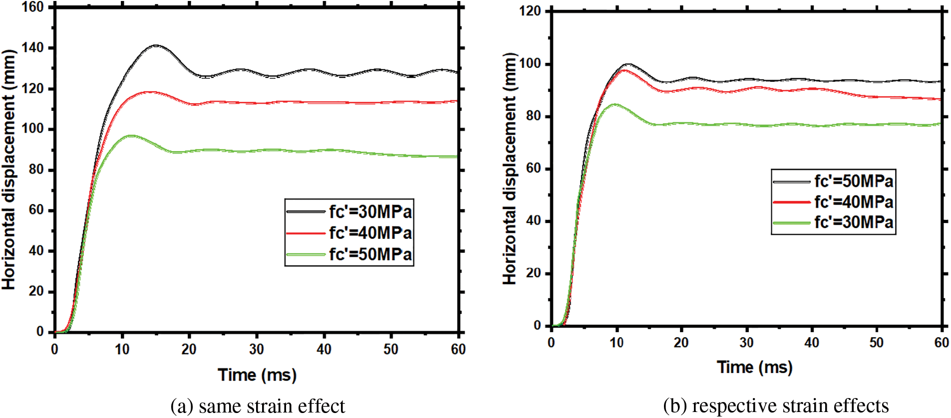
Figure 13: Comparison of the horizontal displacement of RC members under different concrete axial compressive strengths with different strain effects

5.5.4 Longitudinal Reinforcement Ratio

Maintaining all parameters as in Section 5.4 and varying only the longitudinal reinforcement ratio, Fig. 14 indicates a reduction in peak and residual displacements at the asymmetrical point with an increasing reinforcement ratio. This reduction becomes particularly pronounced when the ratio increases from 0.016 to 0.019. Enhanced flexural and shear resistance due to higher reinforcement ratios results in a smaller area entering the plastic state under a consistent load level, effectively reducing the RC member’s displacement at its asymmetrical point.

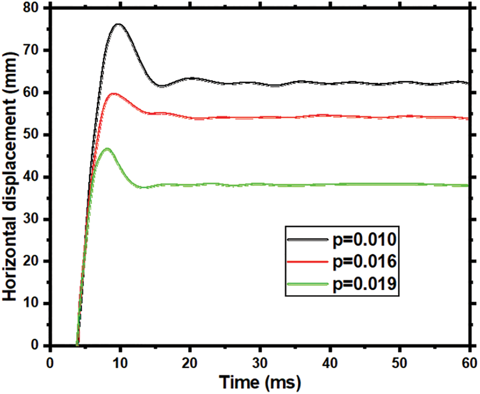
Figure 14: Comparison of the horizontal displacement of RC members under different longitudinal reinforcement ratios

5.5.5 Ratio of Stirrups

Fig. 15 compares time-history curves of horizontal displacement at the asymmetrical point under two stirrup reinforcement ratios, 0.002 (s = 200 mm) and 0.005 (s = 80 mm), with other parameters as in Section 5.4. Fig. 15 shows an 18% and 30% reduction in peak and residual displacements, respectively, when the ratio increases from 0.002 to 0.005. This suggests that augmenting the stirrup reinforcement ratio enhances shear resistance and reduces displacement at the member’s asymmetrical point. Additionally, decreased stirrup spacing better restrain core concrete deformation.

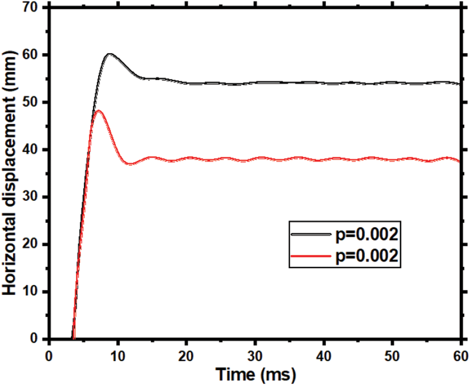
Figure 15: Comparison of the horizontal displacement of RC members under different stirrup reinforcement ratios

5.5.6 Failure Mode Analysis

Under asymmetrical impact load, RC members exhibit two primary failure modes: local and overall. Local failure involves crushing concrete in the impact area (Fig. 16a) and cracking and spalling away from the impact side (Fig. 16b) caused by the instantaneous impact force. The surface pressure of the colliding body generates high internal stress in the contact area, resulting in concrete crushing. Concurrently, large deflection and deformation induce excessive tensile stress on the far side of the impact, destroying the bond between reinforcement and concrete and leading to concrete cracking and spalling.

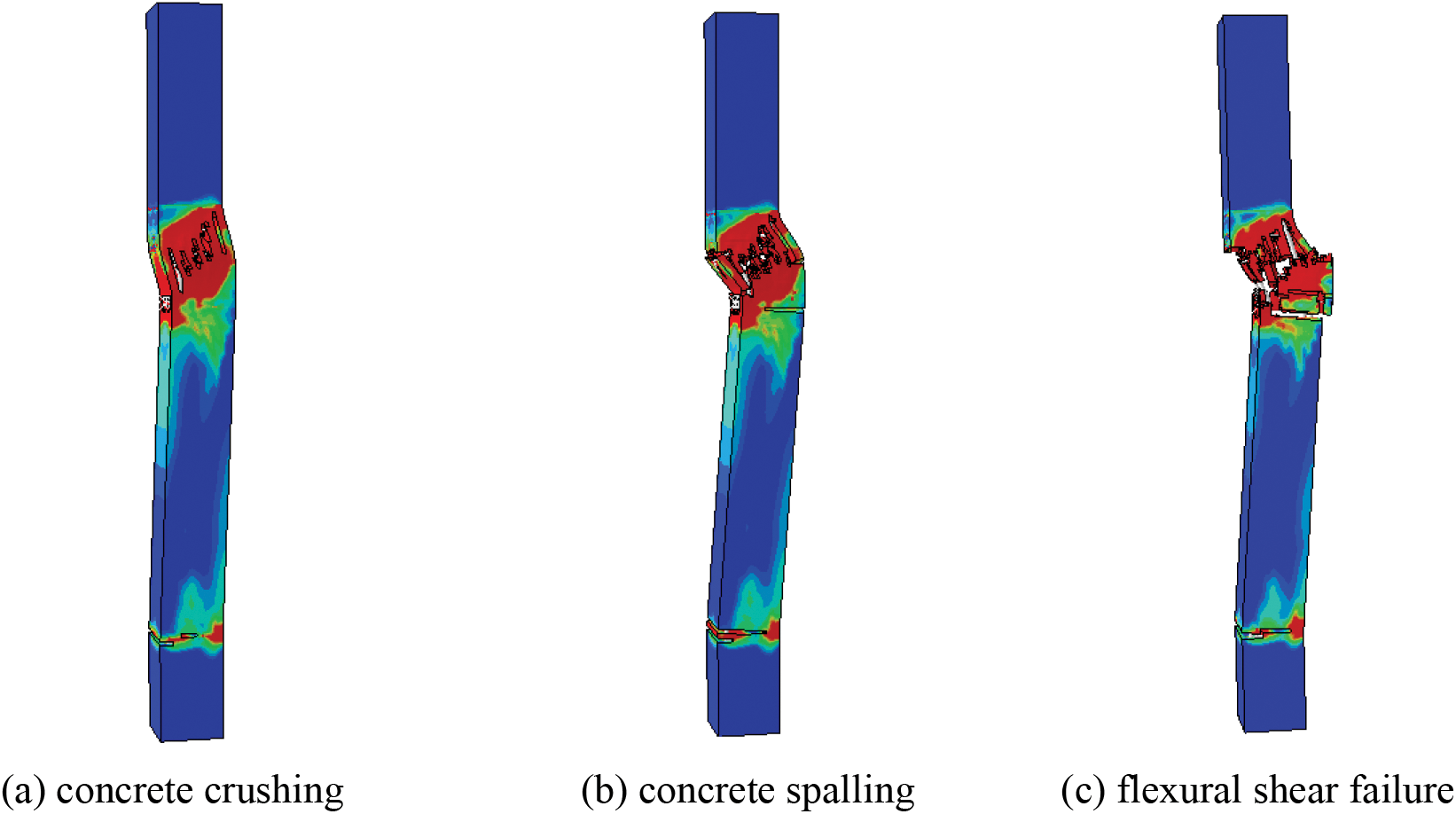
Figure 16: The failure mode of RC members under asymmetrical impact load

Numerical simulations revealed that under asymmetrical impact load, overall RC member failure primarily manifests as bending shear failure (Fig. 16c), with bending deformation fully developed before the onset of shear deformation. This overall failure is closely tied to the type of impact load. Impulse loads with high peaks and short durations often result in shear failure as the member’s shear stress rapidly reaches failure stress before effective bending deformation occurs. Conversely, quasi-static loads with low peaks and longer durations tend to induce bending failure due to effective bending deformation development. Collision impact loads between impulse and quasi-static loads typically lead to bending shear failure, falling under dynamic load classification.

6  ABAQUS Program Reliability and Accuracy Verification

ABAQUS is a popular and widely used finite element analysis (FEA) software program known for its reliability and accuracy. Verifying the reliability and accuracy of ABAQUS is an important step in ensuring that simulations performed using the program are accurate and trustworthy. One way to verify the reliability of ABAQUS is to compare the results of simulations performed using the program to experimental data or analytical solutions. This can be done by comparing the results of a simulation to the results of a physical test or by comparing the results of a simulation to an analytical solution for a known problem. The program can be reliable if the simulation results agree with the experimental data or analytical solution. In addition to performance tests, sensitivity studies can verify ABAQUS’ accuracy. A sensitivity study involves varying one or more input parameters and comparing the results to the original simulation. This can help identify any areas where the simulation is sensitive to changes in input parameters and can also help identify any areas where the simulation is inaccurate. It is also important to verify the robustness of the software by performing benchmark tests and comparing the results to other codes and standards. This can be done by running simulations of known problems and comparing the results to other simulations performed using other software programs or analytical solutions. In addition to the above, the proper meshing technique used in the simulation also plays a crucial role in ensuring the reliability and accuracy of ABAQUS. A good mesh reduces the number of elements required for the simulation, increases the degree of freedom, and reduces the computation time. The ABAQUS program is a full-featured geometric nonlinear, contact nonlinear, and material nonlinear analysis software. It is mainly based on the Lagrange algorithm and has both ALE and Euler algorithms; it is mainly based on an explicit solver and has both implicit solver functions. It is mainly based on structural analysis and has thermal analysis and fluid-structure coupling functions; it is mainly based on nonlinear dynamic analysis and has static analysis functions; it is a general nonlinear finite element program for structural analysis [48,51].

6.1 Problem Statement

The impact of elastic rods is a classic case in the contact problem, studied by many scholars and obtained theoretical, analytical solutions [52–56]. For more discussion about the contact problem, one example of the elastic rod under impact load will be used for simulation by ABAQUS and compare the output with the theoretical and analytical solutions. The reinforced concrete RC column is a composite concrete and steel reinforcement material. The steel reinforcement gives the column additional strength and ductility, making it more resistant to bending, compression, and other loads. It is worth noting that this example is harder and more complex than using other materials like a rod because it involves the behavior of a composite material, it is more difficult to solve analytically, and it is more common to use numerical methods such as FEA to simulate the collision. The impact of elastic rods is a classic case in contact mechanics, which deals with the behavior of bodies in contact with one another. The problem involves the collision of two elastic rods, and the goal is to determine the forces and deformations that occur during the impact. Many scholars have studied this problem and developed several theoretical and analytical solutions [57–61]. One such solution is provided by the finite element software ABAQUS, widely used in engineering and scientific research to simulate the behavior of structures under various loading conditions.

6.2 ABAQUS Modeling

ABAQUS can be used to model the impact of elastic rods by creating a simulation of the collision and solving the resulting system of equations using numerical methods. Problem description: the impact of two homogeneous elastic rods, Rod A and Rod B, is being studied. Rod A moves with an initial velocity of 1 m/s and collides with a static Rod B. Both rods are made of the same material, with an elastic modulus of 100 Pa, Poisson’s ratio of 0.3, a density of 0.01 kg/m3, a cross-sectional area of 1 m2, and a length of 10 m. The ends of Rod A and Rod B were constrained to prevent translational and rotational displacement. Specifically, the ends were fixed against motion in the x, y, and z directions and rotation about the x, y, and z axes. This simplified boundary condition restricts the rods from moving horizontally or vertically at their ends while still allowing wave propagation, which has been shown in prior studies to accurately capture the stress wave behavior during rod impacts. The goal of the problem is to determine the forces and deformations that occur during the impact of these two rods and use this information to understand the behavior of the rods during the collision. This problem can be solved using analytical or numerical methods, such as finite element analysis with software such as ABAQUS. It can provide valuable insights into the mechanics of rod impacts, which can be useful in various engineering applications.

6.3 Simulation and Results

A highly refined finite element mesh is utilized to analyze the propagation of stress waves resulting from the impact of Rods A and B. This mesh is densely divided, as illustrated in Fig. 17, to ensure an accurate investigation of the stress wave behavior.

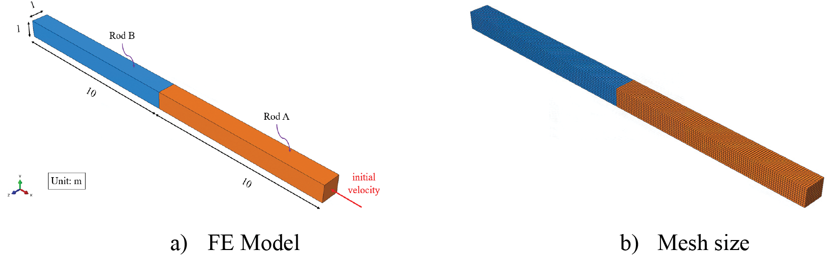
Figure 17: Finite element model simulation

The stress wave propagation in Rods A and B during the impact process was investigated. Figs. 18a–18c show the axial stress contours of the rods at 0.01, 0.02, and 0.04 s, respectively, where zero sec is the initial velocity assumed in the analytical solution is 0 for both rods for simplicity.

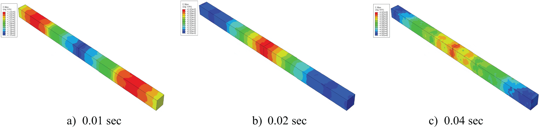
Figure 18: Stress wave propagation contour

Fig. 17a shows the initial contact between Rod A and Rod B. At this early stage of impact, the stress has not had sufficient time to propagate along Rod B, so its distal end furthest from the impact point remains unaffected and experiences a limited stress range close to zero. As the impact time increases, the stress wave, also known as the loading or compression wave, propagates from the contact impact face to the distal free surface of the rod, beginning to reach the surface, as shown in Fig. 18b. While the stress wave beginning to reach the free surface is seen at 0.02 s in Fig. 18b, the total propagation time may be longer than depicted in Fig. 19. The compression of both rods occurs at this point, and the stress wave is reflected on the free surface at the far end, changing from a compression wave to a tensile wave. This results in tensile stress waves at the distal ends of Rods A and B, as shown in Fig. 18c. The stress propagation shown here at 0.01, 0.02, and 0.04 s corresponds to the times analyzed in Fig. 19. These stress wave propagation laws align with the theory of one-dimensional elastic waves [62]. Notably, using ABAQUS software to analyze contact collision problems is reliable and proven effective.

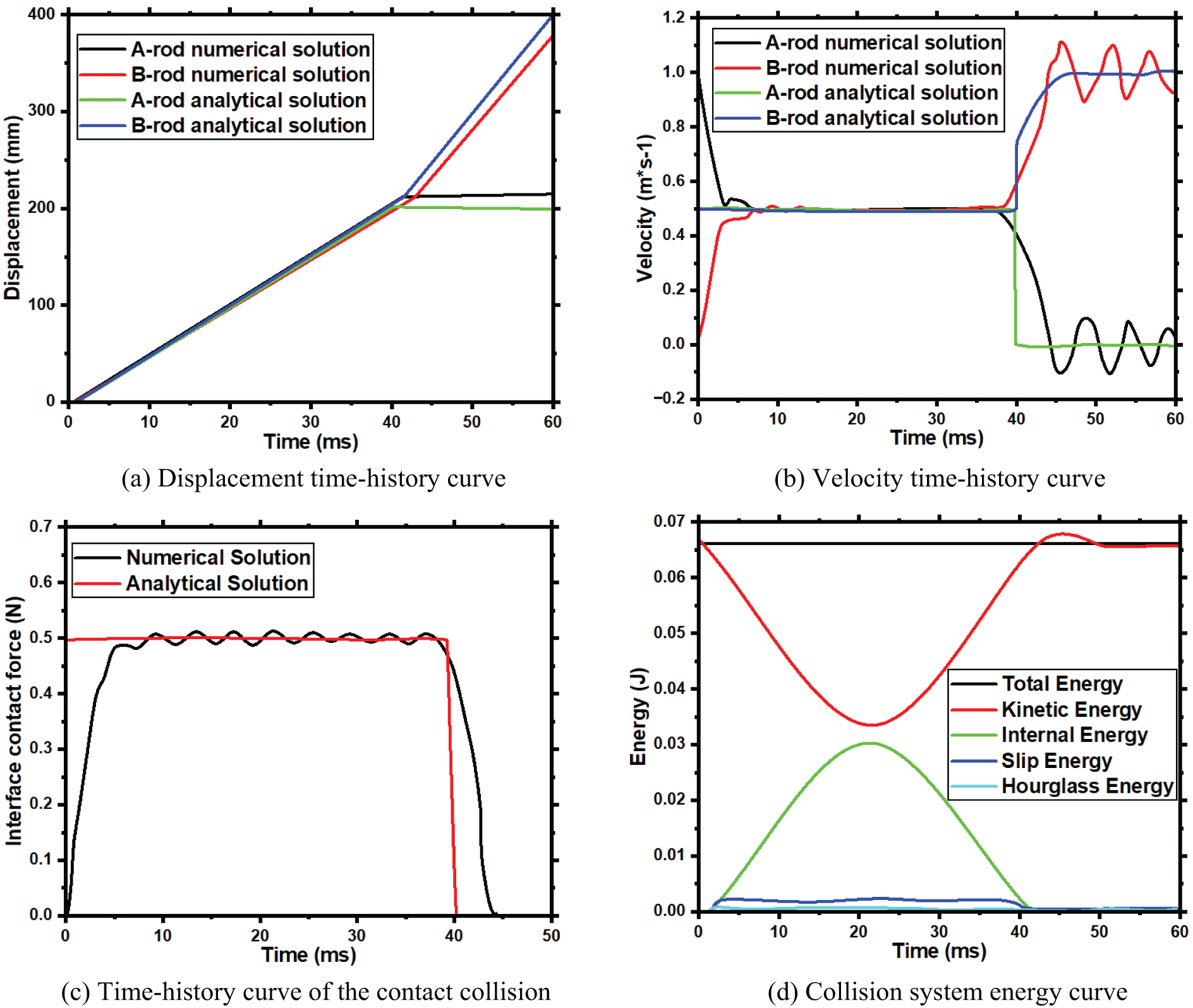
Figure 19: Outputs of the center point of the contact surface

6.4 Verification of ABAQUS

An investigation into the propagation of stress waves within Rods A and B during the impact process was conducted. These observations align with the principles of one-dimensional elastic wave theory [63,64]. The use of the ABAQUS program for analyzing this collision problem was reliable. Further examination of the computational accuracy of the ABAQUS program was conducted by comparing time-history curves of displacement, velocity, and contact force at the central nodes of the contact surfaces of Rods A and B, as well as the energy curve of the collision system, to theoretical and analytical solutions, as demonstrated in Fig. 19. The analytical contact force solution assumes an initial penetration depth per Hertzian contact theory, whereas the numerical model starts with no penetration. The analysis determined the displacement time history through the analytical resolution of the one-dimensional wave equation applied to an elastic rod under the impact. The equation for the 1D wave in an elastic rod is expressed as ∂2u/∂t2=c2 ∂2u/∂x2 , wherein u represents displacement, c is the wave speed, x is the position, and t is time. This process involved obtaining a closed-form solution for displacement as a function of time and position along the subjected rod.

To solve the wave equation, d’Alembert’s approach was employed, wherein the equilibrium equation was integrated twice concerning time and position. This method incorporated appropriate initial and boundary conditions based on the initial velocity and free rod ends. As a result, the displacement at the center of the rod, as a function of time, was determined. This solution is graphically represented in Fig. 19a. D’Alembert’s approach, which involves the double integration of the wave equation, can be mathematically represented as follows: ∫∫∂2u/∂t2 dt dx=∫∫c2 ∂2u/∂x2 dt dx . The initial conditions, u(x, 0)=0 and ∂u/∂t (x, 0)=v0 , and boundary conditions, ∂u/∂x(0, t)=0 and ∂u/∂x(L, t)=0 , were applied, and the resulting integral was analytically solved to obtain: u(x, t)=(v0/c)f(x,  ct) . Here, f(x, ct) represents the waveform function. The solution at x=L/2 provided the displacement at the center. The velocity time history was acquired by taking the first derivative of the displacement solution concerning time, yielding v(x, t)=∂u/∂t=(v0/c)∂f/∂(ct) . This process offered an analytical velocity at the rod center x=L/2 over time, as shown in Fig. 19b. The contact force solution was obtained from Hertzian contact theory for the elastic impact of two rods, expressed as F = kδ1^.5 , where F is force, δ is the penetration depth, and k is a constant. The penetration depth was determined from the displacement solution and relative velocities. The contact force F at each time step was computed based on δ and k . This analytical contact force was then plotted against the result from ABAQUS, as depicted in Fig. 19c. The initial non-zero contact force in the analytical solution results from the assumed initial penetration per Hertz theory. While the initial contact forces differ due to differing penetration assumptions, the subsequent force vs. time trends agree well between the two solutions. The collective results offered a comprehensive understanding of the displacement, velocity, and contact force behavior under the defined conditions.

6.5 Discussion

It can be seen from the above Figures that the contact surface displacement, velocity, and impact force calculated by ABAQUS during the impact process of the elastic rod are completely consistent with the theoretical and analytical solutions, and the system energy remains conserved during the elastic collision. The numerical oscillations caused by the calculation during the impact are also small. The analytical solution used a simplified case of both rods initially stationary, while the numerical model used an initial velocity of 1 m/s for Rod A, as defined in Section 6.2. In the velocity time history curve, the curve after 0.04 s oscillates greatly because the structural damping and material damping are not set in the calculation, so the initial impact stress wave in the elastic rod has been oscillating and cannot be eliminated. In Fig. 19, during the collision contact process (before 0.04 s), the displacements of the contact surfaces of the elastic Rods A and B are not the same because there is a certain amount of penetration in the contact. A certain amount of penetration is an unavoidable phenomenon of the ABAQUS Penalty Method to solve the collision problem. Reducing the amount of penetration will bring about the oscillation of the calculation, which is a pair of irreconcilable contradictions. To sum up, the calculation accuracy of ABAQUS in solving the collision problem fully meets scientific research needs.

7  Conclusion

This paper has comprehensively examined the nonlinearities in collision and impact problems, focusing on geometric nonlinearity, contact nonlinearity (nonlinear boundary conditions), and material nonlinearity. The study delved into the numerical realization process of collision and impact problems, giving a detailed analysis of the stress and strain occurring during large deformations in collisions. It also scrutinized the fundamental finite element solution methods to address these large deformation issues. Further, the research examined the hourglass mode and its control using single-point reduced integration, as well as the integration of contact-collision algorithms within the finite element framework. The paper also explored the complexities of material nonlinearity, providing an in-depth understanding of different contributing factors. To complement these theoretical explorations, the paper also expanded upon the practical applicability of these findings. Specifically, it utilized a distinct model considering steel-concrete bond slip to analyze RC members’ dynamic response behavior and failure modes under asymmetrical impact loads. It was observed that increasing the hammer’s mass and initial velocity intensified the dynamic response and damage to the RC member. Conversely, while increasing axial compressive strength did not effectively reduce horizontal displacement, enhancing longitudinal reinforcement and stirrup ratios significantly improved RC members’ anti-collision capacity. Regarding failure modes under impact load, RC members exhibited local failure primarily concrete crushing and offside spalling and overall failure, usually characterized as bending shear failure with bending deformation preceding shear deformation. The practical application of the research was further validated through an elastic rod impact case study, which analyzed the propagation of stress waves and compared ABAQUS numerical solutions with theoretical and analytical solutions for various parameters, demonstrating the reliability and accuracy of the ABAQUS program in analyzing impact problems. In conclusion, this study contributes valuable insights into the nonlinearities in collision and impact problems and provides effective strategies for enhancing the resilience of RC structures under dynamic stress. The findings advance our theoretical understanding and offer practical solutions, forming a comprehensive perspective.

Acknowledgement: Not applicable.

Funding Statement: This work was supported by the authority of the National Natural Science Foundation of China (Grant Nos. 52178168 and 51378427) for financing this research work and several ongoing research projects related to structural impact performance.

Author Contributions: The authors confirm contribution to the paper as follows: study conception and design: Khalil, Liu; data collection: Liu; analysis and interpretation of results: Khalil, Liu, Zhao; draft manuscript preparation: Khalil, Han. All authors reviewed the results and approved the final version of the manuscript.

Availability of Data and Materials: All the data that used in this paper mentioned in the content.

Conflicts of Interest: The authors declare that they have no conflicts of interest to report regarding the present study.

References

1. Kimura, K., Onogi, T., Yotsumoto, N., Ozaki, F. (2023). Bending strength of full-scale wide-flange steel beams considering strain rate effects at elevated temperatures. Journal of Structural Fire Engineering, 14(4), 598–625. [Google Scholar]

2. Wu, G. X., Taylor, R. E. (2003). The coupled finite element and boundary element analysis of nonlinear interactions between waves and bodies. Ocean Engineering, 30, 387–400. 10.1016/S0029-8018(02)00037-9. [Google Scholar]

3. Anas, S. M., Alam, M., Shariq, M. (2023). Damage response of conventionally reinforced two-way spanning concrete slab under eccentric impacting drop weight loading. Defence Technology, 19, 12–34. https://doi.org/10.1016/j.dt.2022.04.011. [Google Scholar]

4. Anas, S. M., Shariq, M., Alam, M., Yosri, A. M., Mohamed, A. et al. (2023). Influence of supports on the Low-velocity impact response of square RC slab of standard concrete and ultra-high-performance concrete: FEM-based computational analysis. Buildings, 13(5), 1220. [Google Scholar]

5. Kane, C., Repetto, E. A., Ortiz, M., Marsden, J. E. (1999). Finite element analysis of nonsmooth contact. Computer Methods in Applied Mechanics and Engineering, 180, 1–26. https://doi.org/10.1016/S0045-7825(99)00034-1. [Google Scholar]

6. Eberhard, P. (1999). Collision detection and contact approaches for a hybrid multibody system/finite element simulation. IUTAM Symposium on Unilateral Multibody Contacts, 72, 193–202. https://doi.org/10.1007/978-94-011-4275-5. [Google Scholar]

7. Gantes, C. J. (2014). Nonlinear finite element analysis. Encyclopedia of Earthquake Engineering, 1, 1–35. [Google Scholar]

8. Krysko, A. V., Awrejcewicz, J., Saltykova, O. A., Vetsel, S. S., Krysko, V. A. (2016). Nonlinear dynamics and contact interactions of the structures composed of beam-beam and beam-closed cylindrical shell members. Chaos Solitons Fractals, 91, 622–638. https://doi.org/10.1016/j.chaos.2016.09.001. [Google Scholar]

9. He, Z. F., Jia, N., Wang, H. W., Liu, Y., Li, D. Y. et al. (2020). The effect of strain rate on mechanical properties and microstructure of a metastable FeMnCoCr high entropy alloy. Materials Science and Engineering: A, 776, 138982. https://doi.org/10.1016/j.msea.2020.138982. [Google Scholar]

10. Mishra, S. K., Roy, H., Dutta, K. (2018). Influence of ratcheting strain on tensile properties of A356 alloy. Materials Today: Proceedings, 5, 12403–12408. [Google Scholar]

11. Bayazit, O. B., Lien, J. M., Amato, N. M. (2002). Probabilistic roadmap motion planning for deformable objects. Proceedings-IEEE International Conference on Robotics and Automation, vol. 2, pp. 2126–2133. Washington DC, USA. [Google Scholar]

12. Shinya, M., Fournier, A. (1992). Stochastic motion—Motion under the influence of wind. Computer Graphics Forum, 11, 119–128. https://doi.org/10.1111/cgf.1992.11.issue-3. [Google Scholar]

13. Long, D., Viovy, J. L., Ajdari, A. (1996). Simultaneous action of electric fields and nonelectric forces on a polyelectrolyte: Motion and deformation. Physical Review Letters, 76, 3858. https://doi.org/10.1103/PhysRevLett.76.3858. [Google Scholar] [PubMed]

14. Christensen, G. E., Rabbitt, R. D., Miller, M. I. (1996). Deformable templates using large deformation kinematics. IEEE Transactions on Image Processing, 5, 1435–1447. https://doi.org/10.1109/83.536892. [Google Scholar] [PubMed]

15. Laursen, T. A., Simo, J. C. (1993). A continuum-based finite element formulation for the implicit solution of multibody, large deformation-frictional contact problems. International Journal for Numerical Methods in Engineering, 36, 3451–3485. https://doi.org/10.1002/nme.v36:20. [Google Scholar]

16. Chen, Y. C., Lagoudas, D. C. (2008). A constitutive theory for shape memory polymers. Part I: Large deformations. Journal of the Mechanics and Physics of Solids, 56, 1752–1765. https://doi.org/10.1016/j.jmps.2007.12.005. [Google Scholar]

17. Schlenker, J. L., Gibbs G, V., Boisen, M. B. (1978). Strain-tensor components expressed in terms of lattice parameters. Acta Crystallographica Section A, 34, 52–54. https://doi.org/10.1107/S0567739478000108. [Google Scholar]

18. Santarpia, E., Demasi, L. (2020). Large displacement models for composites based on Murakami’s Zig-Zag function, green-lagrange strain tensor, and generalized unified formulation. Thin-Walled Structures, 150, 106460. https://doi.org/10.1016/j.tws.2019.106460. [Google Scholar]

19. Gullett, P. M., Horstemeyer, M. F., Baskes, M. I., Fang, H. (2007). A deformation gradient tensor and strain tensors for atomistic simulations. Modelling and Simulation in Materials Science and Engineering, 16, 015001. [Google Scholar]

20. Hackett, R. M. (2018). Stress measures. In: Hyperelasticity primer, pp. 29–48. Cham, Germany: Springer. [Google Scholar]

21. Kulikov, G. M., Plotnikova, S. V. (2019). Analysis of the second Piola-Kirchhoff stress in nonlinear thick and thin structures using exact geometry SaS solid-shell elements. International Journal for Numerical Methods in Engineering, 117, 498–522. https://doi.org/10.1002/nme.v117.5. [Google Scholar]

22. Cao, T., Cuffari, D., Bongiorno, A. (2018). First-principles calculation of third-order elastic constants via numerical differentiation of the second Piola-Kirchhoff stress tensor. Physical Review Letter, 121, 216001. https://doi.org/10.1103/PhysRevLett.121.216001. [Google Scholar]

23. Dienes, J. K. (1987). A discussion of material rotation and stress rate. Acta Mechanica, 65, 1–11. https://doi.org/10.1007/BF01176868. [Google Scholar]

24. Flanagan, D. P., Taylor, L. M. (1987). An accurate numerical algorithm for stress integration with finite rotations. Computer Methods in Applied Mechanics and Engineering, 62, 305–320. https://doi.org/10.1016/0045-7825(87)90065-X. [Google Scholar]

25. Gambirasio, L., Chiantoni, G., Rizzi, E. (2016). On the consequences of the adoption of the Zaremba–Jaumann objective stress rate in FEM codes. Archives of Computational Methods in Engineering, 23, 39–67. https://doi.org/10.1007/s11831-014-9130-z. [Google Scholar]

26. Harko, T. (2014). Thermodynamic interpretation of the generalized gravity models with geometry-matter coupling. Physical Review D, 90, 044067. https://doi.org/10.1103/PhysRevD.90.044067. [Google Scholar]

27. Cho, K. S. (2021). Energy-conserving DPD and thermodynamically consistent Fokker–Planck equation. Physica A: Statistical Mechanics and its Applications, 583, 126285. https://doi.org/10.1016/j.physa.2021.126285. [Google Scholar]

28. He, X., Doolen, G. D. (2002). Thermodynamic foundations of kinetic theory and Lattice Boltzmann models for multiphase flows. Journal of Statistical Physics, 107, 309–328. https://doi.org/10.1023/A:1014527108336. [Google Scholar]

29. Léger, S., Fortin, A., Tibirna, C., Fortin, M. (2014). An updated Lagrangian method with error estimation and adaptive remeshing for very large deformation elasticity problems. International Journal for Numerical Methods in Engineering, 100, 1006–1030. https://doi.org/10.1002/nme.v100.13. [Google Scholar]

30. Yang, Y. B., Lin, S. P., Leu, L. J. (2007). Solution strategy and rigid element for nonlinear analysis of elastically structures based on updated Lagrangian formulation. Engineering Structures, 29, 1189–1200. https://doi.org/10.1016/j.engstruct.2006.08.015. [Google Scholar]

31. Wessels, H., Weißenfels, C., Wriggers, P. (2020). The neural particle method–an updated Lagrangian physics informed neural network for computational fluid dynamics. Computer Methods in Applied Mechanics and Engineering, 368, 113127. https://doi.org/10.1016/j.cma.2020.113127. [Google Scholar]

32. Database, C. M., Session, S., Tutorial, A. et al. (2014). Abaqus/CAE 6.14 user’s manual. RI, USA: Dassault Systémes Inc. Providence. [Google Scholar]

33. Chaudhari, V. S. , Chakrabarti, A. M. (2012). Modeling of concrete for nonlinear analysis using finite element code ABAQUS. International Journal of Computer Applications, 44(7), 14–18. [Google Scholar]

34. Seo, H., Hundley, J., Hahn, H. T., Yang, J. M. (2012). Numerical simulation of glass-fiber-reinforced aluminum laminates with diverse impact damage. AIAA Journal, 48(3), 676–687. [Google Scholar]

35. Scovazzi, G. (2012). Lagrangian shock hydrodynamics on tetrahedral meshes: A stable and accurate variational multiscale approach. Journal of Computational Physics, 231:8029–8069. https://doi.org/10.1016/j.jcp.2012.06.033. [Google Scholar]

36. Koudelka Supervisor, P., Ing Ondřej Jiroušek, P. (2020). Numerical modelling of auxetic structures. Acta Polytechnica CTU Proceeding, 18, 38–43. [Google Scholar]

37. Bloxom, A. L. (2014). Numerical simulation of the fluid-structure interaction of a surface effect ship bow seal. USA: Virginia Polytechnic Institute and State University. [Google Scholar]

38. Wu, S. W., Wan, D. T., Jiang, C., Liu, X., Liu, K. et al. (2023). A finite strain model for multi-material, multi-component biomechanical analysis with total Lagrangian smoothed finite element method. International Journal of Mechanical Sciences, 243, 108017. https://doi.org/10.1016/j.ijmecsci.2022.108017. [Google Scholar]

39. Mendes, N., Nochebuena-Mora, E., Lourenço, P. B. (2023). Numerical application of viscoelastic devices for improving the out-of-plane behaviour of a historic masonry building. Lecture Notes in Civil Engineering, 309, 575–585. https://doi.org/10.1007/978-3-031-21187-4. [Google Scholar]

40. Nguyen, T. N., Eatherton, M. R. (2023). Computational and experimental study of structural fuses optimized to resist buckling. Journal of Constructional Steel Research, 201, 107688. https://doi.org/10.1016/j.jcsr.2022.107688. [Google Scholar]

41. Zhai, S. Y., Lyu, Y. F., Cao, K., Li, G. Q., Wang, W. Y. et al. (2023). Seismic behavior of an innovative bolted connection with dual-slot hole for modular steel buildings. Engineering Structures, 279, 115619. https://doi.org/10.1016/j.engstruct.2023.115619. [Google Scholar]

42. Zhang, P., Du, C., Tian, X., Jiang, S. (2018). A scaled boundary finite element method for modelling crack face contact problems. Computer Methods in Applied Mechanics and Engineering, 328, 431–451. https://doi.org/10.1016/j.cma.2017.09.009. [Google Scholar]

43. Abdel Wahab, M. M., de Roeck, G., Peeters, B. (1999). Parameterization of damage in reinforced concrete structures using model updating. Journal of Sound and Vibration, 228, 717–730. https://doi.org/10.1006/jsvi.1999.2448. [Google Scholar]

44. Lei, Z., Zang, M. (2010). An approach to combining 3D discrete and finite element methods based on penalty function method. Computational Mechanics, 46, 609–619. https://doi.org/10.1007/s00466-010-0502-4. [Google Scholar]

45. Fan, W., Zhong, Z., Huang, X., Sun, W., Mao, W. (2022). Multi-platform simulation of reinforced concrete structures under impact loading. Engineering Structures, 266, 114523. https://doi.org/10.1016/j.engstruct.2022.114523. [Google Scholar]

46. Abbas, N., Yousaf, M., Akbar, M., Saeed, M. A., Huali, P. et al. (2022). An experimental investigation and computer modeling of direct tension pullout test of reinforced concrete cylinder. Inventions, 7, 77. https://doi.org/10.3390/inventions7030077. [Google Scholar]

47. Shu, Y., Wang, G., Lu, W., Chen, M., Lv, L. et al. (2022). Damage characteristics and failure modes of concrete gravity dams subjected to penetration and explosion. Engineering Failure Analysis, 134, 106030. https://doi.org/10.1016/j.engfailanal.2022.106030. [Google Scholar]

48. Abaqus/CAE (2019). https://www.3ds.com/edu/education/students/solutions/abaqus-le (accessed on 07/03/2024). [Google Scholar]

49. Yao, S., Zhang, D., Lu, F., Wang, W., Chen, X. (2016). Damage features and dynamic response of RC beams under blast. Engineering Failure Analysis, 62, 103–111. https://doi.org/10.1016/j.engfailanal.2015.12.001. [Google Scholar]

50. Hsiao, H. M., Daniel, I. M. (1998). Strain rate behavior of composite materials. Composites Part B: Engineering, 29, 521–533. https://doi.org/10.1016/S1359-8368(98)00008-0. [Google Scholar]

51. Hibbitt, D., Karlsson, B., Sorensen, P. (2010). ABAQUS 6.10 analysis user’s manual, vol. 8. Pawtucket, USA: Engineering. [Google Scholar]

52. Al-Bukhaiti, K., Liu, Y. H., Zhao, S. C., Abas, H. (2022). Dynamic simulation of CFRP-shear strengthening on existing square RC members under unequal lateral impact loading. Structural Concrete, 24, 1572–1596. [Google Scholar]

53. AL-Bukhaiti, Liu, Y. H., Zhao, S. C., Abas, H., Yu, Y. X. et al. (2023). Failure mechanism and static bearing capacity on circular RC members under asymmetrical lateral impact train collision. Structures, 48, 1817–1832. https://doi.org/10.1016/j.istruc.2023.01.075. [Google Scholar]

54. Yanhui, L., Al-Bukhaiti, K., Shichun, Z., Abas, H., Nan, X. et al. (2022). Numerical study on existing RC circular section members under unequal impact collision. Scientific Reports, 12, 14793. https://doi.org/10.1038/s41598-022-19144-1. [Google Scholar] [PubMed]

55. Le Minh, H., Khatir, S., Abdel Wahab, M., Cuong-Le, T. (2021). A concrete damage plasticity model for predicting the effects of compressive high-strength concrete under static and dynamic loads. Journal of Building Engineering, 44, 103239. https://doi.org/10.1016/j.jobe.2021.103239. [Google Scholar]

56. AL-Bukhaiti, K., Yanhui, L. (2023). Effect of the axial load on the dynamic response of the wrapped CFRP reinforced concrete column under the asymmetrical lateral impact load. PLoS One, 18, 1–30. [Google Scholar]

57. Duenser, S., Poranne, R., Thomaszewski, B., Coros, S. (2020). RoboCut. ACM Transactions on Graphics. https://doi.org/10.1145/3386569.3392465 [Google Scholar] [CrossRef]

58. Guo, Y., Yin, X., Yu, B., Hao, Q., Xiao, X. et al. (2023). Experimental analysis of dynamic behavior of elastic visco-plastic beam under repeated mass impacts. International Journal of Impact Engineering, 171, 104371. https://doi.org/10.1016/j.ijimpeng.2022.104371. [Google Scholar]

59. Sintov, A., Macenski, S., Borum, A., Bretl, T. (2020). Motion planning for dual-arm manipulation of elastic rods. IEEE Robot Autom Letter, 5, 6065–6072. https://doi.org/10.1109/LSP.2016. [Google Scholar]

60. Choi, A., Tong, D., Jawed, M. K., Joo, J. (2021). Implicit contact model for discrete elastic rods in knot tying. Journal of Applied Mechanics, Transactions, 88, 051010-10. [Google Scholar]

61. Lv, N., Liu, J., Jia, Y. (2022). Dynamic modeling and control of deformable linear objects for single-arm and dual-arm robot manipulations. IEEE Transactions on Robotics, 38, 2341–2353. https://doi.org/10.1109/TRO.2021.3139838. [Google Scholar]

62. Yin, S., Chen, D., Xu, J. (2019). Novel propagation behavior of impact stress wave in one-dimensional hollow spherical structures. International Journal of Impact Engineering, 134, 103368. https://doi.org/10.1016/j.ijimpeng.2019.103368. [Google Scholar]

63. Bednarik, M., Cervenka, M., Groby, J. P., Lotton, P. (2018). One-dimensional propagation of longitudinal elastic waves through functionally graded materials. International Journal of Solids Structures, 146, 43–54. https://doi.org/10.1016/j.ijsolstr.2018.03.017. [Google Scholar]

64. Mirzajani, M., Khaji, N., Hori, M. (2018). Stress wave propagation analysis in one-dimensional micropolar rods with variable cross-section using micropolar wave finite element method. International Journal of Applied Mechanics, 10(4), 1850039. [Google Scholar]