 Open Access
ARTICLE
Predicting Reliability and Remaining Useful Life of Rolling Bearings Based on Optimized Neural Networks
School of Automation and Electrical Engineering, Dalian Jiaotong University, Dalian, 116028, China
* Corresponding Author: Tiantian Liang. Email:
Structural Durability & Health Monitoring 2023, 17(5), 433-455. https://doi.org/10.32604/sdhm.2023.029331
Received 13 February 2023; Accepted 13 April 2023; Issue published 07 September 2023
Abstract
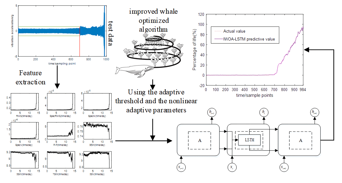
In this study, an optimized long short-term memory (LSTM) network is proposed to predict the reliability and remaining useful life (RUL) of rolling bearings based on an improved whale-optimized algorithm (IWOA). The multi-domain features are extracted to construct the feature dataset because the single-domain features are difficult to characterize the performance degeneration of the rolling bearing. To provide covariates for reliability assessment, a kernel principal component analysis is used to reduce the dimensionality of the features. A Weibull distribution proportional hazard model (WPHM) is used for the reliability assessment of rolling bearing, and a beluga whale optimization (BWO) algorithm is combined with maximum likelihood estimation (MLE) to improve the estimation accuracy of the model parameters of the WPHM, which provides the data basis for predicting reliability. Considering the possible gradient explosion by training the rolling bearing lifetime data and the difficulties in selecting the key network parameters, an optimized LSTM network called the improved whale optimization algorithm-based long short-term memory (IWOA-LSTM) network is proposed. As IWOA better jumps out of the local optimization, the fitting and prediction accuracies of the network are correspondingly improved. The experimental results show that compared with the whale optimization algorithm-based long short-term memory (WOA-LSTM) network, the reliability prediction and RUL prediction accuracies of the rolling bearing are improved by the proposed IWOA-LSTM network.Graphic Abstract
Keywords
With advances in technology, the precision and complexity of various mechanical devices are increasing. As an indispensable basic component of mechanical devices, rolling bearings directly determine the safety and reliability of mechanical devices [1]. When high-strength wear, fracture, and failure occur, the device must often be stopped for maintenance, which can cause serious accidents and casualties [2]. Thus, based on vibration signals, it is important to improve the performance of rolling bearings to avoid catastrophic accidents by implementing a reliability assessment and remaining useful life (RUL) prediction for rolling bearings before faults occur [3].
Theoretical and experimental studies have shown that data-driven methods have become the main methods for reliability prediction and RUL prediction [4,5]. The concrete implementation can be summarized as follows. Based on vibration signals, multidimensional data reflecting degeneration feature trends are extracted. Then, the neural networks are constructed and trained so that reliability prediction and RUL prediction are implemented. Generally, multidomain features include the features of the time, frequency, and time–frequency domains. Investigations have been conducted on feature extraction. To address the insufficient feature vectors, the features of the time and frequency domains were extracted [6]; however, the time–frequency domain features were ignored. Some researchers have focused on time–frequency domain feature extraction of vibration signals based on the empirical mode decomposition (EMD) method [7–9]. However, it is well known that endpoint effects and modal component mixing of EMD exist [10]. Thus, variational mode decomposition (VMD) has been combined with wavelet transform to extract the time–frequency domain features [11]. The periodic features of every IMF are more obvious owing to the VMD, and the prediction performance has improved. However, these methods extracted only single-domain features, and complete feature information was not collected. Although the degeneration features of the time, frequency, and time–frequency domains have been extracted to implement the RUL prediction of the rolling bearing [12], the feature extraction of the time–frequency domain has remained an EMD-based method that requires further improvement.
In the stage of product testing, reliability assessment and prediction usually play an important role in product quality management [13]. For the reliability assessment, the Weibull distribution proportional hazard model (WPHM) was constructed and applied to the reliability evaluation of bearings based on the Weibull function [14]. Moreover, a Bayesian network was used for the weighted fusion of features combined with a proportional hazard model to implement a reliability assessment [15]. Because the accuracy of the reliability evaluation model depends on the values of its parameters, the parameter estimation method needs to be studied emphatically. Based on modified maximum likelihood estimation (MLE), the parameter estimation of the reliability model has been implemented [16]. Particle swarm optimization (PSO) was combined with MLE to improve parameter estimation accuracy [17]. However, this accuracy still needs to be improved because the PSO is easy to trap into the local optimum. Reliability prediction was implemented using a relevance vector machine (RVM) [18]. However, the randomness of the parameters in the RVM may lead to a large reliability assessment error. By combining the Bayesian optimization algorithm (BOA) with the mixed kernel RVM (MKRVM), the reliability assessment and prediction accuracy of the rolling bearing were improved [19]. From the above investigations, it is clear that constructing a suitable reliability model and a reliability assessment method is important for reliability prediction.
Additionally, RUL prediction is an important topic, that is, predicting the failure time of rolling bearings in the future and the probability of failure. With the development of deep learning and improvement in optimization algorithms, optimized deep recurrent neural networks have been used for time series prediction, and many prominent results have been reported in recent years. Based on the PSO algorithm, the back propagation neural network (BPNN) has been optimized and has obtained better robustness and prediction accuracy [20]. Based on improved gray wolf optimization, the radial basis function neural network (RBFNN) was optimized [21]. However, owing to the structure of the RBFNN, it may lead to gradient vanishing and gradient explosion, which are inapplicable for predicting time series information over a long time. Thus, a long short-term memory (LSTM) network has been designed, and many optimization algorithms have been used to improve the performance of the LSTM network. To improve the prediction accuracy of the network, a differential evolution algorithm was proposed to optimize the LSTM network [22]. A gray wolf optimizer (GWO) was combined with the LSTM network to demonstrate the excellent convergence of the network. However, the training time of the network increases with the iteration of the GWO because of its complex characteristics [23]. An improved PSO (IPSO) algorithm was proposed to search for the parameters of the LSTM network, but the operating time of the network increased as the calculation of the IPSO increased [24]. The WOA was used to optimize the learning rate and iterations of the LSTM network [25]. However, the performance of the WOA requires further improvement, because it can be easily trapped into local optimization.
For these reasons, this study proposes an optimized LSTM network to implement better reliability prediction and RUL prediction. First, based on the entire life data of the rolling bearing, the features of the time, frequency, and time–frequency domains are extracted, and a feature dataset is constructed. Then, to obtain the covariates, kernel principal component analysis (KPCA) is utilized to reduce the dimensions of the feature dataset. Based on these covariates, a WPHM is constructed for the reliability assessment, and a beluga whale optimization (BWO) algorithm is introduced to optimize the MLE for the parameter estimation of the WPHM; therefore, the reliability assessment accuracy is further improved. Furthermore, based on the adaptive threshold and nonlinear adaptive weights, an improved whale-optimized algorithm (IWOA) is proposed to better jump out of the local optimization, and an IWOA-LSTM network is constructed. By combining the reliability assessment data obtained by the WPHM with the improved whale optimization algorithm-based long short-term memory (IWOA-LSTM) network, the reliability prediction and RUL prediction of the rolling bearings are better implemented because IWOA better avoids randomness by applying the manual section of the key parameters of the LSTM network.
The rest of this paper is organized as follows. In Section 2, based on the experimental data and feature extraction methods, a feature dataset is constructed for the entire life vibration signal of rolling bearings. In Section 3, the kernel principal component analysis (KPCA) algorithm is used to reduce the dimension of the extracted feature dataset, and the MLE is optimized using the BWO algorithm to improve the estimation accuracy of the unknown parameters of the WPHM model, which evaluates the reliability of the bearing. In Section 4, an IWOA is proposed based on the adaptive threshold and nonlinear adaptive weights to optimize the key parameters of the LSTM network so that reliability prediction and RUL prediction can be implemented. In Section 5, the experimental results are presented, and the prediction results obtained by the IWOA-LSTM network are compared with those of previous studies to show the effectiveness of the proposed method. Finally, conclusions are presented in Section 6.
In this study, the rolling bearing life cycle experimental data [26] are presented, and a diagram of the life cycle experiment platform is shown in Fig. 1. Moreover, the sampled frequency of the experiment is 20 kHz, and the sampled points are 20480, as shown in Table 1.
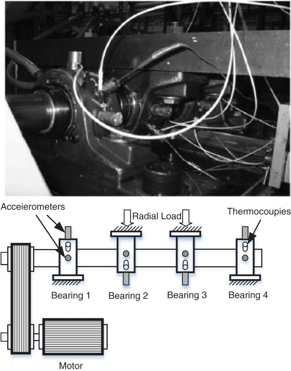
Figure 1: Diagram of the experimental platform

During the three groups of experiments, owing to the various failure conditions of the rolling bearing, some bearings were still in the stage of intermediate fault or even incipient fault at the end of the experiments. Thus, the life features of these bearings are inapplicable to this investigation. After comparison, the degenerate data of bearing 1 of experiment 2, in which the outer ring failure occurs, are selected as the test data. The data of bearings 3 and 4 of experiment 1 as well as the data of bearing 3 of experiment 3 are selected as the training data in this study.
A major effective method for reliability prediction and RUL prediction is vibration signal analysis. In this study, the vibration signal features of time, frequency, and the time–frequency domains are all considered and extracted for further screening of the feature parameters that reflect the effective degeneration.
First, consider the feature parameter extraction of the time domain. Typically, the time-domain information for feature extraction of the vibration signals includes the mean value, root mean square (RMS), peak, peak-to-peak (P-P), kurtosis value, peak factor, shape factor, and margin factor.
Then, consider the feature parameter extraction of the frequency domain. Generally, analysis in the time domain is more intuitive, while representation in the frequency domain is more concise. These two analytical methods are interrelated and complementary. The vibration signals in the time domain are transformed into the frequency domain so that the spectral data are arranged in the time dimension, which also exhibits a degenerate trend. Thus, for an aperiodic signal
and the multifrequency domain feature parameters, such as the frequency domain RMS, frequency variance, and frequency mean, are extracted from the transformed signal.
Finally, consider the feature parameter extraction in the time–frequency domain. To analyze the law of nonstationary signal spectrum changes with time, two analysis methods are presented in this study considering that different types of features depend on different analysis methods.
The first feature parameter extraction method in the time–frequency domain is chosen as the wavelet transform because it has variable time and frequency windows, that is, higher time resolution at high frequencies and higher frequency resolution at lower frequencies, enabling it to characterize the rolling bearing degradation trends.
The specific formula of the wavelet transform is expressed as follows:
where
The second feature parameter extraction method in the time–frequency domain is chosen as VMD. Traditional EMD has an endpoint effect and modal component mixing, which requires improvement. Thus, as an adaptive and fully nonrecursive method for modal variation and signal processing, VMD is proposed to better process the signal. VMD reduces the nonstationarity of time series with high complexity and strong nonlinearity and decomposes them to obtain relatively stationary subsequences containing multiple different frequency scales. For these reasons, the penalty factor and the number of modal components in the VMD are optimized by the PSO, and the energy characteristics of the decomposed signal of the VMD are extracted in this study. The energy values of the third and seventh frequency bands are chosen as the features.
Using the above data source and analyzing the variation signals, multiple feature parameters are extracted from the time, frequency, and time–frequency domains. Among these, time-domain feature parameters are extracted as the mean, RMS, peak, and peak factors. Frequency domain feature parameters, such as spectrum amplitude, power spectrum amplitude, and cepstrum, are extracted. The extracted time–frequency domain feature parameters include the wavelet packet, energy entropy, and sample entropy of each frequency band decomposed by the VMD. Excluding the features with insignificant monotonic change in the main trend and those that exhibit similar functions or meanings but reflect poor relative effects of the performance degradation process, 14 features of time, frequency, and time–frequency domains are fitted and constructed as the feature dataset. Among these, the time domain features include RMS, P-P, and the peak factor. The frequency domain features include spectrum root mean square (SpecRMS), spectrum magnitude (SpecM), and spectrum variance (SpecV). The time–frequency domain features include the 3rd frequency band energy spectrum of the wavelet packet (3SW), the 7th frequency band energy spectrum of the wavelet packet (7SW), the 3rd frequency band sample entropy of the wavelet packet (3EW), the 7th frequency band sample entropy of the wavelet packet (7EW), the 3rd frequency band energy spectrum of the VMD (3SV), the 7th frequency band energy spectrum of the VMD (7SV), the 3rd frequency band sample entropy of the VMD (3EV), and the 7th frequency band sample entropy of the VMD (7EV).
3 Reliability Assessment of Rolling Bearing
In this section, a reliability assessment is implemented based on the KPCA. Moreover, a BWO is utilized to optimize the MLE, and a BWO-MLE is proposed. WPHM is established based on a more accurate parameter estimation using the BWO-MLE, which provides a data basis for the reliability prediction, and is presented as one of the features for the RUL prediction.
The KPCA is the nonlinear extension of the PCA. Owing to the characteristics of the Gaussian kernel function, such as few parameters and simple calculation processes, it is chosen as the kernel function of nonlinear mapping. The derivation process of the KPCA is summarized as follows.
The Gaussian function maps each feature vector
where
where
Then, the inner product of
The eigenvector V is linearly expressed as follows:
where
where
The projection of x on
In this study, owing to its excellent robustness, flexibility, and good fit to the failure rate curve of the WPHM device, it is selected to describe the failure risk degree of the rolling bearing degradation process. Based on the WPHM, the failure rate and reliability function are established, which are further used for the reliability prediction and RUL prediction of the rolling bearing during the entire life process. The failure rate of the WPHM is expressed as follows:
where
and the reliability function is obtained as
The selection of unknown parameters in the reliability model significantly affects the results of reliability evaluation. In this subsection, the kernel principal component obtained after dimension reduction by KPCA is chosen as the covariate, and BWO [27] is utilized to optimize the MLE for a more accurate parameter estimation of the WPHM model. The main principle of the BWO algorithm is as follows.
The location matrix of the search agent is modeled as follows:
where n denotes the population size of the beluga whale and d denotes the dimension of the design variable. For all belugas, the fitness values are stored in the following form:
There is a balance factor
where
(1) The exploration phase: In this phase, beluga whales are randomly selected to ensure the global search ability of the algorithm in space. Because beluga whales often swim in pairs in mirrored or synchronized poses, the position update during the exploration phase is defined as follows:
where
(2) The development phase: At this stage, the control algorithm performs a local search within the space, treats the beluga as a search agent, and directs it to move in the space by changing the position vector. The beluga preys by sharing the position information of each other, and its expression is as follows:
where
where
(3) Whale fall stage: The possibility of a whale falling is considered in the algorithm. To simulate the behavior of a whale falling in each iteration, we choose the probability of a whale falling from individuals in the population as our subjective hypothesis, thus simulating small changes in the population.
In reality, beluga whales also exhibit death or an outlier phenomenon, assuming that there is a certain probability of beluga whales in the algorithm, so there is a whale fall stage. To keep the population size unchanged, the updated position is established using the position of the beluga whale and the whale fall step length. It is expressed as follows:
where
where
The probability of whale fall decreased from 0.1 in the initial iteration to 0.05 in the last iteration, indicating that the closer the beluga was to the food source, the less dangerous the beluga was.
The optimization steps of the BWO algorithm are as follows:
Step 1. Initialize parameters, including the population size and maximum number of iterations.
Step 2. Based on the balance factor, determine how to perform the location update in different ways.
Step 3. The probability of a whale fall is calculated in each iteration, and the position is updated based on the whale fall probability.
Step 4. If the current iteration number is greater than the maximum iteration number, the BWO algorithm stops. Otherwise, the steps are repeated from Step 2.
The parameter estimation process of the MLE is as follows:
In the WPHM model, the covariates are known, and the unknown variables
where n denotes the total number of data samples, q denotes the number of sample failures, and
Then, substituting Eq. (24) into Eq. (23), the likelihood function of the WPHM model is obtained as follows:
By taking the logarithm of both sides of Eq. (25), the log-likelihood function is obtained as follows:
For the unknown parameters in Eq. (26), their partial derivatives are calculated. Then, each partial derivative is equated to zero, and a nonlinear equation system is obtained. Furthermore, the equation system is solved; then, the parameters to be estimated are obtained.
According to the value of the log-likelihood function in Eq. (26), the BWO algorithm is used to optimize the parameter estimation value of the MLE. The smaller the log-likelihood value, the higher the accuracy of the parameter estimation.
Based on the KPCA and WPHM, the steps of the proposed reliability assessment method are as follows:
Step 1. Select the feature parameters. Extract the feature parameters of time, frequency, and time–frequency domains, and the ones that can reflect the rolling bearing degradation trend are chosen to construct the feature dataset.
Step 2. Reduce the feature dimension. Use the KPCA to analyze the feature parameters, and select the kernel principal component with a cumulative contribution rate higher than 80% as a covariate.
Step 3. Construct the WPHM. Based on the MLE, the parameters of the model are estimated. To find the best parameter estimation, the BWO algorithm is used to optimize the log-likelihood value of the MLE. Then, the WPHM is constructed using the optimal parameters.
Step 4. Assess the reliability. Substitute the monitoring data into the WPHM, and calculate the cumulative failure rate and reliability of the rolling bearing. Then, the reliability curve is obtained as the basis for reliability prediction and is one of the features for RUL prediction.
4 Reliability Prediction and RUL Prediction Based on the IWOA-LSTM Network
In general, the key parameters of the LSTM network are random and difficult to select manually, which may lead to low network accuracy. Therefore, it is necessary to optimize the key parameters of the network. Some optimization algorithms have been proposed for optimizing the parameters of LSTM networks [23–25]. However, these algorithms easily fall into local optimization. Thus, to improve the ability of the WOA to jump out of the local optimization, an IWOA is proposed based on an adaptive threshold and nonlinear adaptive weights; therefore, the key parameters of the LSTM network are optimized. In this way, the prediction accuracy of the LSTM network is improved.
LSTM networks are widely used to predict long-time series events because they prevent gradient explosion by introducing a module with a memory function into the structure. The updating of the state of the cell of the LSTM network is expressed as follows:
where
The output of the memory block of the LSTM network is expressed as follows:
Although BWO exhibits excellent estimation accuracy for single-objective optimization, it may not be suitable for multi-objective optimization of the hyperparameters in the LSTM network. Moreover, the performance of the WOA for multiobjective optimization requires further improvement. Thus, an IWOA is proposed to improve the key parameters of the LSTM network.
First, the steps of the WOA are presented as follows:
Step 1. After initialization, the process of search agent update is expressed as follows:
where t denotes the current iteration,
respectively, where
Step 2. Reduce the fluctuation range of
When
where
When
Step 3. Optimize the WOA. There are two types used for optimizing the WOA
where whales choose to shrink around or spiral up depending on
Step 4. Set termination criteria to terminate the WOA.
Based on Eq. (32), the probability of each optimization method is set to 50%, and
During the iterations of the WOA, the above equal probability strategy selection may lead to inappropriate optimization for whales. Consequently, the WOA tends to have a low convergence speed and is easily trapped in local optimization. Thus, adaptive parameters are introduced to replace the original probability threshold. The introduced adaptive threshold varies from 0 to 1 with the iteration change in the WOA; therefore, whales have a greater probability of choosing a predatory strategy that is suitable for the current population in various periods. In this way, the global exploration and local development capability of the WOA are coordinated, and the convergence speed of the WOA is improved. The expression of the adaptive threshold is given as follows:
where t denotes the current iteration,
Eq. (34) implies that at the beginning of the iteration, the adaptive threshold is relatively large, which provides a greater probability for whales to implement the contraction encircle mechanism. Then, at a later stage of the iteration, the adaptive threshold becomes smaller, which gives a larger probability of implementing a spiral updating position. Based on Eq. (34), switching between either a spiral or circular movement is transformed into first contraction encircling and then spiraling up to update the position, which enhances the optimizing ability and convergence speed of the WOA.
Additionally, Eqs. (29)–(31) imply that in the position update process of the WOA, in addition to the optimizing threshold, factors that affect whales to update their position also include
where
When
The algorithm flow of the IWOA is shown in Fig. 2.
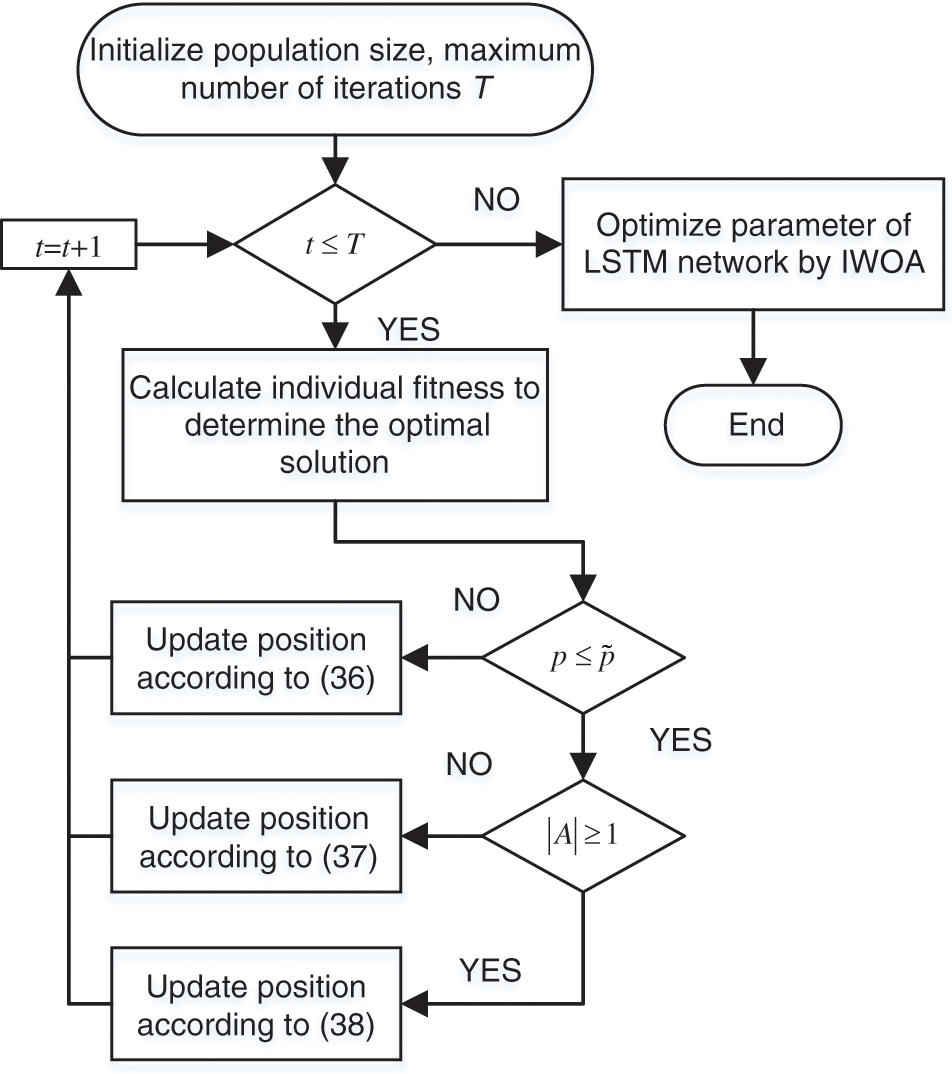
Figure 2: Algorithm flow of the IWOA
Based on the above discussion, the number of neurons in the hidden layer of the LSTM network determines the fitting ability of the model, and the number of iterations and learning rate determine the training effect. However, these parameters are difficult to determine, and the setting of the parameters usually depends on experience, which results in greater randomness. Using the proposed IWOA to optimize the parameters of the LSTM network, the randomness caused by manual selection is effectively avoided; therefore, the prediction accuracy of the LSTM network is improved. The flows of the reliability prediction and RUL prediction of the rolling bearing based on the IWOA-LSTM network are shown in Fig. 3.
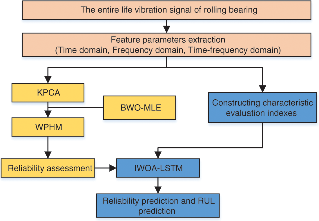
Figure 3: The flow of the reliability prediction and RUL prediction of the rolling bearing
5 Experimental Results and Analysis
In this section, based on the experimental data [26], reliability prediction and RUL prediction results are provided to show the effectiveness of the proposed method.
To estimate the parameters and evaluate their reliability, the kernel principal components, in which the contribution rate exceeds 80%, are chosen as the covariates. The screening results for the covariates are illustrated in Fig. 4.
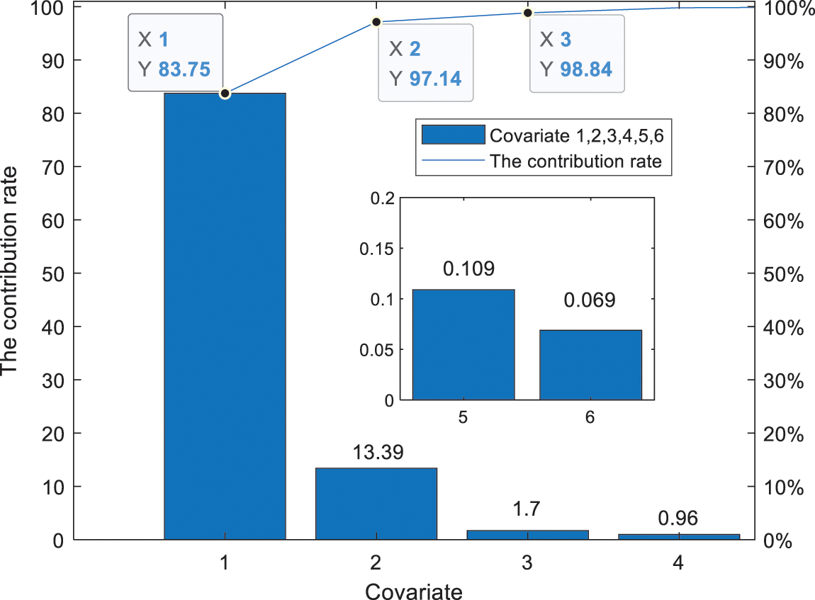
Figure 4: Screening results of the covariate
Fig. 4 shows that the contribution rate of the first three kernel principal components is 98.84%, and they are chosen as the covariates. However, the contribution rate of the kernel principal components after 6 dimensions is too low, so it is no longer shown in Fig. 4. The histogram amplitude corresponds to the left ordinate and is represented as the contribution value of the first kernel principal component to the sixth kernel principal component: 83.75, 13.39, 1.7, 0.96, 0.109, and 0.069.
In this experiment, the hyperparameters of the BWO algorithm are set as follows. “Population size = 50” and “maximum number of generations = 100.” Based on the chosen covariates, the model parameter estimation results are demonstrated in Table 2.

Table 2 shows that the log-likelihood value of the MLE after BWO optimization is −14.956, which is higher than that of the traditional MLE, indicating that the parameter estimation accuracy after BWO optimization is higher. The estimated parameters are introduced into the WPHM model. The cumulative failure rate and reliability results of the rolling bearing are illustrated in Figs. 5 and 6, respectively.
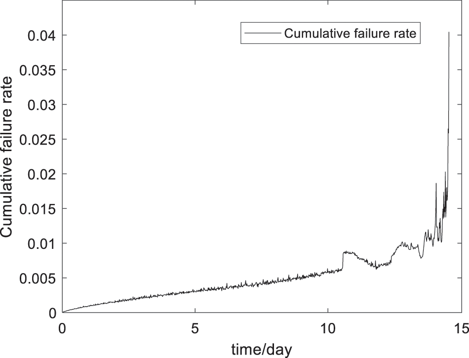
Figure 5: Cumulative failure rate results of the rolling bearing
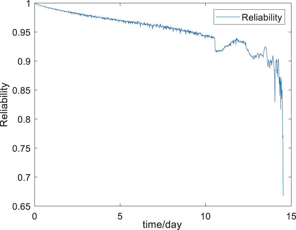
Figure 6: Reliability curves
Fig. 5 shows that the cumulative failure rate of the rolling bearing is proportional to the operating time and that the faults accumulate over the life of the rolling bearing until it fails.
Fig. 6 shows that from the beginning to approximately 10.5 days of operation, the rolling bearing reliability decreases smoothly with a small fluctuation such that the rolling bearing is in the initial normal operation stage, and there are no faults in the rolling bearing. After 10.5 days, the incipient fault occurs, and the failure rate and reliability fluctuate significantly. This is because the faults in the rolling bearing are random, and the reliability of the rolling bearing decreases at this stage. In the recovery stage, which is inevitable for the degeneration of the rolling bearing (at approximately 12.5 days), cracks and scratches in the inner and outer rings of the rolling bearing are smoothed. The operating state of the rolling bearing tends to be stable, and its reliability increases in a short time. Furthermore, owing to the accumulation of faults and fatigue, the reliability of the rolling bearing decreased significantly, and the rolling bearing finally failed. Consequently, the reliability curve fully reflects the entire life cycle process of the rolling bearing operation, which can be the basis for assessing the operating state of the rolling bearing.
5.2 Reliability Prediction Results and Analysis
In this section of the experiment, the degradation data of bearing 1 in experiment 2 where the outer ring failure occurs are selected as the test data, and the data of bearings 3 and 4 in experiment 1 and the data of bearing 3 in experiment 3 are selected as the training data. Then, the reliability curve depicted in Fig. 6 is chosen as the label for reliability prediction so that the reliability prediction of the rolling bearing is implemented. Moreover, the BPNN and support vector machine (SVM) network are utilized for a comparison experiment to show the accuracy of the LSTM network for long-time series prediction. Root mean square error (RMSE), mean absolute error (MAE), and R-Square in the regression evaluation indexes are used to evaluate the experimental results. These indexes are chosen because the existence of large errors in the predicted value increases the value of the RMSE. Absolute values are taken for the error values in the MAE because the positive and negative errors cannot cancel each other out, and the mean absolute error can therefore better reflect the actual prediction error. R-square is used to represent the quality of data fitting; the closer the value is to 1, the better the fitting effect.
In this experiment, the hyperparameters of the LSTM model are set as follows: “Number of neurons in the first layer = 64,” “Number of second layer neurons = 64,” “Learning rate = 0.001,” “Iterations = 100,” and “Batch size = 64.” The hyperparameters of the BPNN model are set as follows: “Learning rate = 0.01,” “Iterations = 1000,” and “Batch size = 500.” The hyperparameters of the SVM model are set as follows: “C = 1.0,” “Kernel = ‘rbf’,” and “gamma = 32.” Based on these hyperparameters, the reliability prediction results are shown in Fig. 7.
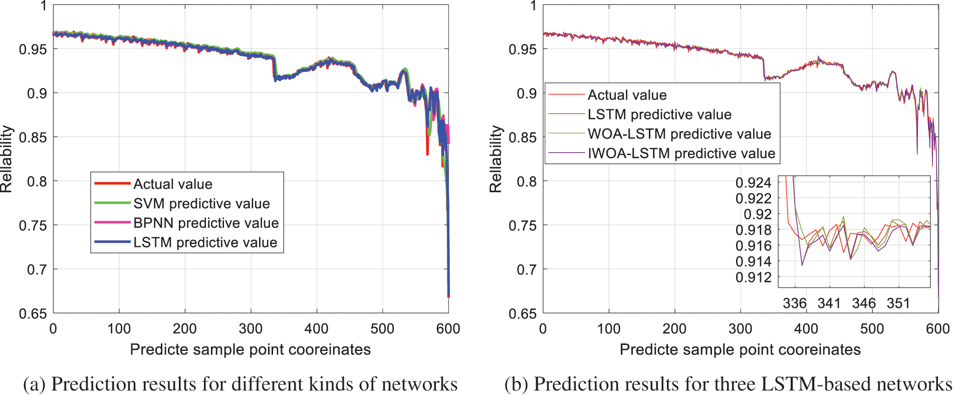
Figure 7: Reliability prediction results
The obtained regression evaluation indexes of the prediction are shown in Table 3.

Fig. 7 shows that the LSTM network better uses time sequence information and performs better prediction compared with the SVM network and BPNN. In particular, at the last stage of the prediction, the prediction and real values are highly fitted, which better reflects the degeneration degrees of reliability. Furthermore, IWOA implements better reliability prediction compared with the WOA-LSTM and LSTM networks. Table 3 illustrates the above discussion. All the regression evaluation indexes obtained by the LSTM network are better than those of the SVM network and BPNN, which shows that the LSTM network better uses time sequence information. Moreover, all the regression evaluation indexes obtained by the IWOA-LSTM network are better than those of the WOA-LSTM and LSTM networks. By calculation, compared with the WOA-LSTM network, the RMSE and MAE of the reliability prediction of the IWOA-LSTM network decreased by 12.5% and 23.5%, respectively; compared with the LSTM network, the RMSE and MAE decreased by 27.6% and 44.9%, respectively. Moreover, compared with the WOA-LSTM and LSTM networks, the R-squares of the reliability prediction of the IWOA-LSTM network increased by 1.2% and 2.2%, respectively. These results fully verify that the proposed IWOA further improves the prediction accuracy of the LSTM network.
5.3 RUL Prediction Results and Analysis
To exclude features with a high degree of similarity in the feature dataset, correlation indexes, such as correlation, robustness, and monotonicity, are used to evaluate the degree of correlation between degeneration features and time. Define
where W denotes the linear superposition of each weighted index;
Set
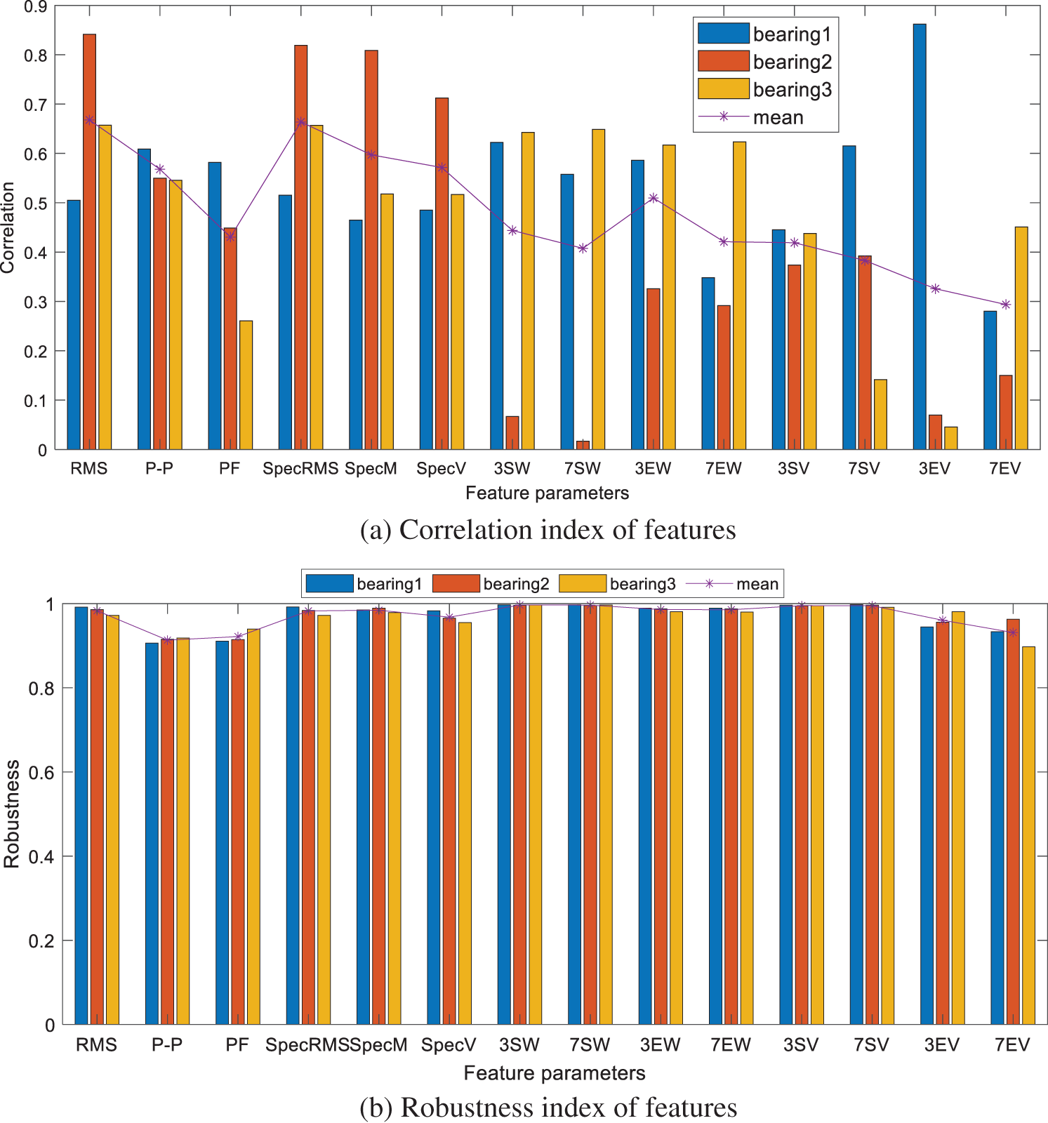
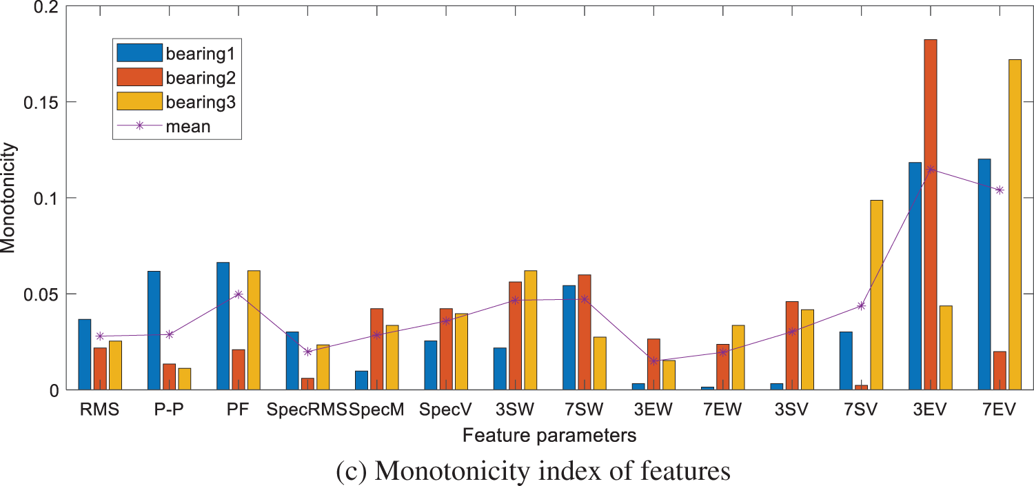
Figure 8: Feature parameter indicators
Furthermore, to guarantee the effectiveness of the screened feature parameters, the screening threshold is chosen as 0.435, and the screening process is shown in Fig. 9.
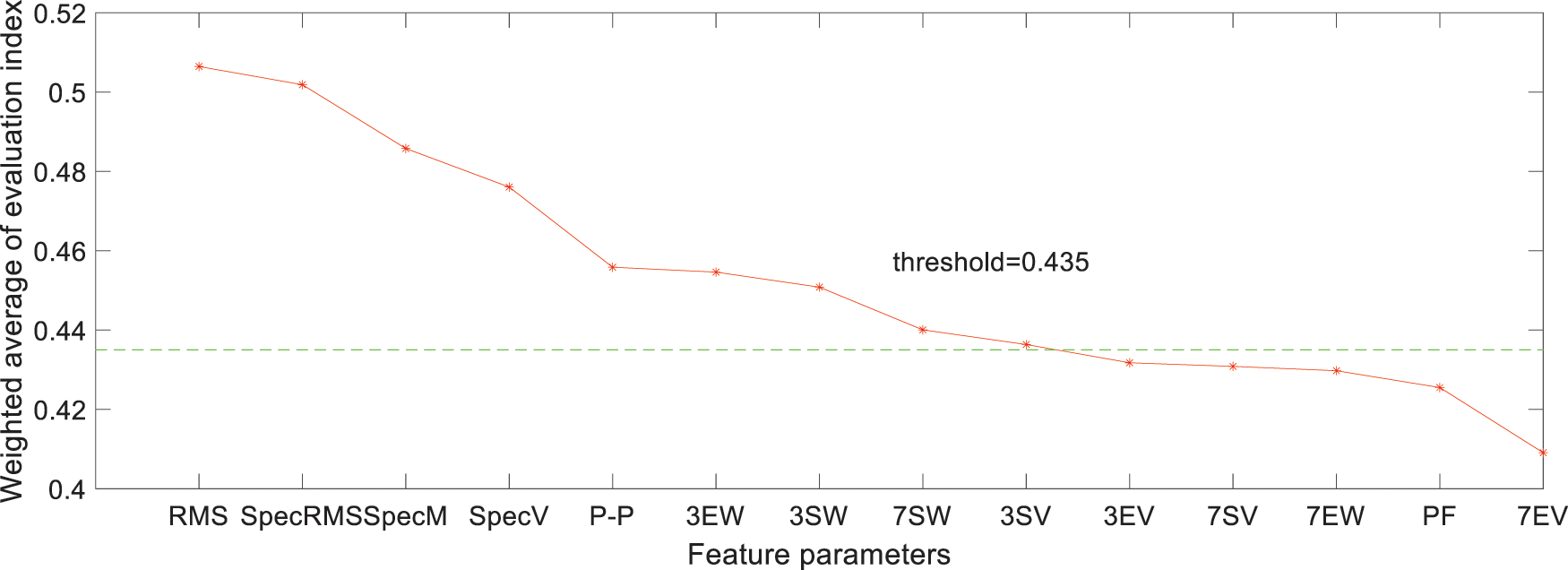
Figure 9: Ranking results of feature parameters
Based on Fig. 9, 9 effective features are screened from the feature dataset, including 14 feature parameters obtained in Section 2, and the screened results are shown in Fig. 10. The analysis shows that the screened feature parameters reflect the degeneration process of the life cycle of the rolling bearing and verifies the effectiveness of the evaluation indexes of the feature parameters simultaneously.
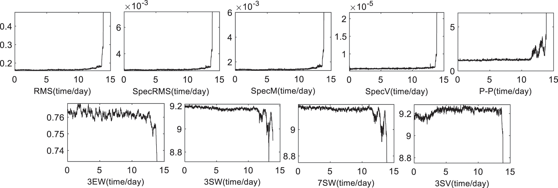
Figure 10: The degradation feature parameters
Based on Fig. 10, 9 screened features are combined with the reliability curve as the input of the IWOA-LSTM network. Using the proposed IWOA-LSTM network for the RUL prediction, in this experiment, the hyperparameters of the IWOA algorithm are set as follows: “Population size = 100” and “Maximum number of generations = 10”. The optimization results for the hyperparameters are depicted in Fig. 11.
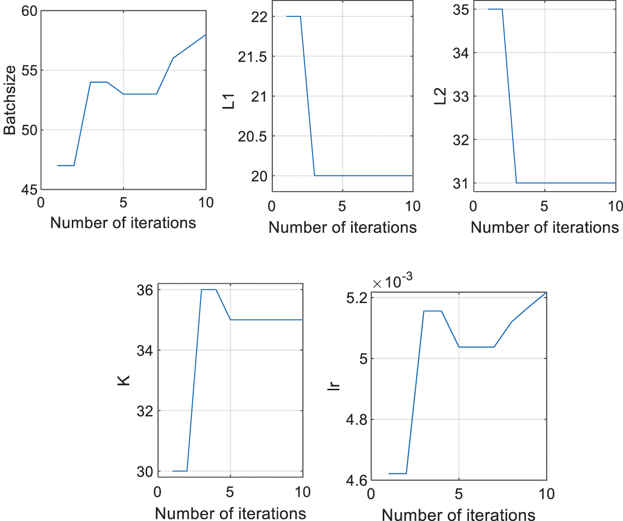
Figure 11: Changes in hyperparameters in the IWOA
Fig. 11 shows the parameters of the LSTM network as batch size; the number of neurons in the first layer, the number of neurons in the second layer, the number of iterations, and the learning rate are all optimized from the original random values to suitable values using the proposed IWOA.
In this study, to implement a comparison experiment, the hyperparameters of the LSTM networks are optimized using WOA and IWOA. The optimized hyperparameters of the LSTM model are set as shown in Table 4. The RUL prediction results of the IWOA-LSTM network are compared with those of the WOA-LSTM and LSTM networks are shown in Fig. 12.

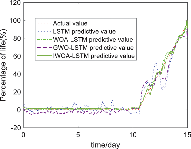
Figure 12: RUL prediction results
Fig. 12 shows that the IWOA-LSTM network implements the best RUL prediction, and the prediction results of the IWOA-LSTM network fit the real RUL curve. This is because the proposed adaptive threshold and nonlinear adaptive weights improve the ability of the WOA to jump out of local optimization. In this way, the IWOA implements better-optimizing ability. The WOA-LSTM and GWO-LSTM networks implement a better RUL prediction compared with the traditional LSTM network, as the WOA and GWO avoid the randomness of the manual selection for key parameters of the LSTM network.
To further illustrate the effectiveness of the proposed method, the obtained regression evaluation indexes, such as RMSE, MAE, and R-square, are listed in Table 5.
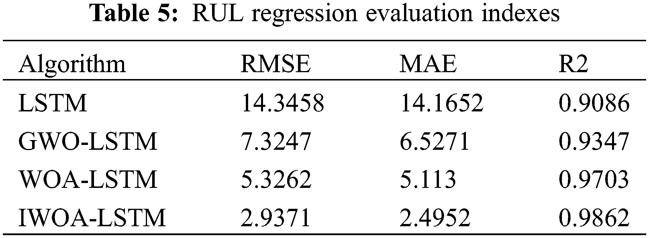
Table 5 shows that the RMSE and MAE of the IWOA-LSTM network are less than 3, which is smaller than those of the other three LSTM-based networks. Moreover, the R-square of the IWOA-LSTM network is greater than 0.986, which is closer to 1 compared with that of the other three LSTM-based networks. By calculation, compared with the WOA-LSTM, GWO-LSTM, and LSTM networks, the RMSEs of the RUL prediction decreased by 18.8%, 59.9%, and 79.5%, respectively; the MAEs decreased by 51.2%, 61.77%, and 82.4%; and R-squares increased by 1.6%, 5.2%, and 7.9%, respectively. The results shown in Fig. 12 and Table 5 further verify the effectiveness of the proposed method.
Based on the above discussion, using the reliability assessment results based on the KPCA and the WPHM, the reliability prediction and RUL prediction results obtained by the IWOA-LSTM network are better than those of the WOA-LSTM network. These results verify that the proposed adaptive threshold and the nonlinear adaptive nonlinear weights improve the capability of the WOA to jump out of the local optimization; therefore, the prediction accuracy of the LSTM network is further improved. The experimental results comprehensively illustrate the effectiveness of the proposed method for reliability prediction and RUL prediction.
In this study, a reliability prediction and RUL prediction method for a rolling bearing based on an optimized neural network was proposed. Based on signal processing methods, the features of the time, frequency, and time–frequency domains were extracted from the original vibration signals, and a feature dataset was established. Using the KPCA, the feature dataset dimension reduction was implemented. To improve the accuracy of the reliability assessment, the WPHM was constructed using the optimal parameters obtained using the BWO-MLE. To characterize the rolling bearing degradation process, the main evaluation indexes for degradation features during the entire life cycle, namely, correlation, monotonicity, and robustness, were used to evaluate the suitability of the feature parameters. Using the adaptive threshold and nonlinear adaptive parameters, an IWOA was proposed to optimize the global searching ability of the LSTM networks. The IWOA avoided the inaccurate manual selection of the hyperparameters, and the accuracy of the reliability prediction and RUL prediction was improved. Experimental results showed that compared with previous studies, the proposed prediction model implemented a better reliability prediction and RUL prediction for the rolling bearing.
Acknowledgement: None.
Funding Statement: This paper was supported by the Department of Education of Liaoning Province under Grant JDL2020020 and the Transportation Science and Technology Project of Liaoning Province under Grant 202243.
Author Contributions: The authors confirm contribution to the paper as follows: study conception and design: R Wang, T Liang; data collection: Y Wang, J Yang; analysis and interpretation of results: R Wang, X Zhang; draft manuscript preparation: R Wang, Y Wang. All authors reviewed the results and approved the final version of the manuscript.
Availability of Data and Materials: The data that support the findings of this study are available from the corresponding author upon reasonable request.
Conflicts of Interest: The authors declare that they have no conflicts of interest to report regarding the present study.
References
1. He, M., He, D. (2018). Simultaneous bearing fault diagnosis and severity detection using a LAMSTAR network-based approach. IET Science, Measurement and Technology, 12(7), 893–901. https://doi.org/10.1049/iet-smt.2017.0528 [Google Scholar] [CrossRef]
2. Mao, W., Tian, S., Fan, J., Liang, X., Safian, A. (2022). Online detection of bearing incipient fault with semi-supervised architecture and deep feature representation. Journal of Manufacturing Systems, 55, 179–198. https://doi.org/10.1016/j.jmsy.2020.03.005 [Google Scholar] [CrossRef]
3. Wu, J., Wu, C., Cao, S., Or, S. W., Deng, C. et al. (2018). Degradation data-driven time-to-failure prognostics approach for rolling element bearings in electrical machines. IEEE Transactions on Industrial Electronics, 66(1), 529–539. https://doi.org/10.1109/TIE.2018.2811366 [Google Scholar] [CrossRef]
4. Cao, X., Li, P., Ming, S. (2021). Remaining useful life prediction-based maintenance decision model for stochastic deterioration equipment under data-drive. Sustainability, 13(15), 8548. https://doi.org/10.3390/su13158548 [Google Scholar] [CrossRef]
5. Guo, J., Li, Z., Li, M. (2019). A review on prognostics methods for engineering systems. IEEE Transactions on Reliability, 69(3), 1110–1129. https://doi.org/10.1109/TR.2019.2957965 [Google Scholar] [CrossRef]
6. Helmi, H., Forouzantabar, A. (2019). Rolling bearing fault detection of electric motor using time domain and frequency domain features extraction and ANFIS. IET Electric Power Applications, 13(5), 662–669. https://doi.org/10.1049/iet-epa.2018.5274 [Google Scholar] [CrossRef]
7. Chen, Q., Wen, D., Li, X., Chen, D., Lv, H. et al. (2019). Empirical mode decomposition based long short-term memory neural network forecasting model for the short-term metro passenger flow. PLoS One, 14(9), e0222365. https://doi.org/10.1371/journal.pone.0231199 [Google Scholar] [CrossRef]
8. Meng, D., Wang, H., Yang, S., Lv, Z., Hu, Z. et al. (2022). Fault analysis of wind power rolling bearing based on EMD feature extraction. Computer Modeling in Engineering & Sciences, 130(1), 543–558. https://doi.org/10.32604/cmes.2022.018123 [Google Scholar] [CrossRef]
9. Shi, H., Guo, J., Yuan, Z., Liu, Z., Hou, M. et al. (2020). Incipient fault detection of rolling element bearings based on deep EMD-PCA algorithm. Shock and Vibration, 2020, 1–17. https://doi.org/10.1155/2020/8871433 [Google Scholar] [CrossRef]
10. Zhang, Y., Chen, B., Pan, G., Zhao, Y. (2019). A novel hybrid model based on VMD-WT and PCA-BP-RBF neural network for short-term wind speed forecasting. Energy Conversion and Management, 195, 180–197. https://doi.org/10.1016/j.enconman.2019.05.005 [Google Scholar] [CrossRef]
11. Niu, H., Xu, K., Wang, W. (2020). A hybrid stock price index forecasting model based on variational mode decomposition and LSTM network. Applied Intelligence, 50(12), 4296–4309. https://doi.org/10.1007/s10489-020-01814-0 [Google Scholar] [CrossRef]
12. Cheng, Y., Wang, J., Wu, J., Zhu, H., Wang, Y. (2023). Abnormal symptom-triggered remaining useful life prediction for rolling element bearings. Journal of Vibration and Control, 29(9–10), 2102–2115. https://doi.org/10.1177/10775463221074797 [Google Scholar] [CrossRef]
13. Santhosh, T. V., Gopika, V., Ghosh, A. K., Fernandes, B. G. (2018). An approach for reliability prediction of instrumentation & control cables by artificial neural networks and Weibull theory for probabilistic safety assessment of NPPs. Reliability Engineering & System Safety, 170, 31–44. https://doi.org/10.1016/j.ress.2017.10.010 [Google Scholar] [CrossRef]
14. Wang, Y., Chen, Z., Zhang, Y., Li, X., Li, Z. (2020). Remaining useful life prediction of rolling bearings based on the three-parameter Weibull distribution proportional hazards model. Insight-Non-Destructive Testing and Condition Monitoring, 62(12), 710–718. https://doi.org/10.1784/insi.2020.62.12.710 [Google Scholar] [CrossRef]
15. Li, Y. F., Liu, Y., Huang, T., Huang, H. Z., Mi, J. (2020). Reliability assessment for systems suffering common cause failure based on Bayesian networks and proportional hazards model. Quality and Reliability Engineering International, 36(7), 2509–2520. https://doi.org/10.1002/qre.2713 [Google Scholar] [CrossRef]
16. Jokiel-Rokita, A., Pia¸tek, S. (2022). Estimation of parameters and quantiles of the Weibull distribution. Statistical Papers, 1–18. https://doi.org/10.1007/s00362-022-01379-9 [Google Scholar] [CrossRef]
17. Algamal, Z. Y., Basheer, G. (2021). Reliability estimation of three parameters Weibull distribution based on particle swarm optimization. Pakistan Journal of Statistics and Operation Research, 17(1), 35–42. https://doi.org/10.18187/pjsor.v17i1.2354 [Google Scholar] [CrossRef]
18. Zhu, L., Chen, D., Feng, P. (2021). Equipment operational reliability evaluation method based on RVM and PCA-fused features. Mathematical Problems in Engineering, 2021(9), 1–9. https://doi.org/10.1155/2021/6687248 [Google Scholar] [CrossRef]
19. Gao, S., Yu, Y., Zhang, Y. (2022). Reliability assessment and prediction of rolling bearings based on hybrid noise reduction and BOA-MKRVM. Engineering Applications of Artificial Intelligence, 116, 105391. https://doi.org/10.1016/j.engappai.2022.105391 [Google Scholar] [CrossRef]
20. Liu, X., Liu, Z., Liang, Z., Zhu, S. P., Correia, J. A. et al. (2019). PSO-BP neural network-based strain prediction of wind turbine blades. Materials, 12(12), 1889. https://doi.org/10.3390/ma12121889 [Google Scholar] [PubMed] [CrossRef]
21. Shang, S., He, K. N., Wang, Z. B., Yang, T., Liu, M. et al. (2020). Sea clutter suppression method of HFSWR based on RBF neural network model optimized by improved GWO algorithm. Computational Intelligence and Neuroscience, 2020. https://doi.org/10.1155/2020/8842390 [Google Scholar] [PubMed] [CrossRef]
22. Hu, Y. L., Chen, L. (2018). A nonlinear hybrid wind speed forecasting model using LSTM network, hysteretic ELM and differential evolution algorithm. Energy Conversion and Management, 173, 123–142. https://doi.org/10.1016/j.enconman.2018.07.070 [Google Scholar] [CrossRef]
23. Mahmoodzadeh, A., Nejati, H. R., Mohammadi, M., Ibrahim, H. H., Rashidi, S. et al. (2022). Forecasting tunnel boring machine penetration rate using LSTM deep neural network optimized by grey wolf optimization algorithm. Expert Systems with Applications, 209, 118303. https://doi.org/10.1016/j.eswa.2022.118303 [Google Scholar] [CrossRef]
24. Wang, S., Li, P., Ji, H., Zhan, Y., Li, H. (2021). Prediction of air particulate matter in Beijing, China, based on the improved particle swarm optimization algorithm and long short-term memory neural network. Journal of Intelligent & Fuzzy Systems, 41(1), 1869–1885. https://doi.org/10.3233/JIFS-210603 [Google Scholar] [CrossRef]
25. Wang, W., Tang, Q. (2022). Combined model of air quality index forecasting based on the combination of complementary empirical mode decomposition and sequence reconstruction. Environmental Pollution, 120628. https://doi.org/10.1016/j.envpol.2022.120628 [Google Scholar] [PubMed] [CrossRef]
26. Qiu, H., Lee, J., Lin, J., Yu, G. (2006). Wavelet filter-based weak signature detection method and its application on rolling element bearing prognostics. Journal of Sound and Vibration, 289(4–5), 1066–1090. https://doi.org/10.1016/j.jsv.2005.03.007 [Google Scholar] [CrossRef]
27. Zhong, C., Li, G., Meng, Z. (2022). Beluga whale optimization: A novel nature-inspired metaheuristic algorithm. Knowledge-Based Systems, 251, 109215. https://doi.org/10.1016/j.knosys.2022.109215 [Google Scholar] [CrossRef]
Cite This Article
 Copyright © 2023 The Author(s). Published by Tech Science Press.
This work is licensed under a Creative Commons Attribution 4.0 International License , which permits unrestricted use, distribution, and reproduction in any medium, provided the original work is properly cited.


 Submit a Paper
 Propose a Special lssue
 View Full Text
 Download PDF
 Downloads
 Citation Tools