Outlier Detection and Forecasting for Bridge Health Monitoring Based on Time Series Intervention Analysis

1  Introduction

In recent years, bridge health monitoring (BHM) system has become an inseparable part in not only super-major and major bridges but also small and medium-sized bridges. Vast amounts of monitoring data, which contain a variety of characteristic information of the structure under the operation phase, flow into BHM system every day. How to make effective use of the monitoring data for in-depth mining is of vital importance for bridge early warning and assessment [1,2]. However, in the process of feature extraction, the complexity of the identification problem has far exceeded the traditional data processing capability and understanding mode in the domain of structural engineering, due to its nonlinearity, incompleteness, and noise interference, which brings huge challenges to bridge monitoring. The phenomenon of “Rich data but poor knowledge” is widely observed in the existing BHM systems [3,4]. Big data theory, which has rapidly risen and improved of late years, provides a possible breakthrough for the processing of massive monitoring data [5–8]. Sun et al. [9,10] investigated the research orientation and application status of big data in bridge health monitoring, established the big data analysis framework and pointed out that current research on big data in the field of bridge health monitoring is still at the initial stage, but it has got a lot of potential.

Time series techniques, originally developed for analyzing long sequences of regularly sampled data, are inherently suitable for BHM. Time series forecasting methods can be broadly classified into two main categories, namely statistical methods and deep learning methods. The performance of each method depends on multiple factors such as trend, seasonality and noise in the data, as well as external conditions and internal damages [11,12].

Deep learning (DL) techniques, which can automatically learn the temporal dependencies present in time series and effectively reduce the complexity of the forecasting pipeline, have proved to be an effective solution in time series forecasting, and have gained considerable prominence [13,14]. Oh et al. [15] proposed a CNN-based architecture to predict strain levels of tall buildings under wind loadings. The training dataset containing displacements and wind speeds was collected from a wind tunnel test of a model of a steel structure. Peng et al. [16] adopted piecewise linear least squares (PLLS) method, fully connected neural network (FCNN) method, and long short-term memory neural network (LSTMNN) method to predict the structural dynamic response of a six-story steel frame under periodic, impact, and seismic loads. Results showed that the LSTMNN method performed better than the other two methods. In addition, the PLLS method was sensitive to noise, while the FCNN and LSTMNN methods based on deep learning were of highly robust and anti-noise performance. Zheng et al. [17] established an LSTM neural network for modeling multiple temperature-displacement correlations. The results revealed that compared with the BP neural network model, the proposed LSTM neural network model could dramatically reduce the reproduction error and prediction error of the thermal displacement.

Time series analysis is one of the statistical procedures applied to simulate the degradation mechanism of bridge structures and make predictions by establishing various time series data mining models and algorithms that can reflect the variation of variables in the time domain [18–20]. van Le et al. [21] used ARIMA model for the analysis of the GPS time series data acquired in a cable-stayed bridge in Vietnam, and data were used to predict the static responses and global deformation. Conclusions were drawn that the AR-MA coefficients plots could be used as the base distributions for the statistical structural condition assessment. Zhu et al. [22] proposed a combination forecast model based on CEEMDAN-NAR-ARIMA, and used it to predict the SHM strain data of a cable-stayed bridge in Shanghai. Results showed that the proposed method was more accurate than classical time series theory. Ahmadivala et al. [23] applied seasonal ARIMA on the mean values of strain monitoring data on Chillon viaducts for every 12 h, so as to explore more details of the loading scenario regarding the seasonal effects of traffic loading. Xin et al. [24] used the Kalman filter to reduce the noise of the bridge’s raw deformation data and developed ARIMA-GARCH model to analyze and predict the structure’s deformation. Shi et al. [25] decomposed the observed SHM time series into three components, namely, level, seasonal and residual, and purged the influence of seasonality, in order to obtain a more agreeable series that could reflect the characteristics of structural damage. Jiang et al. [26] adopted ARIMA model integrated with singular spectrum analysis (SSA) for a more precise prediction of stress monitoring data of Sutong bridge.

It can be seen that an appropriate time series model or combination model does better explain the characteristics of nonlinearity, non-stationarity, high dimensionality and heteroscedasticity of monitoring data. However, these models were built on the assumption that the monitoring data were accurate and reliable [27,28]. In a long-term continuous monitoring system, the regular data collection is inevitably disturbed by accidental extreme loads, external forces on the sensors themselves, abnormal current or voltage, power failure, sensor damage, etc. These external interruptive events, referred to as interventions, may create spurious observations that are inconsistent with the rest of the series and interfere with the identification of the time series model [29]. Therefore, identification and characterization of outlier interventions are important from the point of view of BHM management as these events could probably reduce the precision of the forecast results of structural behavior.

However, from the existing literature, most of the studies focus on the selection of the most convenient type of time series model and its parameter recognition and estimation [30,31]. Research that discusses the intervention effect of outliers on fitted precision of the models and on assessment of structural behavior is rarely seen. Therefore, in this study, the possible abnormal conditions in bridge monitoring data are investigated from the perspective of intervention analysis. First, a brief description of the SARIMA model with outliers is outlined. The methodology of outlier detection and amendment then follows, and the identification and prediction of time series model containing outliers are discussed. The proposed procedure is then used to identify the outliers from strain data recorded by a BHM system and to predict the structural future condition.

The main purpose of outlier correction is to optimize the data in such a way that the normality hypothesis of the SARIMA model can be better accepted. Moreover, by containing outlier intervention effect in the SARIMA model, the residual variance of the model is reduced, the fitting precision of the model is significantly improved, and the accuracy and reliability of the forecast are strengthened.

2  Nonstationary SARIMA Models

Under the influence of external loads and structural performance degradation, the monitoring responses of bridge structures exhibit randomness in a short period of time. However, from a longer time perspective, the monitoring time sequences will present certain regularity, such as long-term trend, periodicity, random fluctuation, and mutation. As can be seen from the sequence diagram of observed data, there exists significant non-stationarity in some of the monitoring series, while others have conspicuous seasonal characteristics due to the effect of seasonal temperature difference. Therefore, the seasonal ARIMA model is introduced to fit and analyze the nonstationary bridge monitoring data [32].

Assume {Yt} is a time series observed from a certain sensor on BHM system, and {ε1, ε2, …, εt} is a zero-mean multivariate Gaussian white noise series. If a stationary series can be obtained by taking a dth-order nonseasonal difference ∇d and a Dth-order seasonal difference with period s ∇sD , then the general SARIMA model can be represented analytically as

{Φ(B)Ψ(Bs)∇d∇sDyt=Θ(B)H(Bs)εtE(εt)=0,Var(εt)=σε2,cov(εh,εt)=0,h≠tcov(yh,εt)=0,∀h<t (1)

The model in Eq. (1) is normally denoted as ARIMA (p, d, q) × (P, D, Q)s, where Φ(B)=1−ϕ1B−⋯ϕpBp is the nonseasonal autoregressive (AR) operator of order p, Θ(B)=1−θ1B−⋯θqBq is the nonseasonal moving average (MA) operator of order q, and polynomials Ψ(Bs)=1−ψ1Bs−ψ2B2s−⋯ψpBPs and H(Bs)=1−η1Bs−η2B2s−⋯ηqBQs respectively describe the seasonal AR and MA operators of orders P and Q with seasonal period s; ϕi, θi, ψi, ηi (i = 1, …, n) are the coefficients of Φ(B), Θ(B), Ψ(Bs) and H(Bs), respectively; and B is the backward shift operator such that Bkyt = yt−k. E(εt) and Var(εt) are the mean function and the variance function of the Gaussian white noise series {εt}, respectively, and cov(εh, εt) is the correlation function between εh and εt.

In particular, when there is an additive relationship between the seasonal effect and other effects in the series, the seasonal information can be fully extracted by taking a first difference with periodic step length. At this point, the model can be simplified into Eq. (2), which is denoted as ARIMA (p, d, q) × (0, D, 0)s.

Nt=Θ(B)Φ(B)∇d∇sDεt (2)

Generally speaking, the measured responses of the structure can be considered as the linear superposition of various load effects when the structure is in the normal operation state. Therefore, for the observed time series with seasonal effect, the seasonal additive model shown in Eq. (2) is adequate to describe the actual state of the structure.

Fig. 1 displays the procedure for the establishment of SARIMA models.

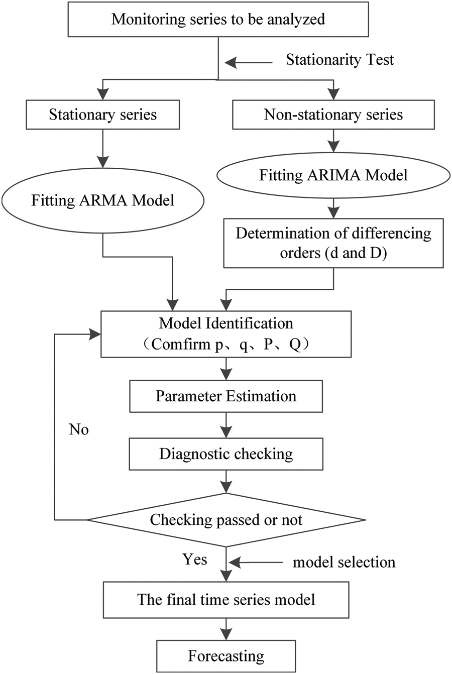
Figure 1: Flow chart of SARIMA modeling process

3  Time Series Analysis with Outlier Intervention

3.1 SARIMA Model Containing Outlier Effects

To consider the influence of different types of intervention outliers, the indicator function is introduced. Thus, the general model of time series {Yt}, which contains outlier information, can be written as the combination of various indicator functions shown in Eq. (3) [33].

Yt=Gt+Nt=c+∑i=1kωi(B)Bbiδi(B)Iti+Nt (3)

where Gt represents the influence of interventions expressed in the form of indicator function using deterministic intervention variables Iti; k is the total number of outliers; B is the delay operator; b denotes the time delay for the intervention effects, and for bridge structure, b = 0, on account of the instantaneous response to the external action; ω(B) reflects the intensity of intervention and δ(B) measures the behavior of the permanent effect of the intervention. Additionally, the time series free of intervention is called the noise series or the undisturbed series and is denoted by Nt. Nt can be various kinds of stationary or non-stationary series. For a nonstationary process, the model in Eq. (3) normally does not contain a constant term c.

When there are outliers detected in monitoring data, the abnormal behavior can be explained by intervention analysis techniques if the timing and causes of interruptions are knowable. However, the timing of interventions is usually unknown. So, it is necessary to detect and estimate the possible effects. Here, two common outlier models, innovational outlier (IO) and additive outlier (AO), are introduced [34].

Let Nt be an undisturbed process free of interventions and follow an additive SARIMA process ARIMA (p, d, q) × (0, D, 0)s defined in Eq. (2).

(1)    If the error εt of Nt at time T is disturbed and turned into εt′=εt+ωPt(T) , the post-disturbed series can be described using an IO model

Yt=Θ(B)Φ(B)∇d∇sD(εt+ωPt(T))=Nt+ω(Θ(B)Φ(B)∇d∇sD)Pt(T)(4)

where Pt(T) is a pulse function taking place at T time period which can be written as

Pt(T)={0,t≠T1,t=T(5)

(2)    If Nt is subject to additive disturbance at time T, the AO model is introduced as

Yt=Nt+ωPt(T) (6)

Hence, an AO affects only the Tth observation by the intensity ω when the interruption takes place. While an IO describes the systematic dynamic behavior by Θ(B)/Φ(B)∇d∇sD , and affects all observations YT, YT+1,… beyond time T.

(3)    If a time series is influenced by k outliers of different types at different time periods T1, T2, … Tk, a more general model containing various types of outliers is presented as follows:

Yt=Nt+∑i=1kωiLi(B)Pt(Ti)(7)

where, for SARIMA model

Li(B)={Θ(B)Φ(B)∇d∇sD,IO1,AO⋯(8)

3.2 Outlier Mining

When outliers exist, the estimated parameters are biased. In this case, appropriate test statistics are constructed from the residuals, which are the discrepancies between the observed and the estimated values, for the detection and correction of outliers. Outlier mining based on time series analysis is to identify the time, size and types of outliers, estimate their impacts, and modify the original time series model affected by outliers so as to improve the accuracy of the model.

Let {Yt} be the original observed monitoring series, which can be fitted by an additive SARIMA model as Eq. (2). The hypothesis test is performed as follows:

H0: yT is neither an IO nor an AO

H1: yT is an IO

H2: yT is an AO

The process of outliers detection is mainly discussed in the following two cases [35].

(1)    Only one type of outlier is included, and the timing of the outlier occurrence is known.

The residual series of IO and AO models can be written respectively as

et={ωIPt(T)+εt,IOωAπ(B)Pt(T)+εt,AO (9)

where π(B)=Φ(B)∇d∇sDΘ(B)=1−π1B−⋯πnB2−⋯

According to the least-squares principle, when t = T, the least-square estimator of the disturbance ωI or ωA (shown in Eq. (10)) is the residual at time T (IO) or the linear combination of the residuals (AO).

{IO:ω^I,T=eTAO:ω^A,T=−ρ2∑t=1nπt−Tet (10)

where ρ2=(1+π12+π22+⋯πn−T2)−1 . Thus, the variance of the estimator is

{Var(ω^I,T)=Var(eT)=Var(ωIPt(T)+εt)=σa2Var(ω^A,T)=ρ2σa2 (11)

The test statistics for IO and AO at time T are

{λI,T=ω^I,TσaλA,T=ω^A,Tρσa (12)

Under the null hypothesis H0, ωI = 0 and ωA = 0, and both λI,T and λA,T are distributed as N(0, 1). Let the significance level be α = 0.05, then the necessary condition for accepting hypothesis H1 or H2 is respectively λI,T > 1.96 or λA,T  > 1.96.

(2)    The timing and type of the outliers are unknown.

Case (1) is applicable to situations where the timing and type of the outliers are known. However, more often in practice, the type, timing and number of outliers are unknown and have to be estimated. An iterative detection procedure is proposed to handle the situation when an unknown number of AO or IO may exist [36,37]. Specifically, the following four steps are included:

Step 1. Model the original monitoring series {Nt} with SARIMA supposing that there are no outliers. The residual series can be derived as

εt=π(B)Nt=Φ(B)∇d∇sDΘ(B)Nt (13)

The initial estimate of the standard deviation of the residuals is

σ^ε=1n∑t=1nε^t2 (14)

Step 2. Perform statistical tests of outliers using the initial residuals estimated at t = 1, 2, 3, … , n. The test statistics for IO and AO refer to Eq. (12). Thus, λI,T and λA,T for each time period can be calculated. Define

λ^t=maxt⁡[max(|λI,t|,|λA,t|)],t=1,2,…,n (15)

where λ^t denotes the maximum outlier at different times.

Bonferroni correction is used to control the overall error rate of multiple tests. Based on 0.05 significance level, if the p-value of λ^t at time T is greater than the upper percentile of the standard normal distribution, or λ^t>C , where C is a predetermined positive constant usually taken to be some value between 3 and 4, then there is an outlier at time T with its type determined by λI,T or λA,T.

It should be noted that the maximum likelihood estimation of σε is on the high side in the presence of outliers. Especially when the sample size is small, such deviation may become very great, resulting in a reduction of λ^t . To eliminate the influence of outliers on σε, the robust estimation is adopted to replace the maximum likelihood estimation. In the latter example, the absolute mean of the residual is multiplied by 2/π to get a more robust estimate.

According to different types of outliers, the effect of IO/AO at time T can be removed by modifying the data using Eq. (16) as

Y~t={Yt−ωI,Tπ(B)Pt(T),IOYt−ωA,TPt(T),AO (16)

where π(B)=Φ(B)∇d∇sDΘ(B)=1−π1B−⋯πnB2−⋯ , and the new residual sequence is defined as

ε~t={et−ω^I,T,IOet−ωA,Tπ(B)Pt(T),AO (17)

The new estimate of the standard deviation of the residuals σ~ε can be recalculated from the modified residuals.

Step 3. Re-compute λI,T or λA,T at every time point based on the modified ε~t and σ~ε , and repeat Step 2 to continue detection and modification of outliers until all outliers are identified. In this process, the initial parameter estimates in SARIMA remain unchanged.

Step 4. Suppose that k outliers have been identified at times T1, T2, …, Tk through the first three steps. Treat these times as if they have already been known, then the k outlier parameters ω1, ω2, …, ωk as well as Θ(B) and Φ(B) can be re-estimated. And a new model containing k outliers information can be written as

Yt=Θ(B)Φ(B)∇d∇sDεt+∑j=1kωjLj(B)Pt(Tj) (18)

where Lj(B) is determined by Eq. (8). The new residual series can then be derived from the new fitted model

ε^t=π^(B)[Yt−∑j=1kω^jL^j(B)Pt(Tj)] (19)

and a revised estimate of σ~ε can further be calculated.

Repeat Step 2 to Step 4 until no new outlier is identified.

3.3 Model Forecasting

One of the most important aims of time series analysis is to predict or forecast future development trends of observed data using the fitted models. This is also an important purpose for bridge health monitoring, to figure out the current state of the bridge structure and predict its future long-term development trends through the observed monitoring data.

Consider the general additive seasonal ARIMA (p, d, q) × (0, D, 0)s model shown in Eq. (2). Let Φ∗(B)=Φ(B)(1−B)d(1−Bs)D=1−ϕ~1B−ϕ~2B2−⋯−ϕ~p+d+sDBp+d+sD be the generalized autocorrelation function. And the model can be rewritten in the form of a linear function expressed by the disturbance term

yt=Θ(B)Φ∗(B)εt=Γ(B)εt=(1+γ1B+γ2B2+⋯)εt=εt+γ1εt−1+γ2εt−2+⋯ (20)

Let time t be the forecast origin, l be the lead time for the forecast, and the forecast that will occur l time units into the future be y^t(l) . Then, the mean square error (MSE) of the forecast is

E[yt+l−y^t(l)]2=(1+γ12+⋯+γl−12)σε2+∑j=0∞(γl+j−γj∗)2σε2 (21)

According to the minimum mean square error principle, the MSE shown in Eq. (22) is minimized if and only if γj∗=γl+j . Hence, we have the l-step ahead forecast

y^t(l)=E(yt+l|yt,yt−1,⋯)=γlεt+γl+1εt−1+γl+2εt−2+⋯ (22)

The forecast error is

et(l)=εt+l+γ1εt+l−1+⋯+γl−1εt+1 (23)

with the forecast error variance

Var[et(l)]=Var(yt+l|yt,yt−1,⋯)= (1+γ12+⋯+γl−12)σε2 (24)

It can be seen that the variance of the forecast is only related to step size l, and the forecast error becomes larger and larger as the forecast lead time l increases. Assuming that the value of yt+l obeys the normal distribution under the condition that yt, yt−1, …, are known, the confidence interval of the predicted value yt+l at the confidence level of 1 − α can be obtained as

(y^t(l)−z1−α/2⋅Var[et(l)],y^t(l)+z1−α/2⋅Var[et(l)]) (25)

where z1−α/2 is the standard normal percentile, such that P(–z1−α/2 < Y < z1−α/2) = 1 – α.

4  Application Analysis and Results

4.1 Selection of Monitoring Data Samples

Kunshan Yufeng bridge, located in Kunshan city, Jiangsu Province, is a non-thrusting leaning-type arch bridge with a main span of 110 m (see Fig. 2). In this structural system, the two vertical main arch ribs in the middle and the rigid tie beams (main beams) under the main arch ribs are the major longitudinal load-bearing members, while the inclined arch ribs outward mainly bear part of the dead and live loads and improve the stability of the structure. According to the vulnerability analysis results of the bridge, a total of 43 monitoring points are arranged in 13 sections or positions within the half span of the bridge, aiming at performing a real time monitoring of strain, temperature and support displacement of the critical stressed members. Fig. 3 shows some of the sensors on the bridge and the data collection module.

Figure 2: Kunshan Yufeng bridge

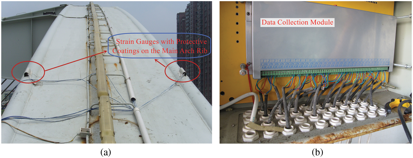
Figure 3: Sensors on the bridge. (a) Strain gauges with protective coatings on the main arch rib; (b) Data collection module

The monitoring data, which are chosen as the modeling basis, are picked from the stress measuring point at the bottom of the vault of the southwest main arch rib of Kunshan Yufeng bridge (Gauge S1-2), with the date ranging from August 23rd, 2011 to February 28th, 2014. These data are presented in the form of weekly-cycle mean value (M value). The weekly cycle here is not strictly measured by the traditional week. We uniformly divide each month into four weeks, namely, 1st∼7th, 8th∼15th, 16th∼23rd and 24th∼30th (31st) (For February, 7th, 14th and 21st are taken as the split nodes). In this way, a year is fixedly divided into 48 weeks, giving a total of 117 sample data. The first 105 monitoring data are used for the model calibration, while the remaining for verification. The weekly-cycle stress M-value of the first 105 data of the sample series is drawn in Fig. 4.

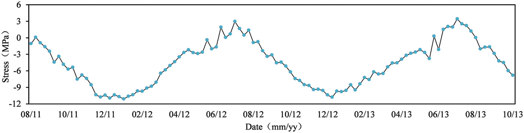
Figure 4: Weekly-cycle M-value of stresses at gauge S1-2

4.2 Establishment of SARIMA Model

The series shown in Fig. 4 implies a clear yearly (48-week) seasonal component, which indicates a typical non-stationary series. Thus, a seasonal ARIMA model is adopted to fit the experimental data. The original data are differenced using operators (1 − B) and (1 − B48) once each. Then, PP test and KPSS test are implemented to the differenced series. The test results are shown in Table 1 at the 0.05 significance level.

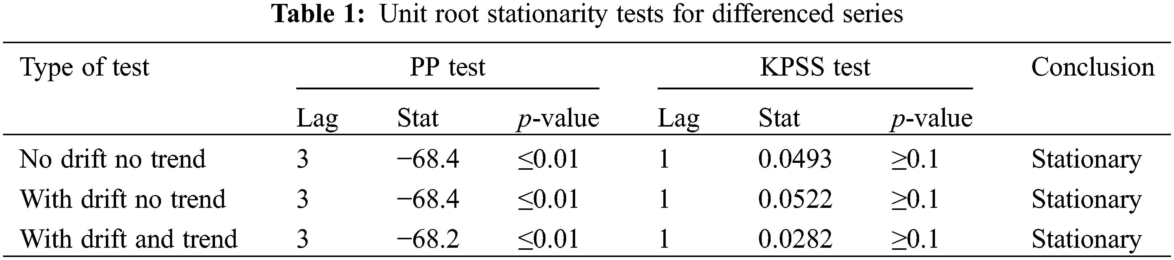
As illustrated in Table 1, the PP test p-values of differenced series under three test types are all ≤0.01, and p-values of KPSS test are all ≥0.1, which indicates that the differenced series is significantly stationary. This conclusion is further confirmed by the rapid decay to within ±2 standard deviations of the sample ACF shown in Fig. 5.

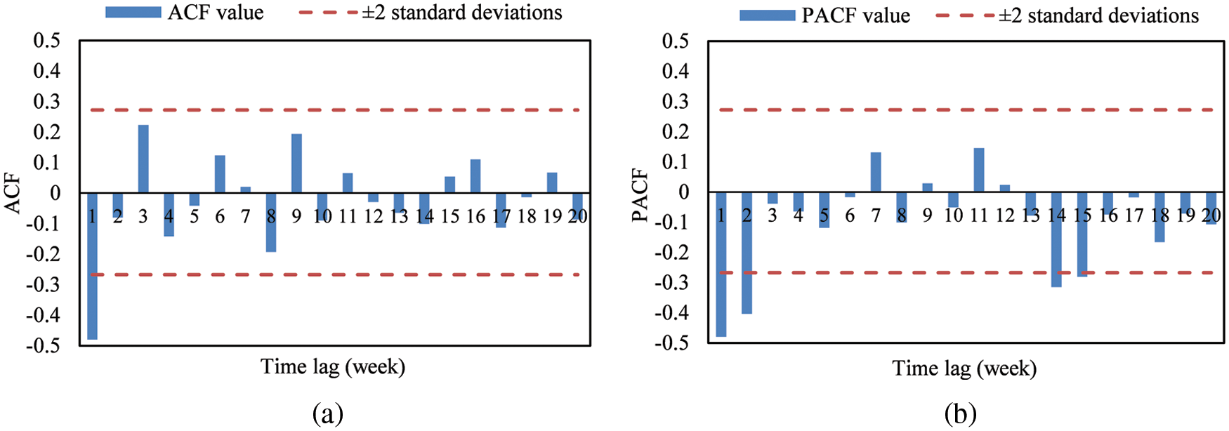
Figure 5: Sample ACF and PCF of differenced series: (a) Sample ACF; (b) Sample PACF

The values of orders p and q can be preliminarily identified by the characteristics of sample ACF (Auto Correlation Function) and PACF (Partial Auto Correlation Function) [38]. Table 2 summarizes the behavior of ACF and PACF for selecting p and q.

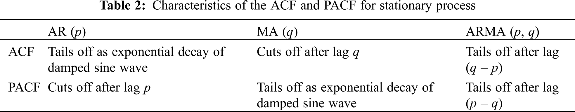
From Table 2, it seems clear that when the ACF or PACF possesses the cutting-off behavior, the identification of the order p of an AR model and the order q of an MA model is relatively simple. For a mixed AR-MA model, however, the ACF and PACF all exhibit tapering off property, which makes the identification of the orders p and q much more difficult. For more complicated models, Tsay et al. [39] introduced the ESACF (Extended Sample Autocorrelation Function) to estimate the orders p and q. In the ESACF table, an ARMA (p, q) will have a pattern of a triangle of zeros, with the upper left-hand vertex at the (p, q) position. However, in the actual identification process, the characteristics of ACF, PACF or ESACF are not always so clear-cut. Therefore, multiple possible models are normally picked according to pertinent information, and the model, of which the statistical indicator is in line with the evaluation criteria, is finally selected. The sample ACF and PCF are plotted in Fig. 5. Table 3 shows the ESACF with indicator symbols.

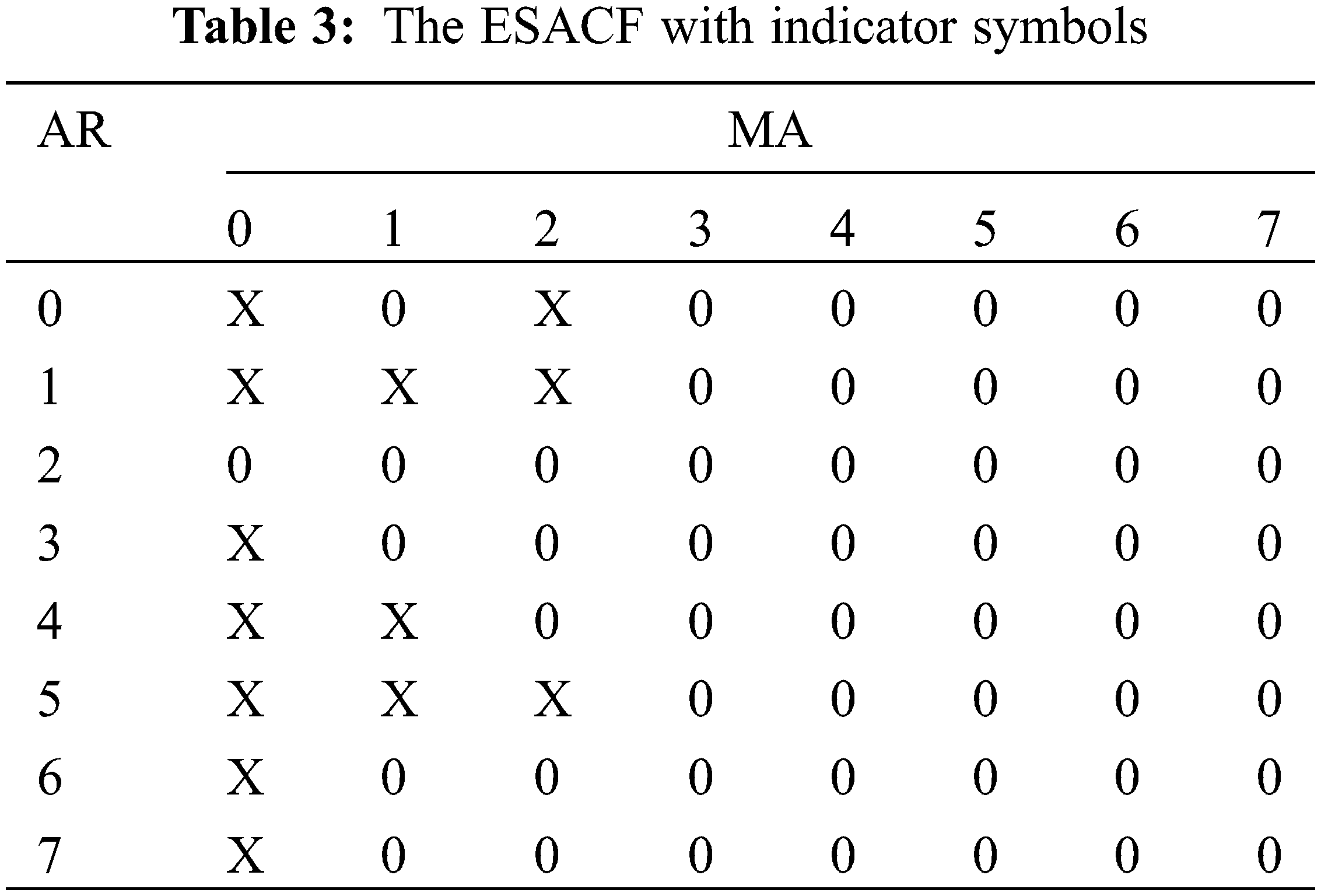
Note from Fig. 5 that the sample ACF exhibits an alternating decreasing pattern and the sample PACF cuts off after lag 2. In the ESACF, the vertex of the zero triangles is located at the (2, 0) position. All these above give a preliminary indication of an ARIMA (2, 1, 0) × (0, 1, 0)48 model. In addition, several adjacent models are also considered. After eliminating the models with insignificant parameters, four adequate models are finally retained for further optimization, which are ARIMA (2, 1, 0) × (0, 1, 0)48, ARIMA (0, 1, 1) × (0, 1, 0)48 and sparse parametric models ARIMA (1, 1, (2)) × (0, 1, 0)48 and ARIMA (1, 1, (2, 3)) × (0, 1, 0)48.

To quantitatively evaluate the accuracy and stability of the preliminary proposed models, the residual sum of squares (RSS), sigma2 ( σ^ε2 ), log likelihood ( ln⁡L^ ), Akaike’s Corrected Information Criterion (AICc), Bayesian Information Criterion (BIC), adjusted R-squared ( R¯2 ) are utilized for model selection [33]. The calculation formulas are shown as follows:

RSS=∑t=1nεt2=∑t=1n(yt−y^t)2 (26)

σ^ε2=RSSn−p−(p+q+1) (27)

ln⁡L^=−n2ln⁡σ^ε2−n2(1+ln⁡2π) (28)

AICc=AIC+2(m+1)(m+2)n−m−2,AIC=−2ln⁡L^+2m (29)

BIC=−2ln⁡L^+mln⁡n (30)

R¯2=1−RSS/(n−m−1)TSS/(n−1),TSS=∑t=1n(yt−y¯)2 (31)

where yt is the observed series; y^t is the predicted value of yt; εt is the residual series; n is the effective number of observations; m is the number of parameters in the model; TSS represents the total sum of squares and y¯ denotes the sample mean.

These statistics are normally based on summary statistics from residuals computed from the fitted model. For RSS, sigma2, log likelihood, AICc and BIC, lower values specify a better model. Adjusted R-squared values range from 0 to 1. A higher adjusted R-squared value closer to 1 indicates a superior. The statistics of the four models are estimated in Table 4.

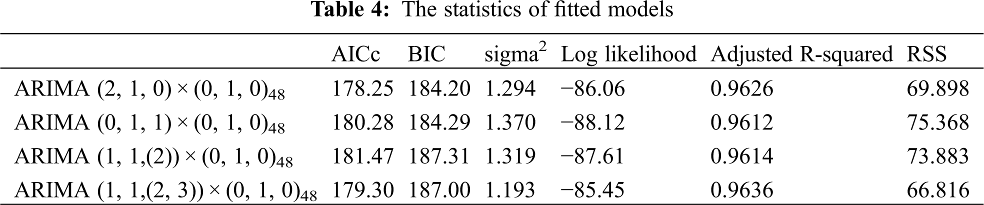
According to the statistical information illustrated in Table 4, the ARIMA (2, 1, 0) × (0, 1, 0)48 model gives the smallest values of AICc and BIC among the four models chosen, while the optimal sigma2, Log likelihood, Adjusted R-squared and RSS indices are coming from the ARIMA (1, 1, (2, 3)) × (0, 1, 0)48 model. After comprehensive comparisons, the relatively concise model ARIMA (2, 1, 0) × (0, 1, 0)48 is selected for final data fitting. The estimation of this model gives

(1−B)(1−B48)yt=εt1+0.6896B+0.4919B2,Var(εt)=1.294 (32)

Fig. 6 gives the residual ACF and the Ljung-Box Q (LB-Q) statistics. Results show that the residual ACFs are all within ±2 standard deviations, and the p-values of LB-Q statistics are all >0.05, which indicates no relevant information is contained in the residuals any longer and the residual series is a white noise process. Thus, the fitted model ARIMA (2, 1, 0) × (0, 1, 0)48 is judged adequate for the data.

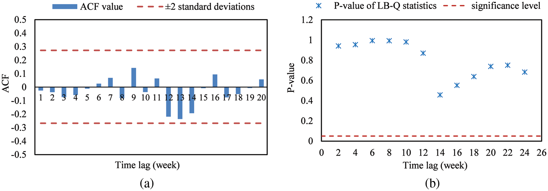
Figure 6: Model adequacy checking results: (a) Residual ACF; (b) p-value of LB-Q statistics

4.3 Detection of Outliers

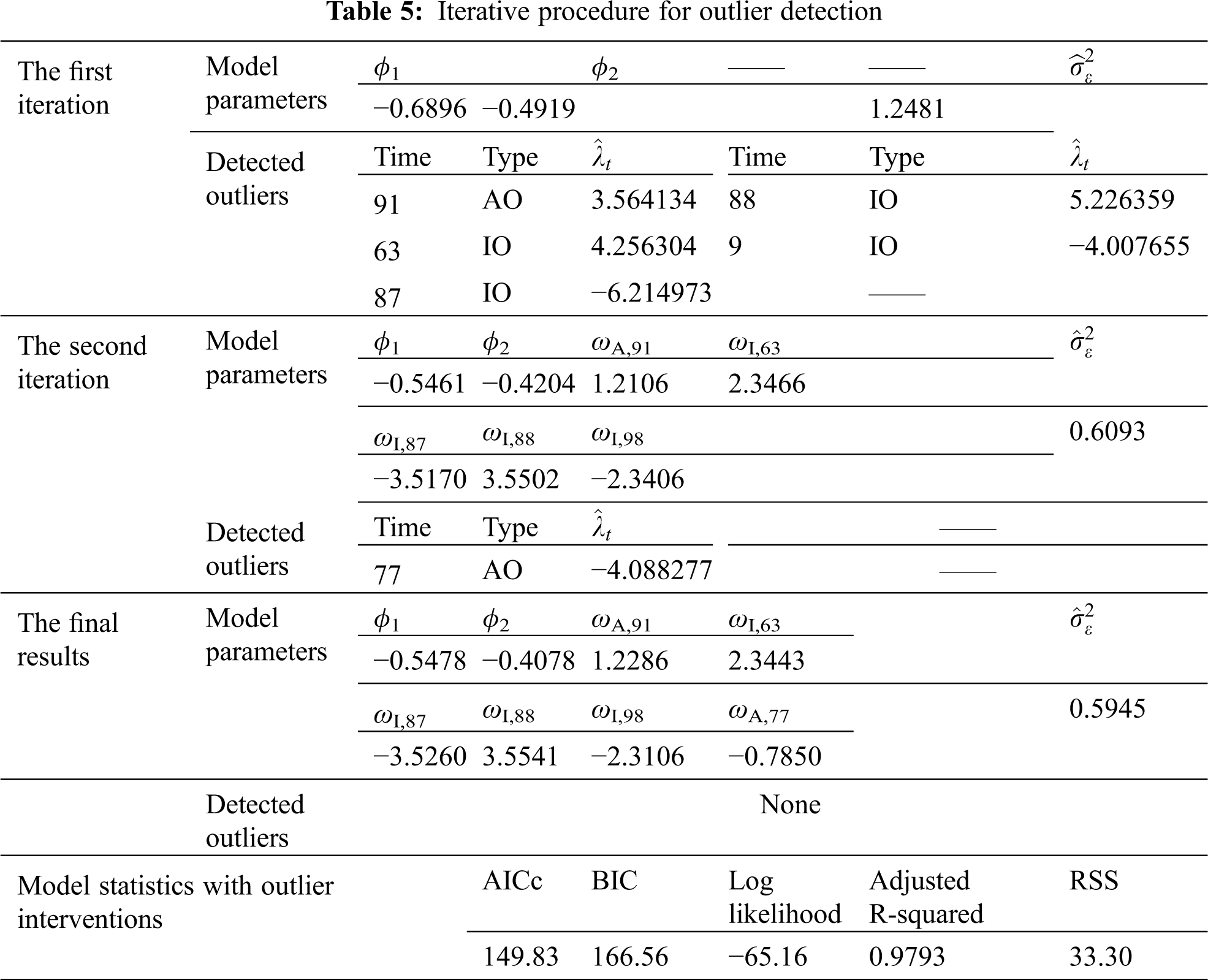
The residual series of the fitted model (see Eq. (26)) is plotted in the legend “Residual of the original model” of Fig. 7. The outlier detecting procedure is then carried out on this residual series. The robust estimator is adopted for the standard deviation of the residuals with the critical value c = 3.5. As a result, a total of 2 AOs and 4 IOs are identified at the significance level 5%, as shown in Fig. 7. The iterative procedure for outlier detection and the details of outliers are listed in Table 5.

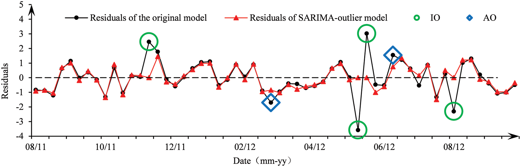
Figure 7: Residual series before and after the identification of outliers

The fitted SARIMA-outlier model can be presented as follows in the form of the main SARIMA model plus outlier interventions:

yt=1(1−B)(1−B48)(1+0.5478B+0.4078B2)×[2.3443Pt(63)−3.5260Pt(87)+3.5541Pt(88)−2.3106Pt(98)+εt]−0.7850Pt(77)+1.2286Pt(91) (33)

After two rounds of iteration, as shown in Table 5, no new outliers are identified. The recognized 2 AOs are from time 77 and 91, and the 4 IOs come from times 63, 87, 88, and 98, respectively. The model parameters ϕ change a lot after the adjustment of outliers on the premise of not changing the structure and the order of the fitted model. The value of σ^ε2 is reduced by about 50%, and other statistics, such as AICc, BIC, RSS, etc., are all optimized greatly. The comparison of the model residuals before and after outlier elimination is illustrated in Fig. 7. It can be seen that the residuals of the two models are basically the same at most of the time points. In the region close to the outliers, the residuals of the SARIMA-outlier model are obviously smaller than those of the original model, and thus σ^ε2 gets a significant decrease, indicating that the adjustment of outliers has a significant impact on the model fitted results. The precision of model fitting improves after including the intervention influence of outliers.

The fitted results of the original model and SARIMA-outlier model are illustrated in Fig. 8 (Note: the first 51 data of the fitted curve are lost due to the differences). Compared with the original model, the SARIMA-outlier model shows a better fitting performance.

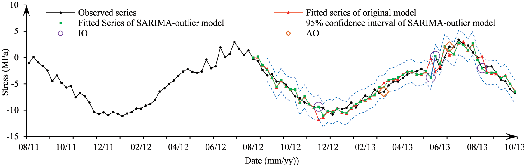
Figure 8: Comparison of the fitted models

4.4 Forecasting Results and Discussion

Use the original model (Eq. (26)) and the SARIMA-outlier model (Eq. (27)) respectively to forecast the weekly mean stress values of measuring point S1.2 in the next 8 weeks. The prediction results are shown in Fig. 9, and the comparison of the accuracy measurement indices of the prediction errors of the two models is presented in Table 6.

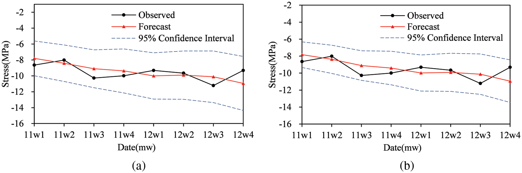
Figure 9: Results of the forecast: (a) Forecasts of the original model (Eq. (26)); (b) Forecasts of the SARIMA-outlier model (Eq. (27))

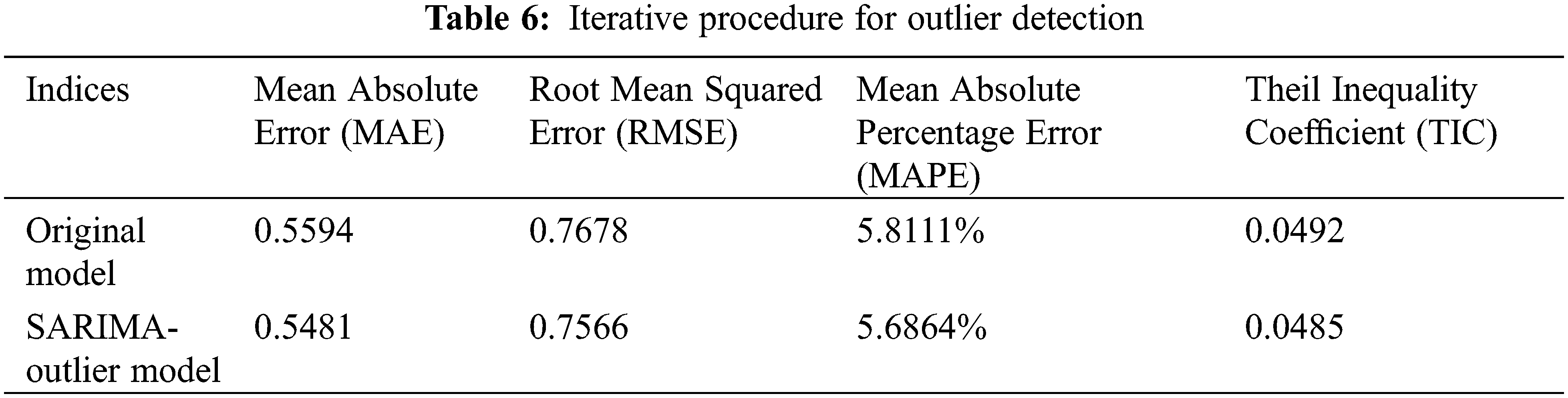
As can be seen from Fig. 9, the width of the 95% confidence interval for the prediction values gradually grows in a trumpet shape, indicating a gradual decrease in the reliability of the prediction. Compared with the original model, the 95% prediction confidence interval of the SARIMA-outlier model is narrower, that is, the prediction reliability remains at a higher level. In terms of the accuracy measurement indices of the prediction errors (see Table 6), the indices of the SARIMA-outlier model are smaller, which also shows a better prediction accuracy. In view of the absolute error of the forecasts, errors of the short-term forecast results fluctuate within a reasonable range, which can meet the needs of forecasts and assessment of bridge structures.

On the other hand, the difference between the predicted values of the two models at each time point is not significant, and the maximum absolute value of the difference is only 0.036. The overall prediction results of the two models are quite close. Therefore, although the existence of outliers has a significant impact on the parameter identification and fitted precision of the time series models, it is insensitive to the forecasting results when there are only a small number of outliers and the value of outlier effect λ is not big. The original model is of strong robustness.

5  Conclusions

In order to ensure the reliability of monitoring data and improve the accuracy of forecasts, the time series model with outliers for bridge monitoring is established using the intervention analysis theory. IOs and AOs are diagnosed and extracted from observed data. Through comparative analysis with the original model without considering outliers, some conclusions are drawn as follows:

(1)   The additive seasonal ARIMA model is suitable for the fitting of bridge monitoring data with obvious seasonal effects. The residuals of the fitted model are white noise, which indicates that the fitted model is of significant effectiveness. Use this model for forecasts, the errors of which can meet the demand for prediction and assessment of bridge structures.

(2)   The outlier detection algorithm presented can rapidly and efficiently identify the outliers existing in BHM data. The detected IOs and AOs are sensitive to the model parameter estimation. After considering the influence of IOs and AOs, the model parameters vary greatly and the fitting accuracy improves significantly, which also verifies the effectiveness and accuracy of the outlier identification.

(3)   In comparison with the original model, the prediction confidence interval of the SARIMA-outlier model is narrower, indicating a more reliable forecasting result. In the meantime, the accuracy measurement indices are smaller and the prediction accuracy is higher.

(4)   The existence of outliers is insensitive to the forecasting results under the condition that the number of outliers is small and the test statistics for outlier effects are not big. The original time series model has strong prediction robustness.

Funding Statement: This work was funded by the Natural Science Foundation of Fujian Province (Grant No. 2020J05207), Fujian University Engineering Research Center for Disaster Prevention and Mitigation of Engineering Structures along the Southeast Coast (Grant No. JDGC03), Major Scientific Research Platform Project of Putian City (Grant No. 2021ZP03), and Talent Introduction Project of Putian University (Grant No. 2018074).

Conflicts of Interest: The authors declare that they have no conflicts of interest to report regarding the present study.

References

1. Flah, M., Nunez, I., Ben Chaabene, W., Nehdi, M. L. (2021). Machine learning algorithms in civil structural health monitoring: A systematic review. Archives of Computational Methods in Engineering, 28(4), 2621–2643. DOI 10.1007/s11831-020-09471-9. [Google Scholar] [CrossRef]
2. Sony, S., Laventure, S., Sadhu, A. (2019). A literature review of next-generation smart sensing technology in structural health monitoring. Structural Control and Health Monitoring, 26(3), e2321. DOI 10.1002/stc.2321. [Google Scholar] [CrossRef]
3. Entezami, A., Sarmadi, H., Behkamal, B., Mariani, S. (2020). Big data analytics and structural health monitoring: A statistical pattern recognition-based approach. Sensors, 20(8), 2328. DOI 10.3390/s20082328. [Google Scholar] [CrossRef]
4. Bao, Y., Chen, Z., Wei, S., Xu, Y., Tang, Z. et al. (2019). The state of the art of data science and engineering in structural health monitoring. Engineering, 5(2), 234–242. DOI 10.1016/j.eng.2018.11.027. [Google Scholar] [CrossRef]
5. Cai, G., Mahadevan, S. (2018). Big data analytics in uncertainty quantification: Application to structural diagnosis and prognosis. ASCE-ASME Journal of Risk and Uncertainty in Engineering Systems, Part A: Civil Engineering, 4(1), 04018003. DOI 10.1061/AJRUA6.0000949. [Google Scholar] [CrossRef]
6. Tu, C. F., Liu, Z. J., Zhang, G., Zhou, L. C., Chen, Y. T. et al. (2017). Processing technique and application of big data oriented to long-term bridge health monitoring. Journal of Experimental Mechanics, 32, 652–663. DOI 10.7520/1001-4888-17-309. [Google Scholar] [CrossRef]
7. Wang, Y., Wang, P., Tang, H., Liu, X., Xu, J. et al. (2021). Assessment and prediction of high speed railway bridge long-term deformation based on track geometry inspection big data. Mechanical Systems and Signal Processing, 158, 107749. DOI 10.1016/j.ymssp.2021.107749. [Google Scholar] [CrossRef]
8. Xu, S., Ma, R., Wang, D., Chen, A., Tian, H. (2019). Prediction analysis of vortex-induced vibration of long-span suspension bridge based on monitoring data. Journal of Wind Engineering and Industrial Aerodynamics, 191, 312–324. DOI 10.1016/j.jweia.2019.06.016. [Google Scholar] [CrossRef]
9. Sun, L., Shang, Z., Xia, Y. (2019). Development and prospect of bridge structural health monitoring in the context of big data. China Journal of Highway and Transportation, 32(11), 1–20. DOI 10.19721/j.cnki.1001-7372.2019.11.001. [Google Scholar] [CrossRef]
10. Sun, L., Shang, Z., Xia, Y., Bhowmick, S., Nagarajaiah, S. (2020). Review of bridge structural health monitoring aided by big data and artificial intelligence: From condition assessment to damage detection. Journal of Structural Engineering, 146(5), 04020073. DOI 10.1061/(ASCE)ST.1943-541X.0002535. [Google Scholar] [CrossRef]
11. Ye, X. W., Jin, T., Yun, C. B. (2019). A review on deep learning-based structural health monitoring of civil infrastructures. Smart Structures and Systems, 24(5), 567–585. DOI 10.12989/sss.2019.24.5.567. [Google Scholar] [CrossRef]
12. Dang, H. V., Raza, M., Nguyen, T. V., Bui-Tien, T., Nguyen, H. X. (2021). Deep learning-based detection of structural damage using time-series data. Structure and Infrastructure Engineering, 17(11), 1474–1493. DOI 10.1080/15732479.2020.1815225. [Google Scholar] [CrossRef]
13. Lara-Benítez, P., Carranza-García, M., Riquelme, J. C. (2021). An experimental review on deep learning architectures for time series forecasting. International Journal of Neural Systems, 31(3), 2130001. DOI 10.1142/S0129065721300011. [Google Scholar] [CrossRef]
14. Faloutsos, C., Gasthaus, J., Januschowski, T., Wang, Y. (2018). Forecasting big time series: Old and new. Proceedings of the VLDB Endowment, 11(12), 2102–2105. DOI 10.14778/3229863.3229878. [Google Scholar] [CrossRef]
15. Oh, B. K., Glisic, B., Kim, Y., Park, H. S. (2019). Convolutional neural network-based wind-induced response estimation model for tall buildings. Computer-Aided Civil and Infrastructure Engineering, 34(10), 843–858. DOI 10.1111/mice.12476. [Google Scholar] [CrossRef]
16. Peng, H., Yan, J., Yu, Y., Luo, Y. (2021). Time series estimation based on deep learning for structural dynamic nonlinear prediction. Structures, 29, 1016–1031. DOI 10.1016/j.istruc.2020.11.049. [Google Scholar] [CrossRef]
17. Zheng, Q. Y., Zhou, G. D., Liu, D. K. (2021). Method of modeling temperature-displacement correlation for long-span arch bridges based on long short-term memory neural networks. Engineering Mechanics, 38(4), 68–79. DOI 10.6052/j.issn.1000-4750.2020.05.0323. [Google Scholar] [CrossRef]
18. Gul, M., Catbas, F. N. (2011). Damage assessment with ambient vibration data using a novel time series analysis methodology. Journal of Structural Engineering, 137(12), 1518–1526. DOI 10.1061/(ASCE)ST.1943-541X.0000366. [Google Scholar] [CrossRef]
19. Pan, H., Lin, Z., Gui, G. (2019). Enabling damage identification of structures using time series–based feature extraction algorithms. Journal of Aerospace Engineering, 32(3), 04019014. DOI 10.1061/(ASCE)AS.1943-5525.0000978. [Google Scholar] [CrossRef]
20. Buckley, T., Pakrashi, V., Ghosh, B. (2021). A dynamic harmonic regression approach for bridge structural health monitoring. Structural Health Monitoring, 20(6), 3150–3181. DOI 10.1177/1475921720981735. [Google Scholar] [CrossRef]
21. van Le, H., Nishio, M. (2015). Time-series analysis of GPS monitoring data from a long-span bridge considering the global deformation due to air temperature changes. Journal of Civil Structural Health Monitoring, 5(4), 415–425. DOI 10.1007/s13349-015-0124-9. [Google Scholar] [CrossRef]
22. Zhu, L., Zhuo, J., Xing, S. (2020). Strain prediction of bridge structural health monitoring based on CEEMDAN-NAR-ARIMA combination model. Science Technology and Engineering, 20(4), 1639–1644. [Google Scholar]
23. Ahmadivala, M., Sawicki, B., Brühwiler, E., Yamalas, T., Gayton, N. et al. (2019). Application of time series methods on long-term structural monitoring data for fatigue analysis. SMAR 2019-5th International Conference on Smart Monitoring, Assessment and Rehabilitation of Civil Structures, pp. 1–8. Postdam, Germany. [Google Scholar]
24. Xin, J., Zhou, J., Yang, S. X., Li, X., Wang, Y. (2018). Bridge structure deformation prediction based on GNSS data using kalman-ARIMA-GARCH model. Sensors, 18(1), 298. DOI 10.3390/s18010298. [Google Scholar] [CrossRef]
25. Shi, H., Worden, K., Cross, E. J. (2019). A cointegration approach for heteroscedastic data based on a time series decomposition: An application to structural health monitoring. Mechanical Systems and Signal Processing, 120, 16–31. DOI 10.1016/j.ymssp.2018.09.036. [Google Scholar] [CrossRef]
26. Jiang, L., Chen, Z. (2016). Stress analysis for a bridge cable-tower anchorage zone based on the singular spectrum analysis. Henan Science, 34(7), 1107–1113. [Google Scholar]
27. Amezquita-Sanchez, J. P., Adeli, H. (2016). Signal processing techniques for vibration-based health monitoring of smart structures. Archives of Computational Methods in Engineering, 23(1), 1–15. DOI 10.1007/s11831-014-9135-7. [Google Scholar] [CrossRef]
28. Seo, J., Hu, J. W., Lee, J. (2016). Summary review of structural health monitoring applications for highway bridges. Journal of Performance of Constructed Facilities, 30(4), 04015072. DOI 10.1061/(ASCE)CF.1943-5509.0000824. [Google Scholar] [CrossRef]
29. Aljoumani, B., Sànchez-Espigares, J. A., Canameras, N., Josa, R., Monserrat, J. (2012). Time series outlier and intervention analysis: Irrigation management influences on soil water content in silty loam soil. Agricultural Water Management, 111, 105–114. DOI 10.1016/j.agwat.2012.05.008. [Google Scholar] [CrossRef]
30. Kaloop, M. R., Elbeltagi, E., Hu, J. W., Elrefai, A. (2017). Recent advances of structures monitoring and evaluation using GPS-time series monitoring systems: A review. ISPRS International Journal of Geo-Information, 6(12), 382. DOI 10.3390/ijgi6120382. [Google Scholar] [CrossRef]
31. Shan, D., Luo, L., Li, Q. (2020). State-of-the-art review of the bridge health monitoring in 2019. Journal of Civil and Environmental Engineering, 42(5), 115–125. DOI 10.11835/j.issn.2096-6717.2020.109. [Google Scholar] [CrossRef]
32. Musa, Y. (2014). Modeling an average monthly temperature of sokoto metropolis using short term memory models. International Journal of Academic Research in Business and Social Sciences, 4(7), 382–397. DOI 10.6007/IJARBSS/v4-i7/1030. [Google Scholar] [CrossRef]
33. Cryer, J. D., Chan, K. S. (2008). Time series analysis: With applications in R, 2nd ed. New York: Springer. [Google Scholar]
34. Moyo, P., Brownjohn, J. M. (2002). Application of Box-Jenkins models for assessing the effect of unusual events recorded by structural health monitoring systems. Structural Health Monitoring, 1(2), 149–160. DOI 10.1177/1475921702001002003. [Google Scholar] [CrossRef]
35. Tsay, R. S. (1988). Outliers, level shifts, and variance changes in time series. Journal of Forecasting, 7(1), 1–20. DOI 10.1002/for.3980070102. [Google Scholar] [CrossRef]
36. Wei, W. W. S. (2006). Time series analysis univariate and multivariate methods, 2nd ed. Boston, MA: Pearson Addison Wesley. [Google Scholar]
37. Chang, I., Tiao, G. C., Chen, C. (1988). Estimation of time series parameters in the presence of outliers. Technometrics, 30(2), 193–204. DOI 10.1080/00401706.1988.10488367. [Google Scholar] [CrossRef]
38. Shumway, R. H., Stoffer, D. S., Stoffer, D. S. (2016). Time series analysis and its applications: With R Examples, 4th ed. New York: Springer. [Google Scholar]
39. Tsay, R. S., Tiao, G. C. (1984). Consistent estimates of autoregressive parameters and extended sample autocorrelation function for stationary and nonstationary ARMA models. Journal of the American Statistical Association, 79(385), 84–96. DOI 10.1080/01621459.1984.10477068. [Google Scholar] [CrossRef]
Cite This Article
Copyright © 2022 The Author(s). Published by Tech Science Press.
This work is licensed under a Creative Commons Attribution 4.0 International License , which permits unrestricted use, distribution, and reproduction in any medium, provided the original work is properly cited.
Downloads
Citation Tools