Structural Durability & Health Monitoring

DOI: 10.32604/sdhm.2022.018202

ARTICLE

Reconstruction Technology of Flexible Structure Shape Based on FBG Sensor Array and Deep Learning Algorithm

Kelong Huang, Jie Yan, Lei Zhang*, Faye Zhang, Mingshun Jiang and Qingmei Sui

Control Science and Engineering Academy, Shandong University, Jinan, 250012, China
*Corresponding Author: Lei Zhang. Email: drleizhang@sdu.edu.cn
Received: 06 July 2021; Accepted: 29 November 2021

1  Introduction

The flexible plate structure is widely used in the aerospace field. This structure has the characteristics of large span, lightweight, and low rigidity [1]. It is susceptible to vibration and deformation due to the influence of the external environment during the working process, which further affects the safety and stability of the flight system [2,3]. Therefore, the deformation monitoring of aerospace structures is critical, which can effectively improve reliability [4,5]. The camera method is a traditional deformation monitoring technology, which mainly obtains the deformation parameters of the structure by taking an image of the measured structure and then processing the image [6,7]. However, this method has disadvantages such as susceptibility to environmental influences and poor anti-vibration interference. Measuring with resistance strain gauge is to measure the structural strain based on the principle that the resistance value changes with strain by pasting the resistance strain gauge on the structure’s surface. This method has the disadvantages of being susceptible to noise interference and complicated configuration system. Compared with the above methods, fiber grating sensors have the advantages of high sensitivity, lightweight, and anti-noise interference, which are widely used in structural health monitoring [8,9]. At the same time, sensor networks can be constructed with space-division multiplexing and wavelength division multiplexing [10–12]. The sensor network constructed by fiber grating sensors is pasted on the surface of a large flexible structure, and the morphology of the structure can be reconstructed by monitoring the sensor information.

At present, scholars have carried out certain researches on morphological reconstruction methods of large-scale flexible structures. Foss et al. [13] proposed the modal conversion method for the first time, which established the displacement reconstruction equation through structural modal and strain. Static experiments on a supporting plate verify that fewer sensors can obtain a more extensive range of structural deformation [13]. The modal conversion method needs to analyze the modals in all directions of the structure, so the model error has a more significant influence on the effect of the reconstruction algorithm. Tessler et al. [14] proposed the inverse finite element method, which constructed the functional relationship between structural strain and displacement through the principle of variational weighted least squares, realized the transformation of the strain field and the displacement field, and achieved the displacement field reconstruction through experiments. It is challenging to construct their functional relationship for complex structures, so the inverse finite element method is only suitable for more superficial structures. Based on the classical beam theory, Ko et al. [15,16] used a piecewise linear function or a nonlinear function to express the surface strain field of the structure by segmenting the structure at equal intervals and realized the reconstruction of the displacement field of the structure through the displacement distribution function and extended it to different structures. The Ko displacement theory reconstruction method requires many sensors to ensure the accuracy of deformation reconstruction, At the same time, the strain measurement in different directions requires multiple sets of sensors. Zhu et al. proposed a deformation reconstruction algorithm based on curvature information to realize the structural reconstruction of solar panels [17]. The curvature reconstruction method will accumulate the error value in the calculation process, and the reconstruction error is relatively large. Therefore, under the premise of ensuring the accuracy of the reconstruction, the method of structural morphology reconstruction needs to develop in a direction that does not depend on structural attributes. Deformation reconstruction using the neural network method can eliminate the constraints of constructing structural models and complex transformation equations. Baldwin et al. [18] used neural network methods to conduct deformation experiments on unilaterally fixed branch structures and achieved good structural deformation reconstruction results. Mao et al. [19] used a simplified neural network to construct a linear mapping method of strain and displacement and realized the deformation reconstruction of complex flexible structures based on the fiber grating sensor array.

Deep learning originates from the research of artificial neural networks. The concept of deep learning was first proposed by Professor Hinton in 2006 [20]. It can deeply mine the characteristics of data through multiple hidden layers. Its main models include convolutional neural network, recurrent neural network, and recursive neural network [21]. Deep learning is used to approximate a non-linear mapping from input to output to achieve prediction results and has adaptive solid and generalization capabilities. However, the traditional neural network structure will degenerate as the number of layers deepens [22]. Therefore, this article will propose a morphological reconstruction technology based on a deep neural network algorithm of cross-layer connection, which can obtain the deformation by establishing the relationship between the strain and displacement of the structure, which is not affected by the error of the structure model.

The aim of the study reported in this paper was to demonstrate the feasibility of the proposed flexible structure reconstruction algorithm based on an improved neural network. The rest of this paper is organized as follows. The next section describes the strain detection principle of the fiber grating sensor, the improved neural network model, and how to establish the mapping relationship between sensor strain and displacement. The following section of the paper then describes a series of structural deformation tests and structural reconstruction model comparison tests employed to demonstrate the feasibility of the reconstruction algorithm proposed in this paper. The last section opens a brief discussion of possible further improvements of the reconstruction model in this paper and concludes some of the advantages of the model.

2  Deep Learning Reconstruction Algorithm

2.1 Principle of Fiber Bragg Grating Strain Sensing

The grating in the fiber grating sensor can be regarded as a narrow-band filter. When light beams with different wavelengths pass through the fiber grating, they will be reflected if their center wavelength meets the grating conditions; otherwise, they will generally pass through the fiber grating. The peak of the reflected light spectrum appears in the center wavelength region of the grating, which is called the Bragg wavelength [23]. Therefore, the reflected light must follow the Bragg condition, which satisfies the Eq. (1) [24].

λB=2neffΛ (1)

where neff represents the effective refractive index of fiber grating; Λ represents refractive index change period; λB represents the central wavelength of reflected light.

To avoid the influence of temperature on the experimental results, a temperature sensor was arranged at the edge of the sensor network for temperature compensation when building the sensor network. The experimental data shows that the temperature is constant during the experiment, so the influence of temperature on the central wavelength of the fiber grating can be ignored, and the relationship between the change of the central wavelength and the strain can be obtained as Eq. (2) [25]

ε=ΔλB(1−Pe)λB (2)

where Pe and λB are constants. The center wavelength change of the fiber grating has a linear relationship with the axial strain. Therefore, after studying the mapping relationship between strain and displacement, the structural displacement can be calculated by the change in the center wavelength of the sensor.

2.2 Principles of Deep Learning Algorithms

A depth neural network is a non-linear mapping. The neurons in the same layer are not connected, and the neurons in adjacent network layers are fully connected. Suppose the input data is x = {IN1, IN2 ⋅ ⋅ ⋅ INn}, the output data is y = {OUT1, OUT2, OUT3, ⋅ ⋅ ⋅ , OUTm}. The network structure model is shown in Fig. 1. However, as the number of layers increases, the expression ability of this structure will decrease. A neural network with a residual structure can avoid this problem. The residual structure includes the identity branch and the residual branch. When the network reaches the optimum, if it continues to deepen the network, the residual branch parameters will learn to be 0 to prevent model degradation. The residual structure is mostly used in convolutional neural networks. This paper improves the fully connected neural network structure based on the idea of residual learning and proposes a cross-layer connected neural network structure. The improved network structure is shown in Fig. 2. In Fig. 2, f(*) is the feature mapping from layer l − 2 to layer l. As shown in the network structure in Fig. 2, l can be 4 (Hidden layer 3) or 6 (Hidden layer 5).

Figure 1: Conventional deep neural network

Figure 2: Improved structure diagram of deep neural network

A neural network needs an activation function to be able to fit any nonlinear function [26]. The ReLU function alleviates the problem of gradient disappearance, makes the neural network have appropriate sparsity, and improves the network training speed. Its expression is shown in Eq. (3) [27]. Therefore, in the model proposed in this paper, ReLU is used as the activation function, and the normalization layer is added to reduce the mutual influence caused by the uneven data distribution of adjacent layers, enhancing the generalization ability of the network and playing a regularization role [28].

g(x)={xx>00x≤0 (3)

The specific structure of the cross-layer connection is shown in Fig. 3, the identity connection is mainly reflected in the identity branch and activation function. This connection structure is mostly used in convolutional neural networks, and rarely directly applied in artificial neural networks. In this paper, after improving part of the neural network structure to a cross-layer structure, the overall structure model can be regarded as a single hidden layer neural network structure based on adding a cross-layer structure. It can be explained that there must be an error value between the output of the single hidden layer neural network and the real output and adding a cross-layer connection between the hidden layer and the output layer can reduce the error value. Due to the existence of the identity connection, the error value will not further deteriorate after the cross-layer connection is added.

Figure 3: Concrete structure of cross-layer connection

In Fig. 3, xi(i = 1, 2, …, l, …L) is the input of the next layer and the output of the previous layer, h is the output before the activation function, wi(i = 1, 2, …, l, …L) is the weight and bi(i = 1, 2, …, l, …L) is the bias. The expanded form of f(*) after ignoring the conversion parameters during normalization can be expressed as follows:

f(∗)=f(xl−2,{wi},{bi}) (4)

where xl−2 is the input of the layer l − 1,{xi} and {bi} are the weight set and bias set when i = l, l − 1.

As can be seen from Fig. 3, the number of neurons in the l − 2 layer is equal to the number of neurons in the l layer and the corresponding connection weight is 1. The output of the l layer can be expressed as

xl=g(xl−2+h) (5)

h can be expressed as

h=f(xl−2,wl−1,wl,bl−1,bl) (6)

Combining Eqs. (5) and (6) can be obtained

xl=xl−2+f(xl−2,wl−1,wl,bl−1,bl) (7)

Assuming that the network structure has L layers, the output of the L − 1 layer can be expressed as

xL−1=xL−3+f(xL−3,wL−2,wL−1,bL−2,bL−1)=x1+∑j=1L−3f(xj,wj+1,wj+2,bj+1,bj+2) (8)

After adding the cross-layer structure to the single hidden layer neural network structure, the cross-layer structure part only needs to learn the difference between the hidden layer output of the single hidden layer neural network structure and the cross-layer structure output.

Δx=∑j=1L−3f(xj,wj+1,wj+2,bj+1,bj+2) (9)

The output value of the last layer is

xL=wLxL−1+bL (10)

Based on the above formula, the relationship between the input and output of the improved neural network model can be expressed as

y= wL(w1x+b1+Δx)+bL(11)

where x is the input of the first layer.

Suppose the cost function of the network model is

E=12‖y−xL‖=12∑k=1nL(yk−xLk)2 (12)

where y is the expected output value and nL is the number of neurons in the last layer.

The essence of the neural network learning process is to find the appropriate parameters to minimize the cost function. The Adam algorithm uses the first-order momentum to adjust the update direction of the parameters and also uses the second-order momentum to adjust the learning rate of different parameters [29]. Therefore, this paper uses Adam gradient descent algorithm to optimize the parameters of the entire model.

According to the chain derivation rule, the partial derivative of the total error to the weight of the cross-layer structure can be obtained

∂E∂wl=δl+2⋅(1+∂∂xlf(xl,{w},{b}))⋅∂∂wlf(xl−2,{w},{b}) (13)

where δl+2 represents the error generated by the output of the l + 2 layer; the partial derivative of each layer bias can also be obtained according to the chain derivation rule.

In the backpropagation, the gradient descent method is used to update the weight and bias of each layer, so that the error between the output of the network model and the true value is as small as possible.

2.3 Establish the Mapping Relationship between Strain and Displacement

In 2.1, the central wavelength of the fiber grating sensor has a linear relationship with the axial strain, and then the mapping relationship between the axial strain of the sensor and the structural displacement can be established to obtain the displacement information of the structure through the central wavelength of the sensor. This paper uses the deep learning algorithm with the powerful ability to approximate nonlinear functions in 2.2 to establish the mapping relationship between the center wavelength of the sensor and the structural displacement. The center wavelength of the sensor is used as the input of the deep learning algorithm, and the displacement information of the structure is used as the output. The deflection curve method calculates the curvature information of the finite point by establishing the equation between the structural strain and the curvature and then calculates the deflection angle of the corresponding point through the curvature after continuous processing, and finally determines the structural displacement according to the deflection angle. The neural network structure model established in this paper can directly learn the corresponding relationship between the strain and displacement of the structure, without the need to deal with complex processes such as structure curvature and deflection angle. The mapping relationship between structural strain and displacement is shown in Fig. 4.

Figure 4: Mapping diagram of strain and displacement

3  Experimental Verification

3.1 Experimental Procedure

Taking the plate structure as the experimental object, the displacement field of this structure subjected to external load is reconstructed. The experimental flowchart is shown in Fig. 5. First, an intelligent structural strain monitoring system is built based on the fiber Bragg grating sensor array. Based on this system, grouping experiments with different loads are carried out. The plate-shaped structure is loaded by controlling the motor compression spring, and its deformation causes the center wavelength of the fiber grating sensor to change. The wavelength information of the fiber Bragg grating sensor array is transmitted back to the high-precision demodulator for demodulation, and the demodulated information is transmitted to the computer for processing and calculation to obtain the wavelength offset. The wavelength offset is converted into strain information according to Eq. (2). The real deformation of the discrete points of this structure is measured by a dial indicator. Then, the proposed improved neural network reconstruction model is used to train and learn the relationship between the strain and the real deformation of the discrete points of this structure. Finally, the data that the model has not learned is passed into the model to obtain the predicted value of this structural discrete point shape variable. Cubic spline interpolation is used for the predicted value to obtain the deformation of the entire displacement field to obtain a visual reconstruction of this structure.

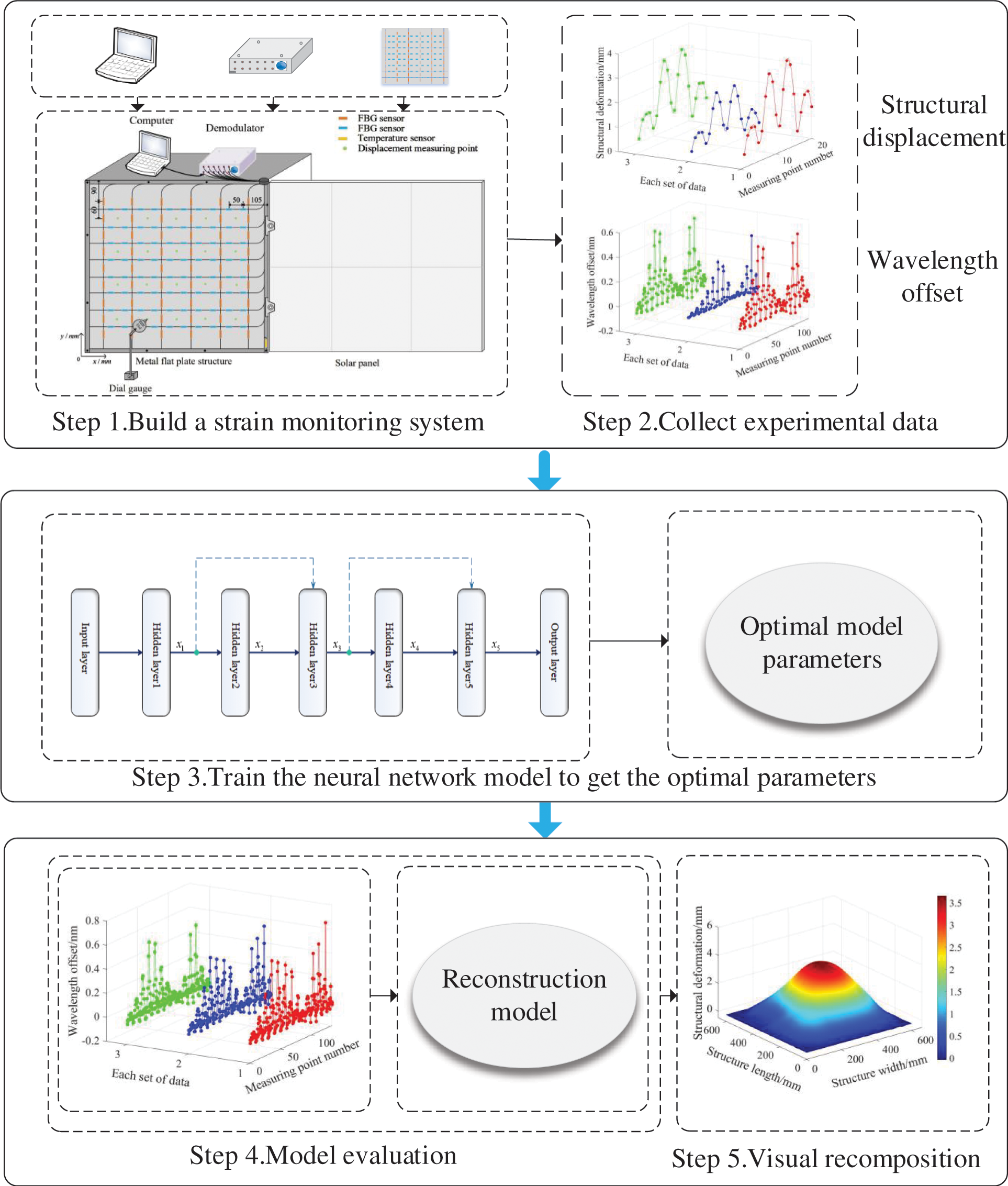
Figure 5: Experimental flow chart

The model diagram of the intelligent structural deformation monitoring system built in this experiment is shown in Fig. 6, mainly composed of a high-density quasi-distributed fiber grating sensing network, a high-precision demodulator dial indicator. The space division multiplexing and wavelength division multiplexing techniques are used to arrange a fiber grating sensor network composed of 14 channels on a plate-shaped structure with a length and width of 600 mm and a thickness of 3 mm. There are 10 sensors in each of the 8 channels of the network, and 9 sensors in each of the other 6 channels. A total of 134 fiber grating sensors are used to collect structural strain information. In addition, a temperature sensor is pasted on the edge of the sensor network to avoid temperature drift. Deploying a high-density quasi-distributed fiber grating sensing network can obtain more detailed information about structural strain. The strain characteristics of the structure learned by the reconstruction model are closer to the actual strain of the entire structure. At the same time, 20 displacement measurement points were selected to measure the real deformation of the discrete points of the structure for later error evaluation.

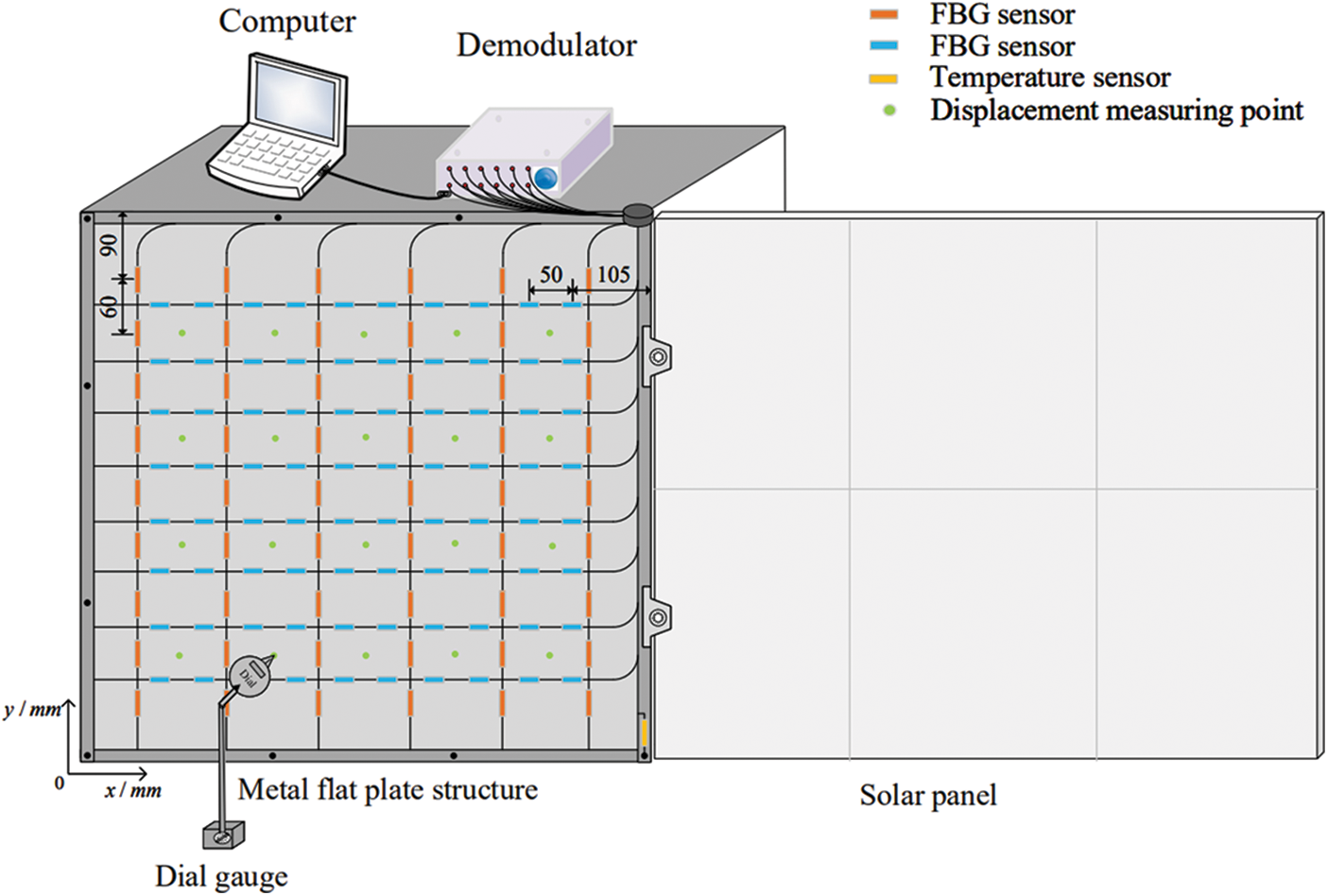
Figure 6: Schematic diagram of test system structure

3.2 Loading Test

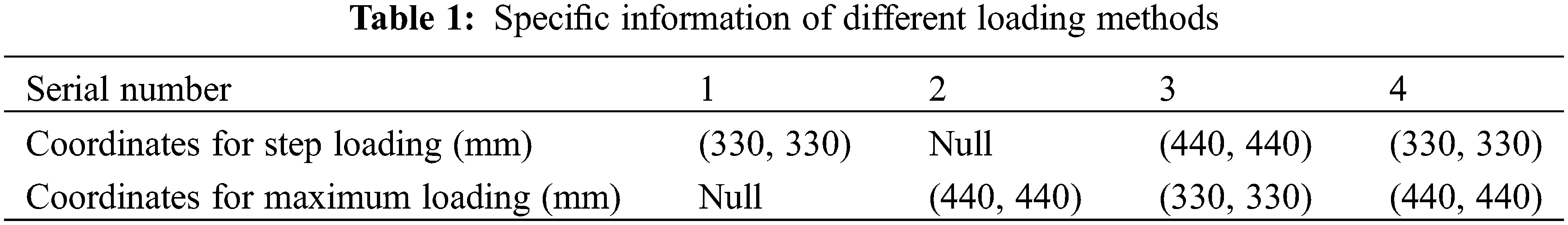
Carry out a loading test on the plate structure, as shown in Fig. 6. The lower-left corner of the plate-like structure is the origin of coordinates. The horizontal direction is the x-axis, and the vertical direction is the y-axis. Four different loading methods are used, as shown in Table 1. The following uses serial numbers 1, 2, 3, and 4 to represent the four methods.

Three sets of experiments were carried out for each loading method, and a total of 120 sample data were collected. The input of the reconstruction model is the structural strain information, and the output is the deformation of the displacement measurement point of the structure. The strain information of the structure can be directly calculated from the center wavelength offset of the sensor network. Some experimental data of the center wavelength offset are shown in Fig. 7. A positive offset indicates that the measuring point is in a stretched state, and a negative offset indicates that the measuring point is in a compressed state. The deformation of the displacement measuring of the structure point is the difference between the indications of the dial indicator.

x=(x11…x1n⋮⋱⋮xm1⋯xmn) (14)

y=(y11…y1n⋮⋱⋮yk1⋯ykn) (15)

where m represents the number of measurement points of the fiber grating sensor; k represents the number of displacement measuring points of the dial indicator; n represents the total number of samples.

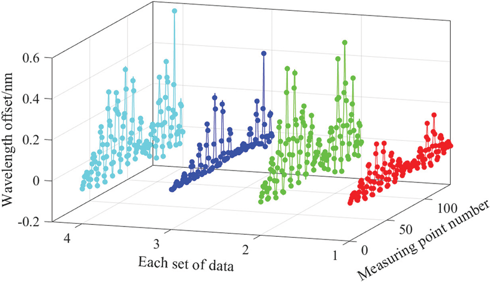
Figure 7: Experimental data of center wavelength offset

3.3 Determining the Number of Hidden Layer Nodes

The network model structure in this paper is composed of a single hidden layer neural network and residual structures. The residual structure is located between the hidden layer and the output layer of the single hidden layer neural network. The network structure is shown in Fig. 3. The number of hidden layer nodes in the network model is related to the mapping ability of the network. When the number of hidden layer nodes is too small, the mapping ability of the network is relatively low, leading to poor results obtained by the model. When the number of hidden layer nodes increases, the mapping ability of the network will improve. However, the time spent in the learning process of the network will also increase, and over-fitting problems may also occur. At present, the academic circles do not have a complete theoretical system to guide the determination of the number of nodes in the hidden layer, and most of them use trial and error methods to determine the final number of nodes in the hidden layer.

In order to evaluate the practical effect of the proposed reconstruction model, the mean absolute error (MAE), the mean square error (MSE), and the average relative error (E) are selected to measure the reconstruction accuracy. Among them, MAE describes the average value of the deviation between the predicted value and the true value, which can well reflect the actual situation of the prediction error. The form of the MSEis the same as the cost function of the reconstructed model, which can well reflect the loss of the model on the test set. The calculation formulas are

MAE=1nk∑i=1n∑j=1k|bij−bij^| (16)

MSE=1nk∑i=1n∑j=1k(bij−bij^)2 (17)

E=1nk∑i=1n∑j=1k|bij−bij^|bij^ (18)

where bij is the predicted value output by the model and b^ij is the expected value of the model output.

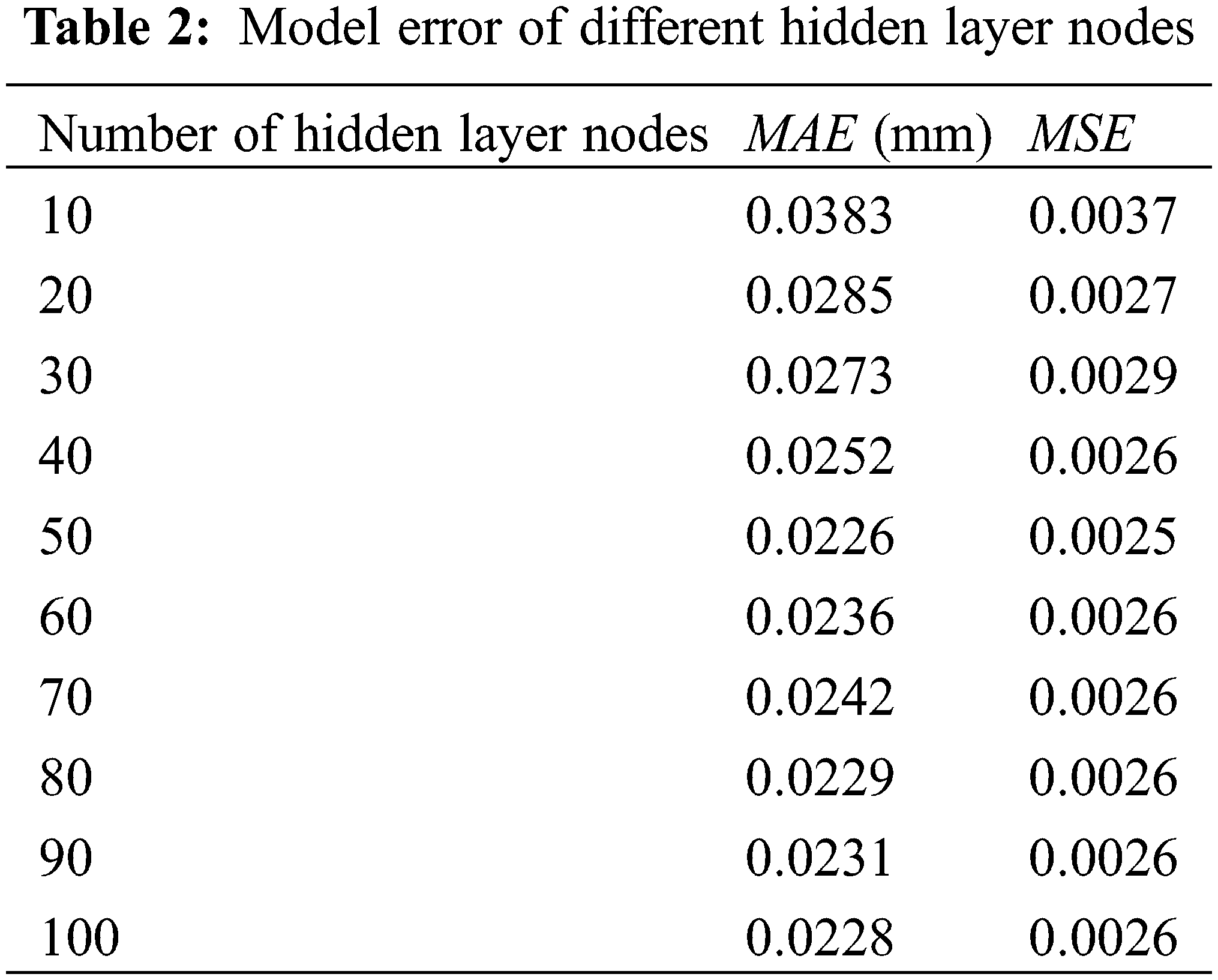
In this paper, the initial value of the number of hidden layer nodes is set to 10, and the number of hidden layer nodes is increased by 10 before the next experiment. To prevent the contingency of the experimental results, each experiment was performed 10 times, and the average of the 10 results was taken as the final result of the experiment. The experimental results are shown in Table 2. When the number of hidden layer nodes is 10–50, as the number of nodes increases, the error of the model continues to decrease; when the number of hidden layer nodes is 50–100, the error of the model is relatively stable and the minimum error is when the number of nodes is 50. Therefore, the number of hidden layer nodes of the network model is determined to be 50 based on the experimental results.

3.4 Model Evaluation

Each group of experimental data is randomly divided into training data and test data at a ratio of 4:1, and there is no duplicate data. In order to observe the reconstruction effect of the improved neural network model proposed in this paper, compare it with decision tree regression and conventional neural network. Classification And Regression Tree (CART) is a kind of decision tree, which can be used to create a classification tree, a regression tree, and a model tree. In this paper, we use CART to build a regression tree with structural strain as input and displacement as output. The variation of the average error value obtained by CART with the depth of the tree is shown in Fig. 8a. It can be seen that the error value reaches the minimum when the depth is 4, so the depth of the tree is selected as 4.

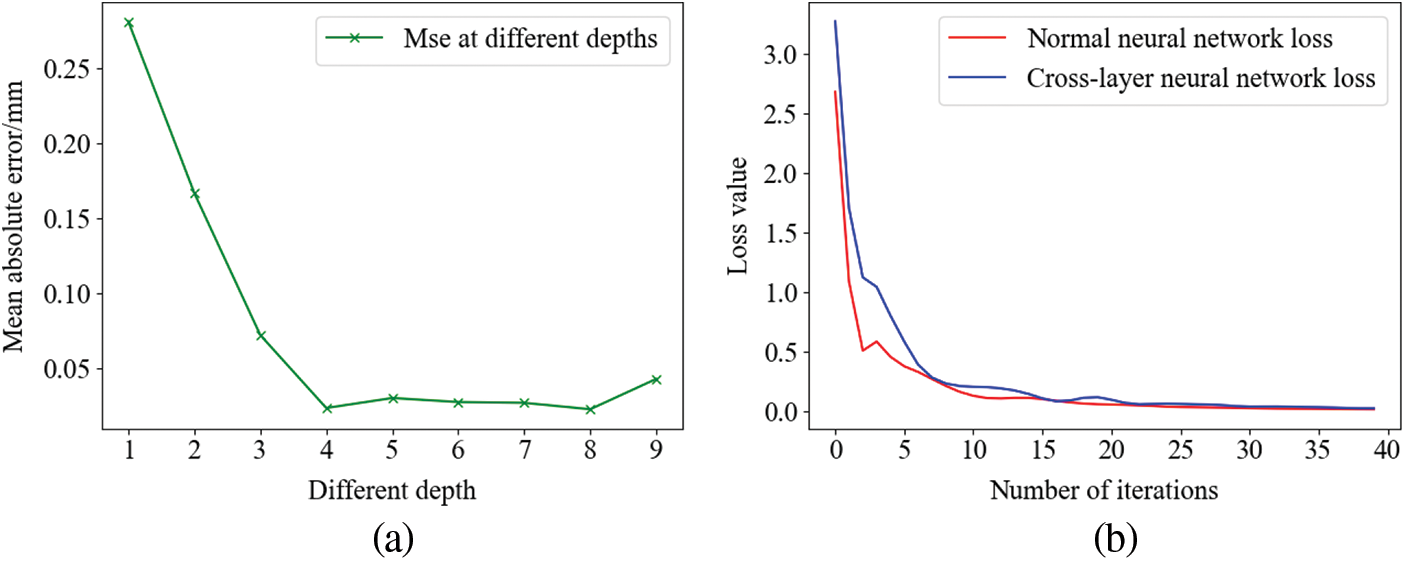
Figure 8: (a) Selection of decision tree depth and (b) Training loss curve of neural network

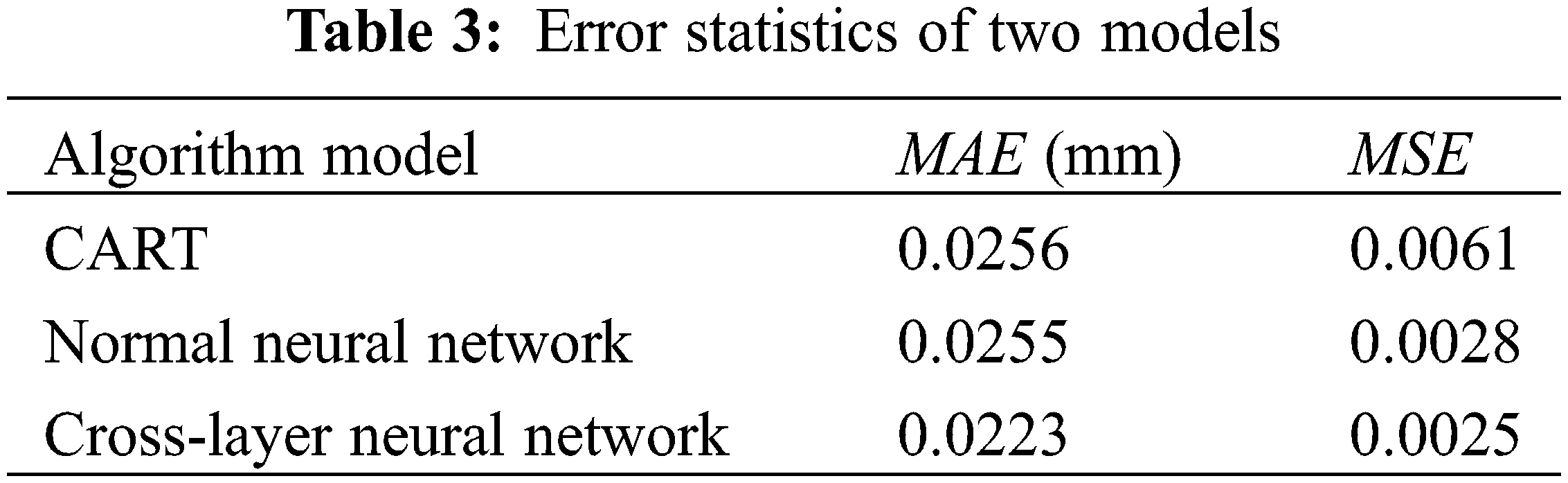
In order to verify the effectiveness and stability of the improved neural network proposed in this paper, the three structural reconstruction methods were trained 50 times, respectively. The network structure is shown in Fig. 4, and the number of hidden layer neurons is 50. Fig. 8b is a graph of the loss curve of the training set during the one-time training process of the conventional neural network and the cross-layer neural network. The MAE and MSE of the 50 times are sorted from small to large, respectively, as shown in Fig. 9, and the total error results are shown in Table 3.

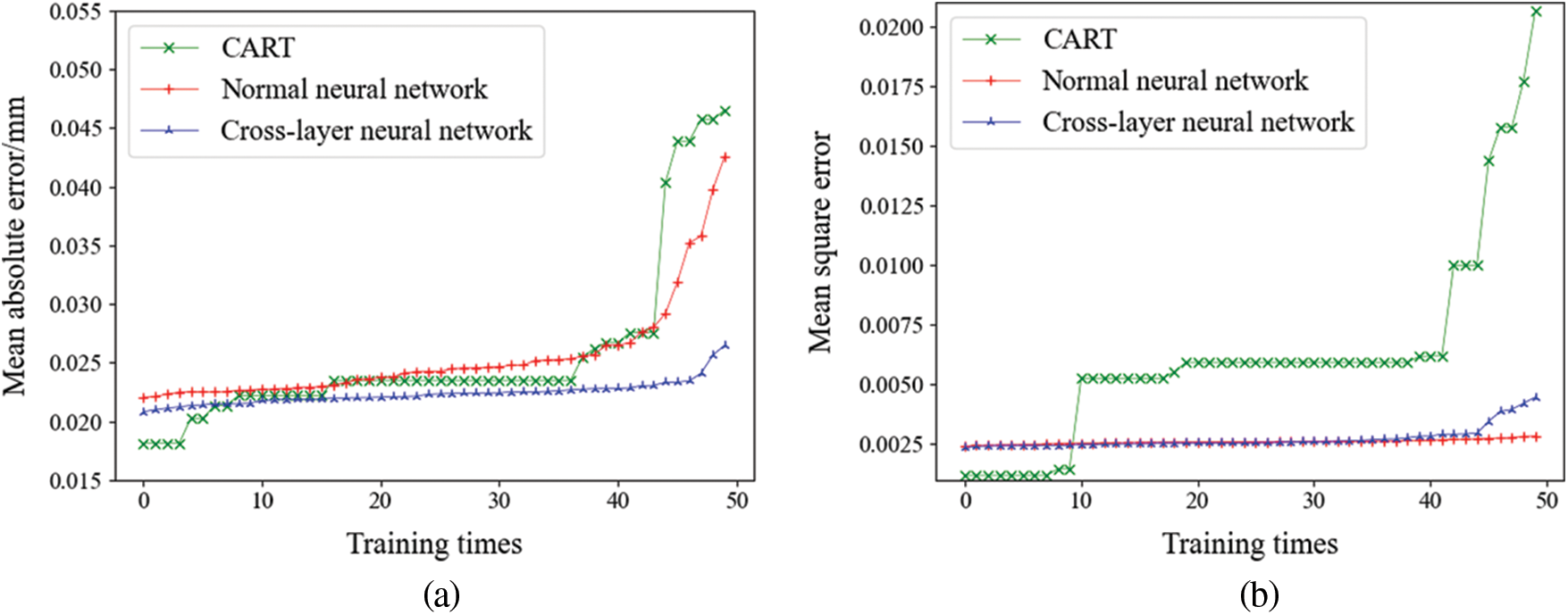
Figure 9: Error statistics for 50 time; (a) MAE and (b) MSE

Define the floating ratio η to evaluate the stability index:

η=emax−e¯e¯×100%(19)

where emax is the maximum error of the sample and e¯ is the average of the sample error.

It can be seen from Table 3 that the MAE of the CART model for 50 times is 0.0256 mm, the maximum value is 0.0465 mm, and the floating ratio is 78.43%. The MAE of 50 times of the conventional neural network model is 0.0255 mm, the maximum is 0.0426 mm, and the floating ratio is 78.43%. The MAE of 50 times of cross-layer neural network model is 0.0223 mm, the maximum is 0.0264 mm, and the floating ratio is 25.11%. It can be seen that the two evaluation indicators of the cross-layer neural network model are better than CART and the conventional neural network model, with high accuracy and more stability.

3.5 Displacement Field Reconstruction

The test data is reconstructed based on three different reconstruction models, and the inversion effect of the displacement field of the structure is experimentally verified. Table 4 shows the average error statistics of the four different loading methods. Fig. 10 shows the reconstruction results of the test data of the second set of experiments under different loading methods and the visualization renderings of the reconstruction results of the cross-layer connection neural network model.

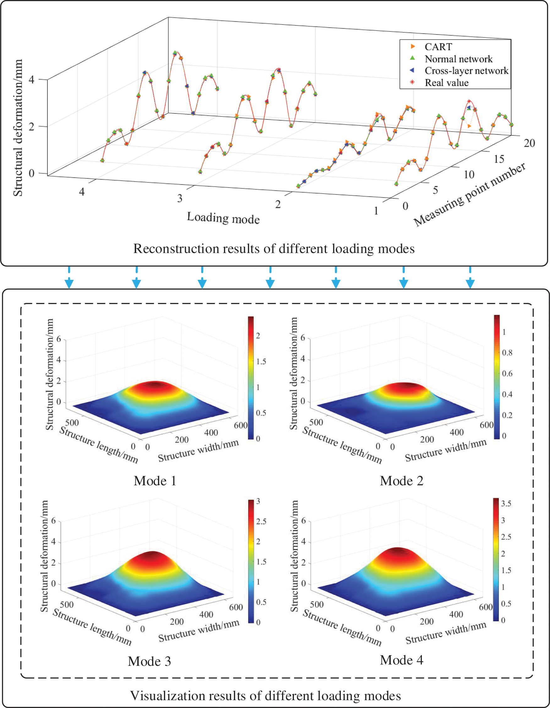
Figure 10: Reconstruction result display

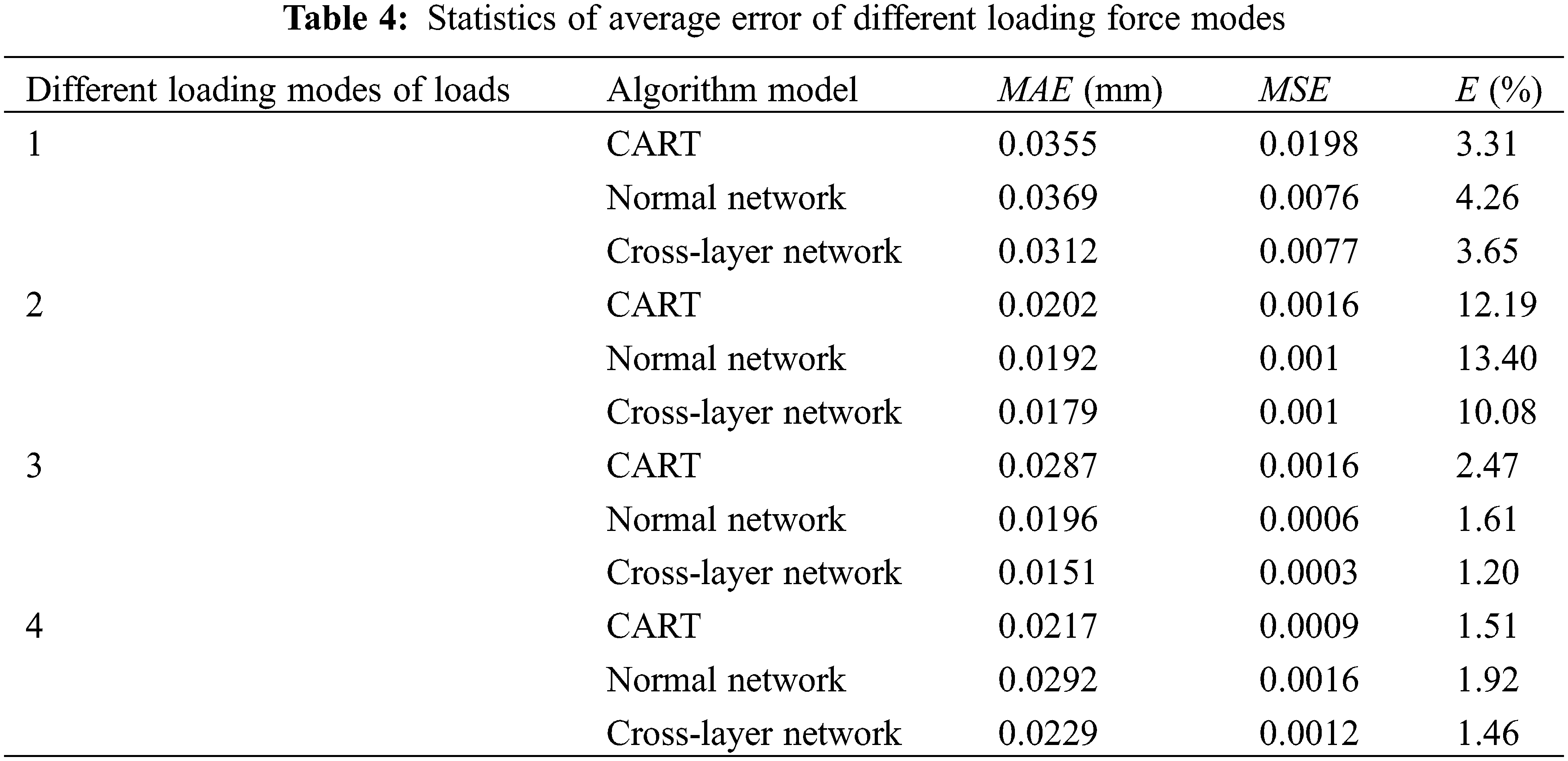
As shown in Table 4, the error of the displacement prediction value of the structure discrete point output by the cross-layer neural network is smaller than CART and the conventional neural network prediction value error under different stress loading conditions. The MAE of the four cases of the cross-layer neural network is 0.0217 mm, which is better than the 0.0265 mm of CART and the 0.0262 mm of the conventional neural network; the E is 4.09%, which is better than the 4.87% of CART and the 5.3% of the conventional neural network. Due to the existence of the identity branch, the cross-layer neural network only needs to learn the difference between input and output instead of directly learning the complex mapping relationship between input and output. This feature makes it easier to learn compared to the original neural network structure. The experimental results show that the MAE of the cross-layer neural network under four different stress conditions is less than 0.032 mm, and all the error indicators are better than the conventional neural network. It is verified that overlaying a cross-layer structure on a single hidden layer network is more effective than simply overlaying a fully connected layer.

4  Discussion

In this paper, an intelligent structural deformation monitoring platform based on the fiber Bragg grating sensor array is built for the flat structure on the aerospace vehicle, and a cross-layer connection deep neural network reconstruction model is proposed. The structure deformation experiments under different stresses are carried out on the platform, and the structure displacement field is reconstructed using the proposed reconstruction model. The novelty of this paper is that the idea of residual learning is applied to the conventional fully connected neural network to obtain an improved neural network structure, and this model is applied to the reconstruction of flexible structures.

Compared with the other traditional structural reconstruction models introduced in the introduction, the reconstruction model proposed in this paper establishes the mapping relationship between structural strain and displacement, and obtains displacement information directly from the collected strain information, without the need to establish complex conversion equations. The experimental results show that the reconstruction algorithm obtained by improving the conventional fully connected neural network based on the idea of residual learning is better than the conventional neural network and decision tree regression algorithm. As shown in the experimental results in Fig. 9, although the reconstruction error of several experiments of the decision tree regression algorithm is better than that of the improved neural network model proposed in this paper, its total average error and overall stability are worse. The limitation of the improved neural network structure is that the number of neurons in the first and last layers of each cross-layer structure is the same so that the output of the first layer can be used as the input of the tail layer. Therefore, we can take the limitation of the number of neurons in the cross-layer structure as the next research question for further research.

5  Conclusions

Based on the conventional neural network, this paper proposes a cross-layer connection neural network reconstruction model based on the idea of residual learning. The reconstruction effect of the cross-layer network model is better than that of CART and conventional neural network, and we can conclude that it has the following advantages:

(1) Higher accuracy and better stability. Compared with the conventional neural network, due to the addition of a cross-layer structure, the learning of the entire network structure is more accessible, and the reconstruction accuracy is improved. In addition, the stability of the learning ability is also improved.

(2) Wider scope of application. The improved deep neural network effectively solves network degradation caused by the superposition of network layers after adding a cross-layer structure. When the measured structure is broad and many fiber Bragg grating sensors are needed for measurement, a more complex network structure is needed to learn the correspondence between strain and displacement. Compared with the conventional neural network structure, the cross-layer connection network structure proposed in this paper is more applicable.

Acknowledgement: The authors are grateful for the financial support provided by National Natural Science Foundation of China, National Key Research and Development Project and Key Research and Development Plan of Shandong Province.

Funding Statement: This work was supported by National Natural Science Foundation of China (61903224, 62073193 and 61873333), National Key Research and Development Project (2018YFE02013) and Key Research and Development Plan of Shandong Province (2019TSLH0301 and 2019GHZ004).

Conflicts of Interest: The authors declare that they have no conflicts of interest to report regarding the present study.

This work is licensed under a Creative Commons Attribution 4.0 International License, which permits unrestricted use, distribution, and reproduction in any medium, provided the original work is properly cited.