Structural Durability & Health Monitoring

DOI: 10.32604/sdhm.2022.019554

ARTICLE

Shape Sensing of Thin Shell Structure Based on Inverse Finite Element Method

Zhanjun Wu1, Tengteng Li1, Jiachen Zhang2, Yifan Wu3, Jianle Li1, Lei Yang1 and Hao Xu1,*

1State Key Laboratory of Structural Analysis for Industrial Equipment, Dalian University of Technology, Dalian, 116024, China
2Division of Science and Technology, Beijing Normal University—Hong Kong Baptist University United International College, Zhuhai, 519000, China
3Country School of Marxism, Northeastern University, Shenyang, 110167, China
*Corresponding Author: Hao Xu. Email: xuhao@dlut.edu.cn
Received: 29 September 2021; Accepted: 22 December 2021

1  Introduction

In the last decades, curved thin-shell structure such as composite tank of spacecraft has been widely used in aerospace because of its excellent bearing capacity and weight-saving [1,2]. Structural integrity is the key factor to ensure its function and strength, but the complex construction process makes it prone to defects. Meanwhile, the tank structure bears time-varying load conditions during service, which may damage its structural integrity and reduce its remaining life. Therefore, the establishment of a health monitoring system for real-time monitoring structural state and predicting damage can play an important role in the whole life cycle of structure manufacturing, service and maintenance. Traditional nondestructive testing technologies such as ultrasonic testing [3,4] and acoustic emission technology [5,6] have the problems of time-consuming and high cost which make it not suitable for real-time monitoring of structural response. So the health monitoring technology based on embedded strain sensors (optical fiber sensors, strain gauges, etc.) will become an important direction of structural health assessment in the future [7,8].

The dynamic reconstruction of the three-dimensional displacement field of a structure known as shape sensing is a crucial component of structural health monitoring which provides data support for subsequent calculation of stress and strain and failure prediction. Furthermore, the real-time evaluation of the deformed shape is also a vital technology for the development of smart structures such as morphed capability and embedded conformal antennas that require real-time shape sensing to provide feedback for their actuation and control systems.

Numerous studies on shape sensing found in the open literature can be divided into the following categories: (1) the Modal Method (MM) [9–12]; (2) analytical methods [13–15]; (3) Artificial Neural Networks (ANN) [16,17]; (4) the inverse Finite Element Method (iFEM) [18–20]. MM, firstly developed by Foss et al. [9], is a modal transformation algorithm in which the displacement field of the structure is expressed by modal shapes and corresponding weights. The modal shapes are known and the weights need to be computed using strain–displacement relationship and measured surface strains. There are two different ways to calculate modal shapes. The first one is to use the finite element method or analytic method, but it requires such prior information as the material properties [11]. The other is to estimate experimentally but it could be significantly onerous [12]. Based on the Bernoulli–Euler beam theory, Ko et al. [13] constructed the displacement transfer function by fitting the axial strain distribution with piecewise polynomials, and further obtained the bending deflection of the beam. However, Ko’s theory only considers simple bending deformation of the beam, and could do nothing about the coupling deformation of beam structures subjected to highly coupled loading cases. Xu et al. [14,15] proposed a novel method that could decouple complex beam deformations subject to the combination of different loading cases, including tension/compression, bending and warping torsion to reconstruct deformed shape of thin-walled beam structures. The ANN needs a large number of parameters, such as network topology, weight and initial value of threshol and a lot of training time. Moreover, ANN can be regarded as a black box and the results calculated are difficult to explain, which will affect the credibility and acceptability of the results. Generally speaking, each of the above methods has certain limitations, so the scope of application is limited.

In order to reconstruct the three-dimensional displacement field in real-time with strain data obtained from the structure surface, Tessler et al. [20] developed an inverse Finite Element Method (iFEM). The iFEM is formulated based on a weighted-least-square error functional between the analytical and experimental values of strain on the structure surface. Like the classic Finite Element Method (FEM), iFEM is also a model-based technique. Therefore, the application of iFEM is not limited by complex boundary geometry and conditions. Moreover, the formulation only makes use of strain-displacements relations which make any information about materials or load acting on the structure is unnecessary. Numerous studies had proved the applicability and robustness of iFEM and different elements such as iMIN3 [20], iQS4 [19], and iCS8 [21] elements and so on had been developed for different application structures. All elements are developed based on Mindlin theory, and interpolated using the anisoparametric shape functions developed by Tessler and Hughes to avoid shear locking when modeling thin shell structures. Though it has achieved good results, the Kirchhoff–Love shell model is well suited for thin shell analysis in fact because it disregards transverse shear deformations which reveals that the deformation of thin shells is physically dominated by membrane and bending actions and the shear locking can be avoided completely.

The main focus of this work is to redefine the weighted-least-square error functional based on classical plate theory. Subsequently, a new four-node quadrilateral inverse-shell element, iDKQ4, is developed for numerical implementation. The new element includes hierarchical drilling rotation degrees-of-freedom (DOF) to enhance applicability in modeling complex structures. This study is organized as follows: the iDKQ4 element is presented in brief in Section 2. Besides, an iFEM formulation developed utilizing the kinematics of Kirchhoff–Love shell theory for thin shells, is introduced. In Section 3, a cantilever plate model is firstly employed to demonstrate the reconstruction performance of the iDKQ4 element. Then a wallpanel is analyzed to demonstrate the robustness for modeling complex shell structures. Finally, the deformation of a typical aerospace thin wall structure (the composite tank) is computed with a few strain data with the help of the iDKQ4 element. The conclusions of this study are provided in Section 4.

2  Inverse Finite Element Formulation for Thin Shells

Consistent with obtaining a flat element formulation, the inverse shell element can also be regarded as a superposition of a plate-bending element and a membrane element. In this paper, the four node plane stress (as shown in Fig. 1a) element and the DKQ plate bending element based on discrete Kirchhoff theory [22] (as shown in Fig. 1b) are selected and add them together to get the inverse shell element iDKQ4 (as shown in Fig. 1c). There are six degrees-of-freedom (DOFs) at each node, as shown in Fig. 1c, where u and v are in plane translations; w is transverse deflection; θx and θy are bending rotations, and θz is in-plane rotation. Due to inclusion of drilling rotations, the adaptability of iDKQ4 element to complex structures is greatly enhanced. Furthermore, the transverse shear is neglected in Kirchhoff–Love shell theory which reveals that the shear locking can be completely avoided.

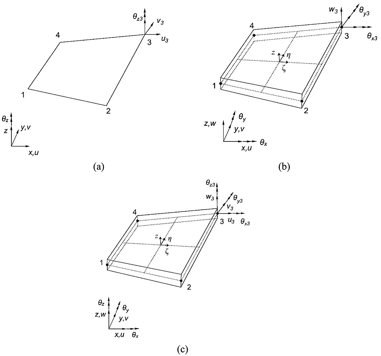
Figure 1: (a) The plane stress element (b) the DKQ plate bending element (c) the iDKQ4 element

The 4-node membrane element with drilling DOFs is derived by combining the in-plane displacements using Allman-type interpolation functions [23,24] with the standard bilinear independent normal (drilling) rotation fields.

u=∑i=14Niui+∑i=14Liθzi (1)

v=∑i=14Nivi+∑i=14Miθzi (2)

where N is the standard bilinear isoparametric function, and L and M are the shape functions that define the interaction between the drilling rotation fields and the displacement of the element membrane. Details of the formulation can be found in the original literature.

At the four corner nodes, two bending rotations θx , θy are the derivatives of the displacement w.

θxi=w,yiθyi=−w,xi (3)

Therefore, these kinematic variables are related using the shape functions developed by Batoz for DKQ element [22]. These interpolations are given as

θx=∑i=14H4i−3xwi+∑i=14H4i−2xθxi+∑i=14H4i−1xθyi (4)

θy=∑i=14H4i−3ywi+∑i=14H4i−2yθxi+∑i=14H4i−1yθyi (5)

From the strain-displacement relationship of linear elastic theory, we can know that

εxx=∂u∂x+z∂θy∂x (6)

εyy=∂v∂y−z∂θx∂y (7)

γxy=∂v∂x+∂u∂y+z(∂θy∂y−∂θx∂x) (8)

γxz=γyz=0 (9)

It should be noted that the plane stress assumption σzz means that the transverse-normal strain εzz has no contribution to the strain energy.

The generalized strains vector consisting of membrane strain e and bending strain k can be defined as

{ε1ε2⋯ε6}={e;k}T (10)

where

e=[ε1,ε2,ε3]=[B1ue,B2ue,B3ue] (11)

κ=[ε4,ε5,ε6]=[B4ue,B5ue,B6ue] (12)

where the node displacement vector of iDKQ4 element can be expressed as ue=[u1e,u2e,u3e,u4e] , and each node contains six degrees of freedom uie=[ui,vi,wi,θxi,θyi,θzi]T (i = 1,…,4). The matrices B contain derivatives of the shape functions, and the explicit expressions are as follows:

Bi=[B1iB2iB3iB4i] (13)

Bj1=[Nj,x0000Lj,x] (14)

Bj2=[0Nj,y000Mj,x] (15)

Bj3=[Nj,yNj,x000Mj,x+Lj,y] (16)

Bj4=[00H4∗j−3,xxH4∗j−2,xxH4∗j−1,xx0] (17)

Bj5=[00H4∗j−3,yyH4∗j−2,yyH4∗j−1,yy0] (18)

Bj6=[00H4∗j−3,xy+H4∗j−3,yxH4∗j−2,xy+H4∗j−2,yxH4∗j−1,xy+H4∗j−1,yx0] (19)

In order to decouple plane strain and curvatures, the strain rosettes need to be attached to the top and bottom surfaces of the element as shown in Fig. 2. The sensor can use traditional strain gauges or fiber-optic sensor such as distributed optical fiber, and optical fiber can collect a large amount of strain data as input for iFEM calculation, which make it more attractive.

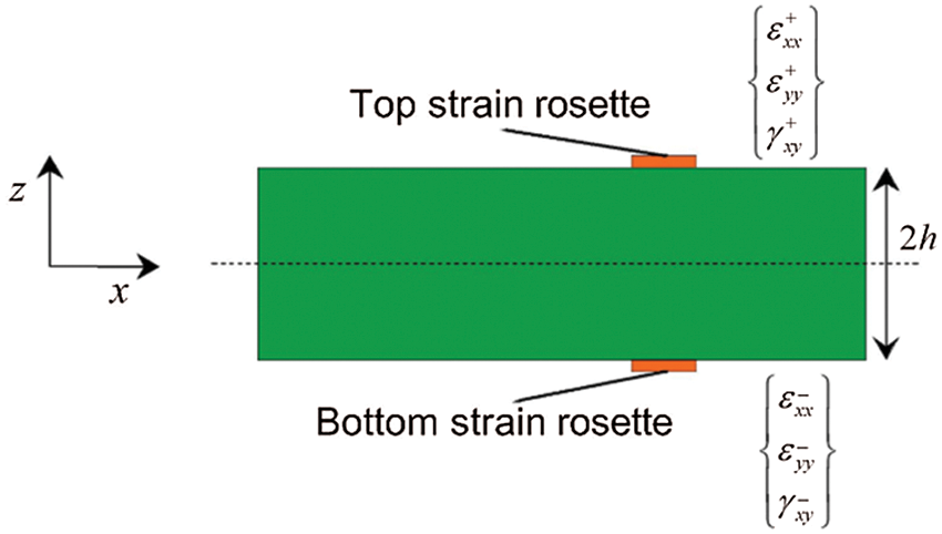
Figure 2: Discrete surface strains measured on the iQS4 element

The counterpart of membrane strains and bending curvatures calculated from Eqs. (11) and (12) can obtain by using the following formula with measured strain data:

eiε≡[ε1εε2εε3ε]=12{εxx++εxx−εyy++εyy−γxy++γxy−} (20)

kiε≡[ε4εε5εε6ε]=12h{εxx+−εxx−εyy+−εyy−γxy+−γxy−} (21)

where {εxx+εyy+γxy+}iT and {εxx−εyy−γxy−}iT are the measured strains on the upper and lower surfaces respectively with the superscripts ‘+’ and ‘−’ denoting the quantities that correspond to the top and bottom surface locations, respectively.

For an individual inverse element, the error functional with respect to DOFs of the entire discretization can be expressed as:

ϕe(ue)=∑k=16wk‖εk(ue)−εkε‖ (22)

where εk(ue) and εkε represent the theoretical strain and the corresponding measured values at a given point respectively. The error function consist with membrane strain, bending strain only which is consistent with the classical plate theory.

The squared norms expressed in Eq. (22) can be written in the form of the normalized Euclidean norms:

‖εk(ue)−εkε‖=1n∫Ae∑i=1n[εk(i)(ue)−εk(i)ε]2dAe (23)

where Ae represents the area of the middle surface of the element and n is the number of measuring points in the element. wk is the weight coefficient that represents the strength of the constraint between the theoretical strain and its corresponding measured value. The specific form is defined by Eq. (24).

{wk}={λ1,λ2,λ3,4h2λ4,4h2λ5,4h2λ6} (24)

If all the values in {εε} can be obtained, the weight coefficient (k = 1,…, 6) is set to 1, otherwise, the corresponding weight coefficient is set to a small value, for example, 10−5 .

Minimizing the error function with respect to the unknown nodal displacement DOF gives rise to

∂ϕe(ue)∂ue=keue−fe=0⇒keue=fe (25)

where ke is only a function of the measuring position. Once the measuring point position is determined, it is determined. fe is a function of the measuring position and the measured strains, which are updated in real-time with the measured strains. The variational statement given in Eq. (25) results in a linear system of equations that can be solved for the unknown DOF provided that appropriate displacement boundary conditions have been imposed.

3  Numerical Validation

3.1 A cantilever Plate under Static Transverse Force Near Free Tip

Firstly, the cantilever plate model is used to verify the accuracy of iDKQ4 element. As shown in Fig. 3, the dimension of the cantilever plate is 254 × 76.2 × 3.175 mm. The material is aluminium alloy (with Young’s modulus of 73.084 GPa, Poisson’s ratio of 0.33 and density of 2700 kg/m3). A concentrated force of 25.728 n is applied along the negative direction of the z-axis near the tip. Bogert et al. [11] initially analyzed the plate and then tested it in the mechanics laboratory. Then, Tessler et al. [25] analyzed this structure using iFEM method with iMIN3 element. Kefal et al. [19] also adopted iFEM method to reconstructed the displacement field of this structure with iQS4 element to verify its bending performance.

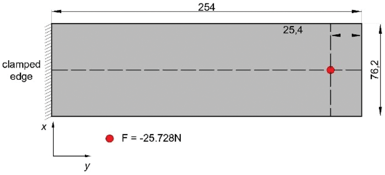
Figure 3: Cantilever plate under transverse force applied near free tip

In order to validate the bending capability of iDKQ4 element, the cantilever plate is discretized with 28 inverse elements to ensure that the position of the strain-rosette is coincident with the selection in the work by Tessler and Kefal. As depicted in Fig. 4, each rectangular element has a single strain rosette and the strain rosettes are placed at the centroids of each element.

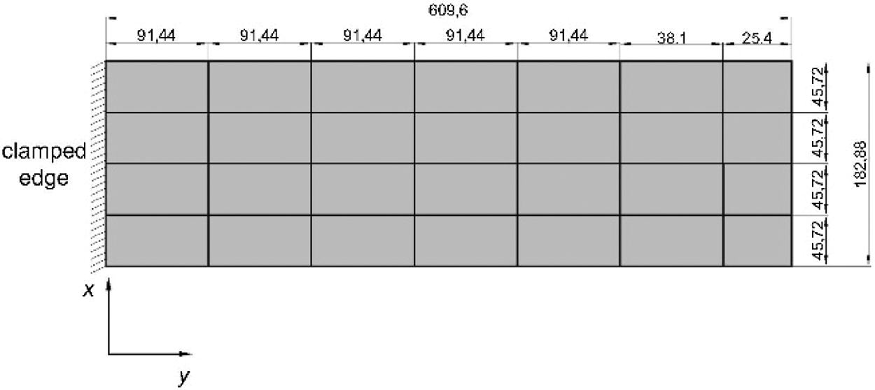
Figure 4: Discrete cantilever plate model with iDKQ4

High-fidelity FEM analysis is performed with ABAQUS, a commercially available finite element software, to generate the strain data as input of iFEM calculation. Moreover, The displacement field calculated by FEM analysis can also be used as a benchmark to examine the reconstruction accuracy of iFEM. Contour plots for the transverse displacement are compared between the iFEM and high fidelity FEM analyses as shown in Fig. 5. It can be seen that the transverse displacement field reconstructed by iFEM is basically consistent with that calculated by FEM. The percent difference between the iFEM and FEM predictions for the maximum deflection is only 0.01%; this result is slightly batter than the predictions of Tessler and Kafel.

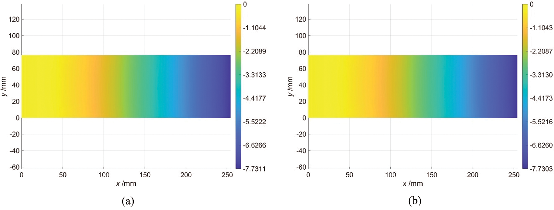
Figure 5: Transverse displacement field derived from (a) direct FEM analysis (b) iFEM analysis

3.2 A Thin-Walled Cylinder Model

In Section 2, the calculation accuracy of the iDKQ4 element is verified by a simple cantilever plate model. However, structures with complex topology are very common in practical engineering applications. Therefore, in this section, the robustness and adaptability of the iDKQ4 element in modeling complex shell structure are verified with a quarter of a thin-walled cylinder shell (as shown in Fig. 6). The diameter of the cylinder shell is 1 m, the height is 1.5 m and the uniform thickness is 3 mm. The cylinder is made of aluminium alloy having an elastic modulus of 73.084 GPa and the Poisson’s ratio of 0.33. The cylinder shell adopts the boundary condition that the lower edge is fixed, and 100N concentrated force is applied at two positions of the upper edge, respectively.

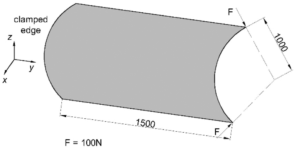
Figure 6: Schematic diagram of cylindrical shell model

The finite element convergence is studied to establish an exact reference solution of the problem. In FEM calculation, 930 rectangular S4R elements are used to discretize the cylindrical shell uniformly. In order to facilitate the transmission of strain data, iFEM calculation adopts the same discretization with FEM analysis. As shown in Fig. 7, each element has two strain rosettes, one on the centroid of the top surface and the other one on the centroid of the bottom surface resulting 1860 strain rosettes in total.

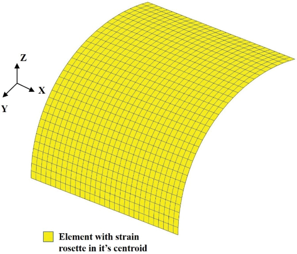
Figure 7: Discretization of cylindrical shell using 960 iDKQ4 elements with strain rosettes per each element

The displacement field calculated by direct FEM analysis and the reconstructed result by iFEM are shown in Fig. 8. It can be seen from the figure that the calculation results of FEM and iFEM are graphically indistinguishable; The reconstruction error of iFEM in Ux direction is only 0.97%; The reconstruction error of iFEM in Uy direction is only 0.98%. Although the calculation results are satisfactory, too many strain rosettes are used. Therefore, it is worthful to explore the accuracy of reconstruction of iFEM with sparse strain data (402 strain rosettes are used as shown in Fig. 9).

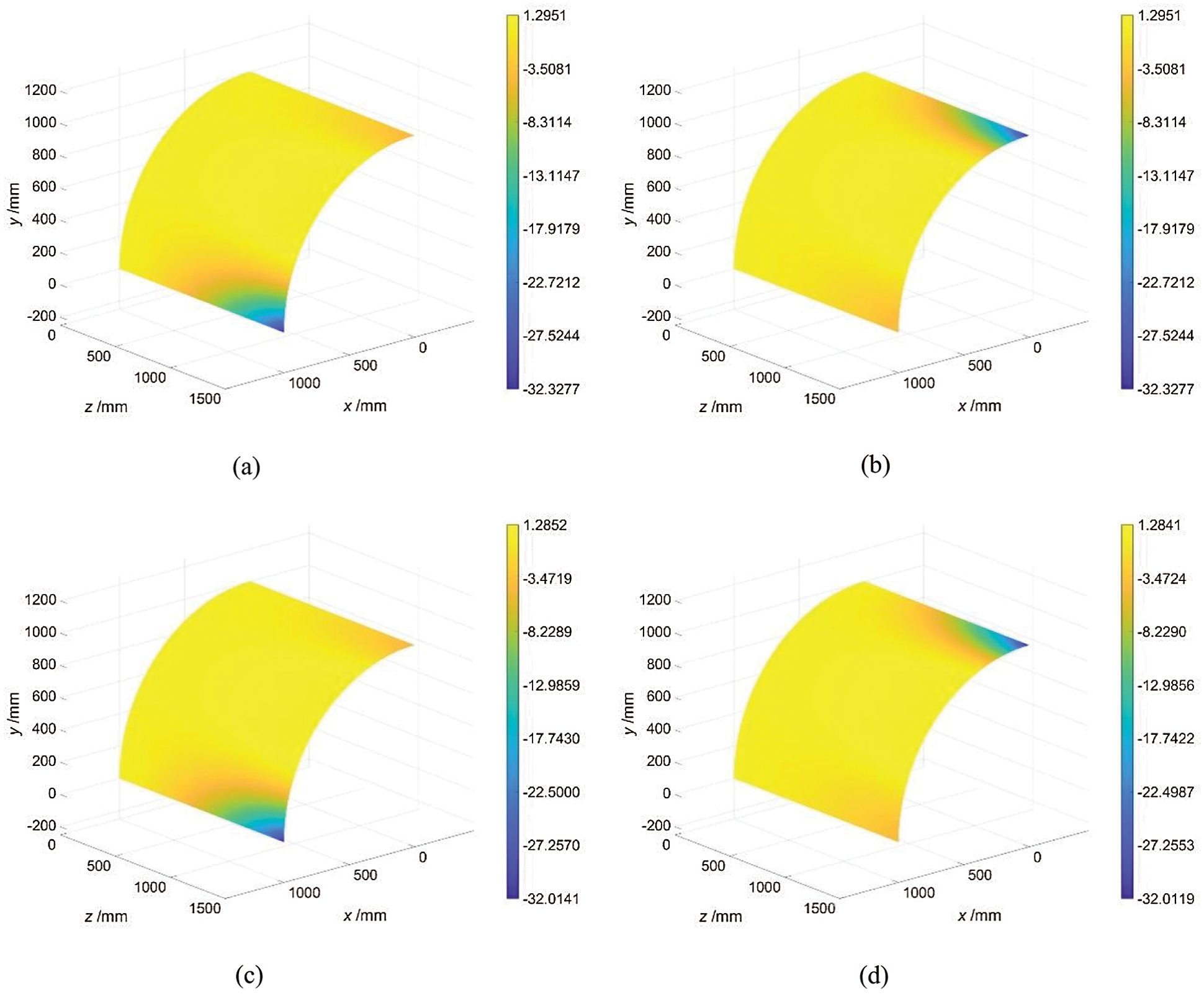
Figure 8: Displacement field in x direction calculated by (a) FEM (b) iFEM, displacement field in y direction calculated by (c) FEM (d) iFEM

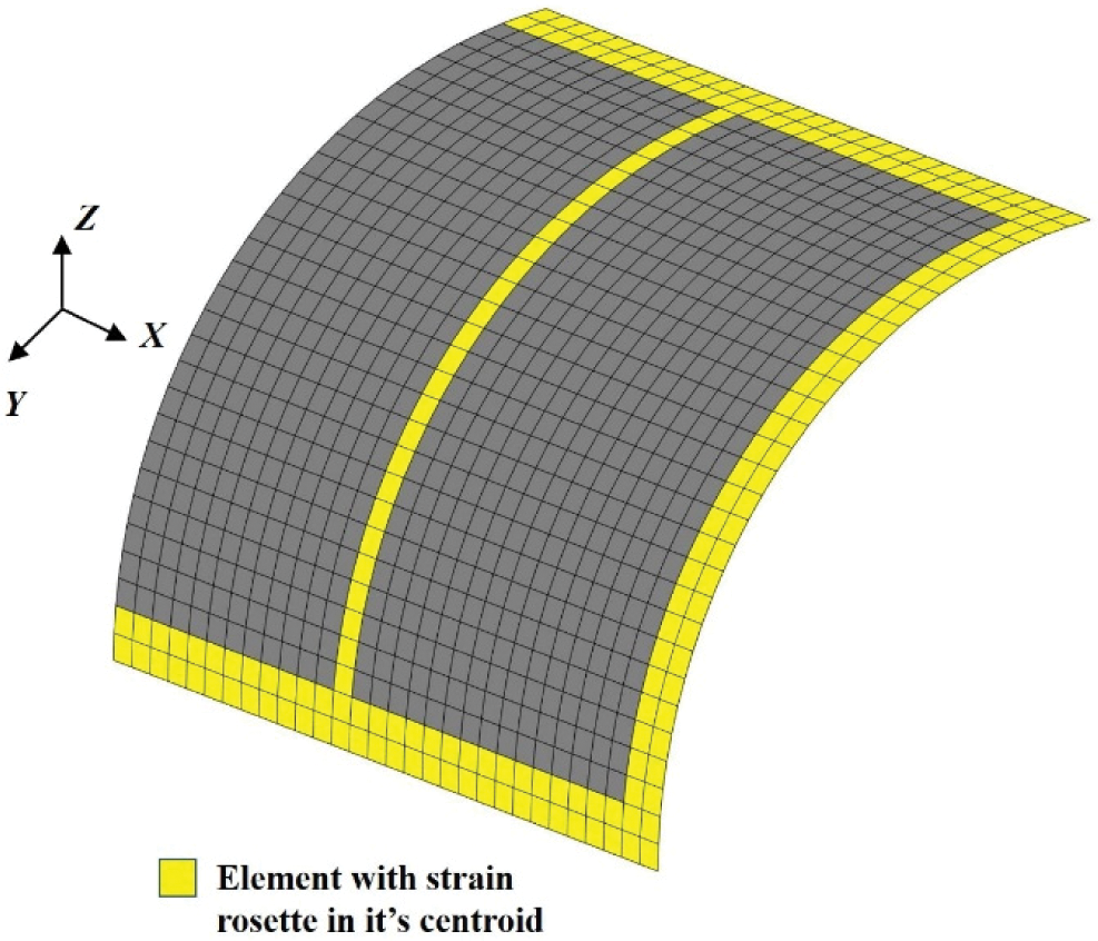
Figure 9: Discretization of cylindrical shell using 960 iDKQ4 elements with strain rosettes located within 201 select elements

In Fig. 10, the contour plots for the Ux and Uy displacement are depicted for the iFEM analyses. And the corresponding FEM analysis result is depicted in Figs. 8a and 8b. It can be seen that iFEM can accurately reconstruct the deformation tendency of the structure even with a few of strain data. The prediction error of the maximum displacement in Ux direction is 4.52%; The prediction error of the maximum displacement in Uy direction is 4.61%. The iFEM predictions remain sufficiently accurate even with sparse strain-rosette data.

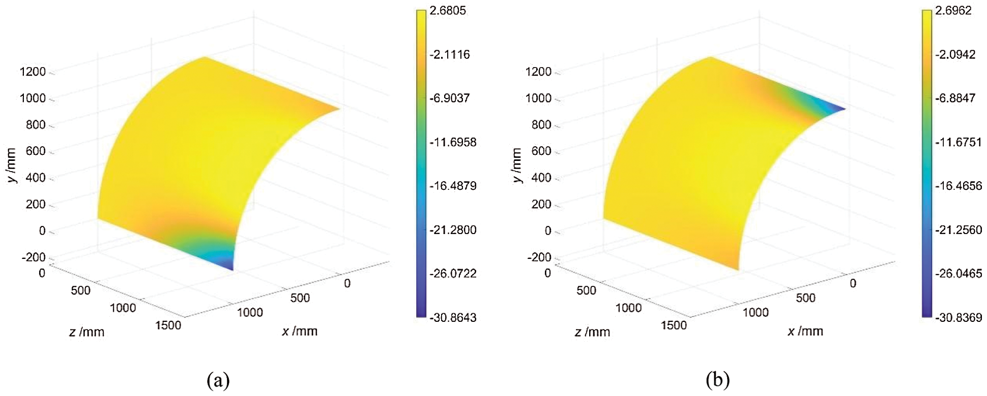
Figure 10: Displacement field in (a) Ux (b) Uy direction obtained by iFEM inversion

3.3 Shape Sensing of Composite Tank

Although having numerous advantages of high specific strength, high specific modulus, corrosion resistance and designable performance, the composite is prone to damage such as delamination and debonding, which often is invisible and has a fatal impact on the bearing capacity of the tank. The robustness and adaptability of the improved inverse finite element method/iDKQ4 element are verified by cantilever plate and cylindrical shell structures. In this section, the composite tank is investigated with the improved iFEM algorithm.

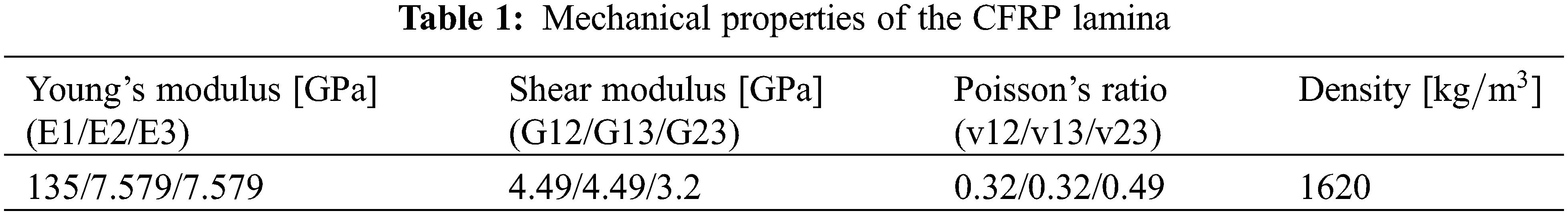
The geometric dimensions of the tank are shown in Fig. 11. The height of the straight barrel section is 458 mm and the diameter is 3338 mm; The section of the head section is an ellipse with a semi-major axis of 1669 mm and a semi-minor axis of 1043.12 mm. The radius of the upper and lower manholes is 500 mm. The reinforced composite tank adopts a symmetric stacking sequence, corresponding to [0/±45/90/±45/90/±45/0]s , with the thickness of each layer of 0.15 mm and the total thickness of 3 mm. The material properties of the single lamina are listed in Table 1.

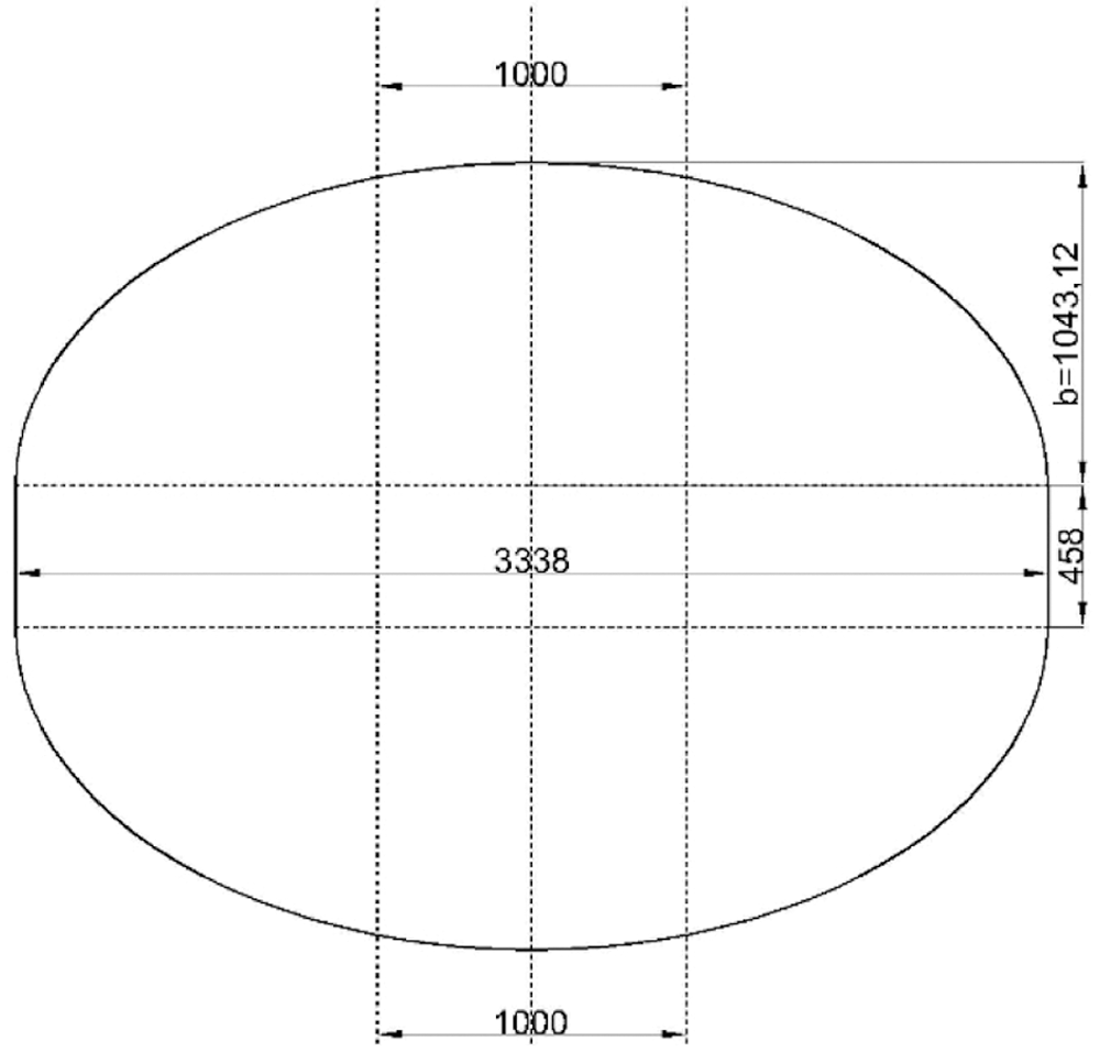
Figure 11: Schematic diagram of tank

Firstly, the linear static analysis of the tank is carried out in ABAQUS using a high fidelity grid composed of 10886 S4R shear deformation shell elements. The same grids is used for iFEM calculation and FEM analysis. The strain calculated by FEM is used as the calculation input of iFEM, and the displacement field obtained by FEM analysis is used to evaluate the prediction ability of iFEM. In order to avoid introducing errors in calculating local strain field, when the input strain field is not fully defined, elements should have a rectangular shape aligned with the input strain field direction. It is obvious that the elements of the covers do not meet this requirement, but fortunately we do not care about the results of the metal covers. In the first case study, the strain of all elements except covers can be obtain as presented in Fig. 12a. However, the number of strain rosettes used is too high to be applied to practical engineering applications. In the second case study shown in Fig. 12b, a large number of strain-rosettes are removed from elements and only the elements on 14 circumferential paths and 15 radial paths are reserved.

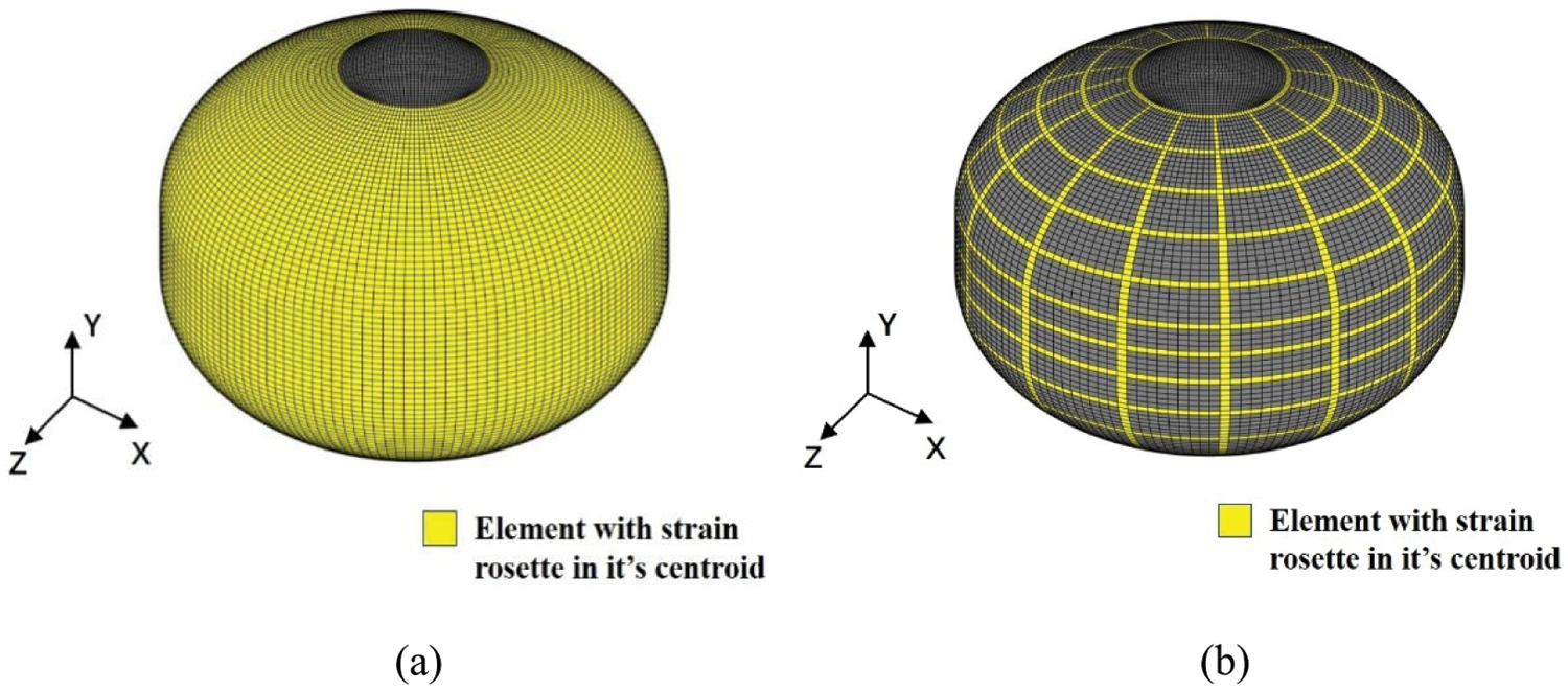
Figure 12: Discretization of tank model with strain rosettes located within (a) all elements (b) selected elements

To assess the global displacement, it is convenient to compute the axial displacement Ua and radial displacement Ur :

Ua=UYUr=Ux2+Uz2 (26)

Figs. 13a–13f presents the displacement results of FEM analysis and iFEM reconstruction. The tank expands outward uniformly under internal pressure and the result of iFEM and FEM obtains can accurately describe this trend. In Figs. 13a, 13b, 13d and 13e, the iFEM and FEM contour plots for Ua and Ur are presented, showing the results that are graphically indistinguishable. The percent difference between the iFEM and FEM solutions for the maximum values of Ua and Ur are respectively 5.85% and 1.03%. The iFEM can reconstruct the deformation of the structure relatively accurately even with sparse strain input, as shown in Figs. 13c and 13f. The percent difference between the iFEM and FEM predictions for the maximum Ur displacement is 1.80%, whereas it is only 0.38% for maximum total rotation.

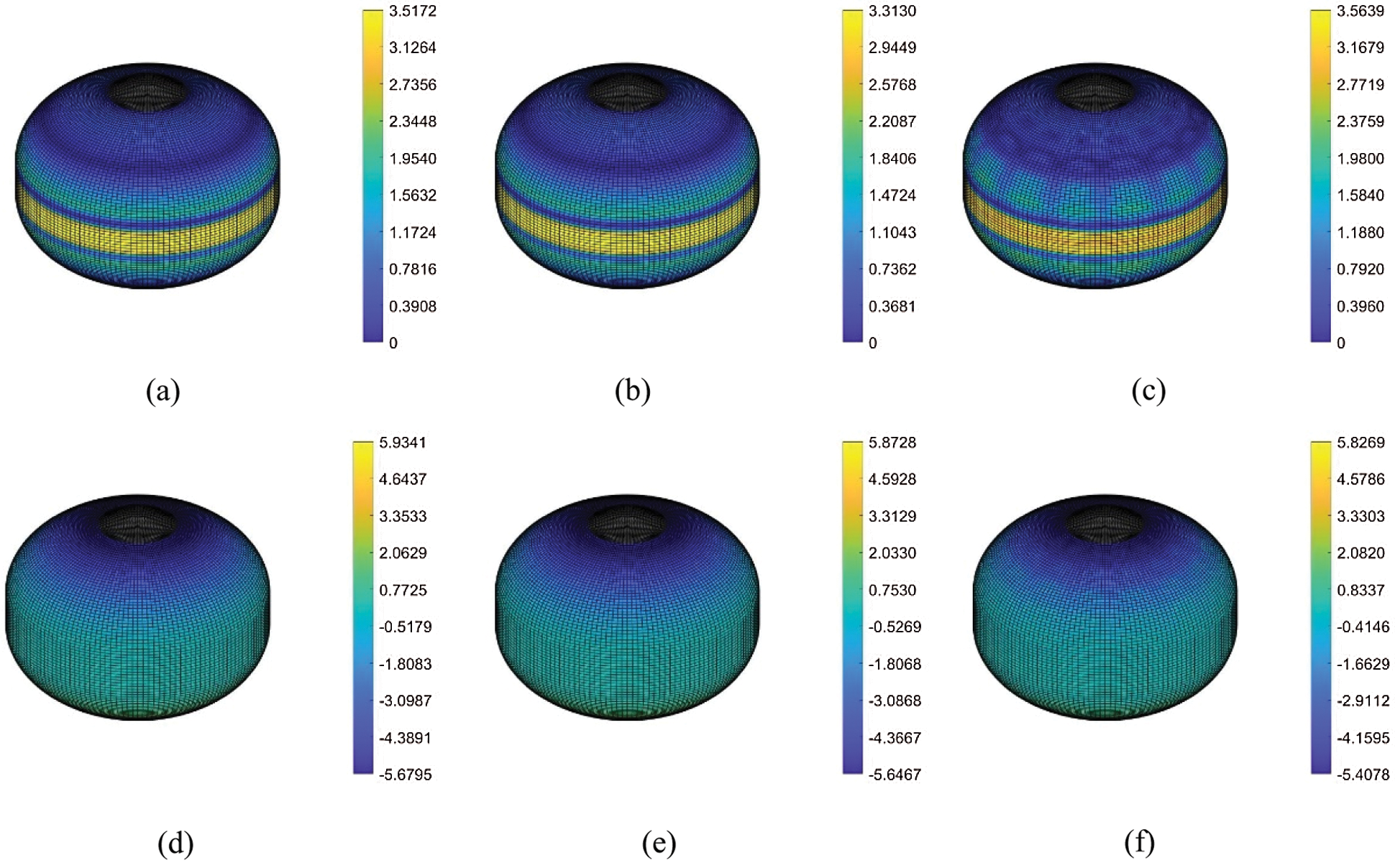
Figure 13: Displacement field in (a) Ua (d) Ur direction calculated by FEM and (b), (c) Ua (e), (f) Ur direction reconstructed by iFEM

4  Conclusion

This study proposes an improved iFEM the mathematical foundation of which is based on a least-squares functional error embracing membrane strain and curvature to solve the shape sensing problem of thin-shell structure. Subsequently, a new four-node quadrilateral inverse-shell element, named iDKQ4, is developed for numerical implementation. The robustness and adaptability of the element are verified by a cantilever plate model and a cylindrical shell model. Then, a composite tank is employed to evaluate the iFEM/iQS4 technology for application to engineering structures. Finally, the improved iFEM/iDKQ4 technology can be easily implemented and ready to applied for real-time structural health monitoring of general thin plate and shell structures.

Funding Statement: The author received funding for this study from National Key R&D Program of China (2018YFA0702800) and National Natural Science Foundation of China (11602048). This study is also supported by National Defense Fundamental Scientific Research Project (XXXX2018204BXXX).

Conflicts of Interest: The authors declare that they have no conflicts of interest to report regarding the present study.

This work is licensed under a Creative Commons Attribution 4.0 International License, which permits unrestricted use, distribution, and reproduction in any medium, provided the original work is properly cited.