Structural Durability & Health Monitoring

DOI: 10.32604/sdhm.2021.06656

ARTICLE

Influence of Unbalance on Classification Accuracy of Tyre Pressure Monitoring System Using Vibration Signals

P. S. Anoop1, Pranav Nair2 and V. Sugumaran1,*

1School of Mechanical Engineering, Vellore Institute of Technology, Chennai Campus, Chennai, 600127, India
2School of Electrical Engineering, Vellore Institute of Technology, Chennai Campus, Chennai, 600127, India
*Corresponding Author: V. Sugumaran. Email: v_sugu@yahoo.com
Received: 18 March 2019; Accepted: 07 July 2020

1  Introduction

The basic classifications for tyres are pneumatic and non-pneumatic tyres depending upon the purpose and weather. Non-pneumatic tyres, also called as airless tyres, are used in heavy vehicles at demolition sites, where the risk of tyre punctures is high. Another advantage is that airless tyres rarely go flat and hence replacement cost is less resulting in savings. The pneumatic tyres are made up of an airtight inner core which is filled with pressurized air. The pressure inside the tyre is higher than the atmospheric pressure so that the tyre remains inflated even when the weight of the vehicle is resting on it. Pneumatic tyres are highly used in automobiles. Different types of construction for tyres are radial, diagonal and bias belt models based on comfort and stability in different conditions.

In connection with the tyre indicator diagram as shown in Fig. 1, the tyre chosen for this study was coded as 165/80 R14 85 S. This type of tyre was used commonly in light motor vehicles. Here ‘165’ is the width in millimeters of the tyre cross-section, ‘80’ denotes the aspect ratio, it is the ratio of the sidewall height to the cross-section width, and ‘R’ denotes that the tyre model type is a radial tyre. ‘14’ stands for the diameter of the wheel that the tyre is designed to fit in inches. ‘85’ is the load index value. It denotes the maximum weight each tyre can carry at full speed. The corresponding value of the load index value of ‘85’ is 515 kg. The maximum safe speed for the tyre at full load is denoted by ‘S’ and it corresponds to 180 km/h. As radial tyres are commonly used for automobiles, this type was used in conducting the study as shown in Fig. 2.

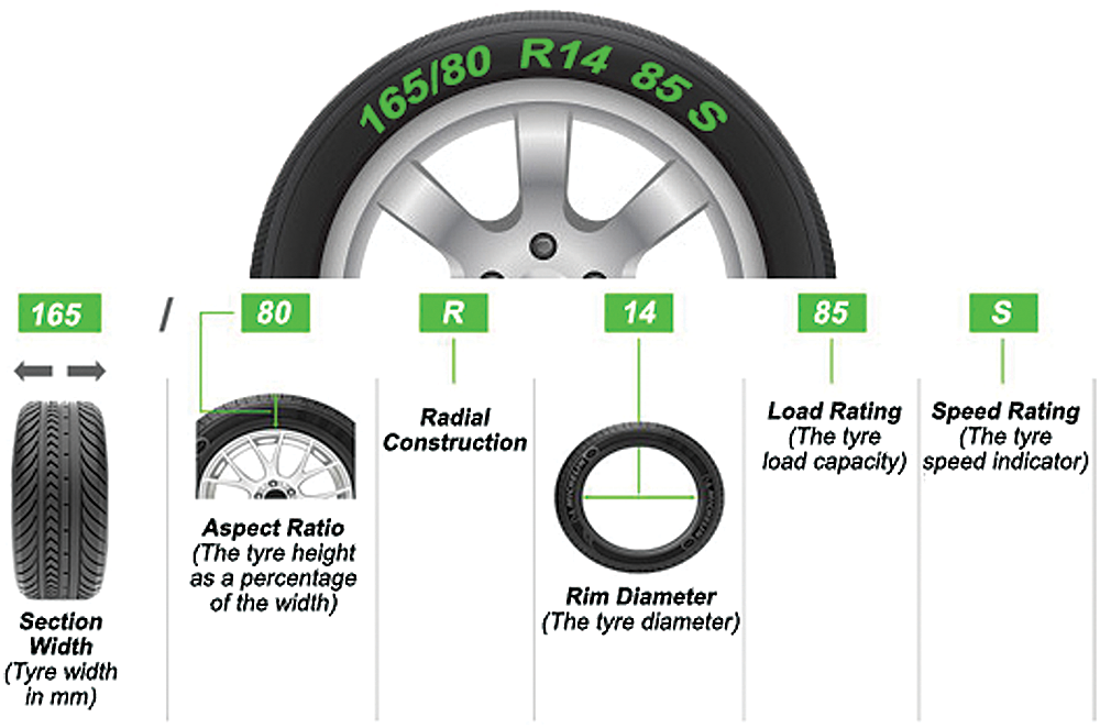
Figure 1: Tyre indicator diagram

Figure 2: Tyre used for the study

1.1 Tyre Pressure Monitoring Systems

Tyre Pressure Monitoring System (TPMS) is an assembly of several electronic subsystems including the sensors, data acquisition, and the display. These systems work together to monitor the air pressure in the tyres on a real-time basis. TPMS are classified into two categories based on the mounting of the system and affordability as Direct TPMS and Indirect TPMS.

Direct TPMS, also referred to as direct sensor type, is a system where the pressure sensors are directly mounted on the wheels or tyres of the vehicle. A pressure transducer measures the pressure inside the tyre and warns the driver in the case of over or under-inflation. Usually, for this transfer of information, RF (Radio Frequency) technology is used. In the most recent systems, the electronic assembly is made more rugged because it has to be placed inside a tyre. Micro-electromechanical systems (MEMS) are being used as sensors for pressure monitoring. The data can be transmitted to various receivers with a unique identification code. Additional information like temperature, acceleration can be recorded which makes it be an efficient tyre condition monitoring system. A TPMS warning light is installed which indicates the fault to the driver and prevents further consequences.

Indirect TPMS measures the pressure in the tyres by the rotational speed of wheels which is an indirect parameter. The initial TPMS worked on the principle that the under-inflated tyres will have a lower diameter (higher angular velocity) than the correctly inflated tyres which indicates the pressure difference and was detected. The main drawback of this system is that when all four tyres are punctured or at a lower pressure, it cannot be detected. The next generation indirect TPMS can detect the under-inflation of all the four tyres by spectrum analysis of individual tyres and can be realized by advanced signal processing techniques in software. Once the tyres are checked and all the pressures are adjusted correctly, the driver needs to reset the system using a manual button and then it is followed by a learning phase in which the system learns and stores the reference parameters. This learning phase generally takes 20 to 60 min.

The direct TPMS is expensive than its indirect counterpart. Indirect TPMS requires less programming/maintenance over the years than a direct TPMS in which resynchronization may require costly tools. In the case of indirect TPMS, overall installation hassles are less than its direct counterpart. But in the case of direct TPMS, if the battery is drained, the whole sensor must be changed and sensors are susceptible to damage during mounting/demounting. So, we have developed an Indirect TPMS by using an accelerometer module. Vibrations are used to manage the system.

Wheel balancing ensures that weight is distributed equally around the wheel and that the tyre rotates evenly. Severity of unbalance in a tyre results in vibrations of varying degrees which reverberates through the vehicle chassis. If the severity of unbalance is more, it becomes very dangerous to drive because the steering wheel experiences severe vibrations. Tyre imbalance leads to higher fuel consumption at higher speeds. An increase in wheel imbalance will result in higher levels of vibration at the fundamental wheel rotational frequency and its harmonics. Craighead proposed a method that used the vibration measurements to understand the damper condition, wheel balance and the pressure in the tyres under the normal condition of the vehicle. The accuracy of this method was 12% and it paved the way for further research to be conducted to improve the accuracy [1].

Robinson et al. proposed one of the earliest tyre pressure monitoring systems in which there was an accelerometer fixed on the tyre. Vibrations were produced by striking the tyre with a hammer and vibration signals were recorded through a signal analyzer. Variations were observed based on the change in tyre pressure [2]. Fiorletta proposed a wireless tyre pressure monitoring system which comprised of a pressure transducer, antenna and transmitter integrally housed and mounted into the tyre stem. Here, in this embodiment, the transmitter is a Surface Acoustic Wave (SAW) device that is periodically interrogated by an RF signal from the transmitter on the vehicle [3]. Mendez and Eberwine proposed a method of identification of the under-inflated or over-inflated tyres by including a microprocessor, a radio transmitter, a pressure detector and a magnetic switch for sending radio signals indicating sender ID, pressure data and change of switch state. Portable magnets were attached near the tyre and the sender ID of the wheel was detected due to the sequential transmission by the switch movements [4]. Yonetani et al. developed a tyre pressure monitoring system using the wheel speed sensors of the ABS. The monitoring system was low cost and was simultaneously able to detect the pressure loss in all the four tyres [5].

Hill et al. proposed a system that worked when the vehicle was in motion. Both methods were based on indirect TPMS in which one was a moving piston system and another one was an inductive powered transducer method [6]. Shah et al. developed a system for online detection of deflated tyres in which the vertical body acceleration signals are taken and a virtual transfer function is derived between the front and rear body acceleration signals based on certain predefined event of the vehicle. The characteristic features are generated from the frequency response of the virtual transfer function [7]. Matsuzaki et al. [8] developed a wireless system for monitoring the strain on tyres based on changes in electrical capacitance. The feature was that no sensor was used and tyre itself was used as a sensor. The sensing elements were the steel wires inside the tyres [8]. Matsuzaki et al. [9,10] developed another method where resistance and capacitance both were used as variables to measure the strain on the tyres. Li et al. [11] proposed a battery-less system for TPMS and this was done by developing a power recovery circuit. Wei et al. [12] proposed a surface-micromachining technology to integrate the piezo-resistive sensor and accelerometer for the tyre condition monitoring system.

Sham et al. [13] made an attempt to highlight the challenges in the commercialization of TPMS as a product. Ryan et al. proposed a system for safety in commercial vehicles which determines the tyre radius and pressure loss using GPS and Vehicle Stability Sensors. The algorithm is based on Kalman filter theory and operates on the assumption that there is no wheel slip, which is valid for the un-driven wheels when the vehicle is not braking [14]. Löhndorf et al. brought in the use of MEMS sensors for tyre pressure detection. The basic aim was to reduce the power consumed by the electronic system in the process [15]. Misiewicz et al. [16] proposed a pressure mapping system mainly for agricultural tyres to study the tire-soil interaction effects on the pressure in the tyres. Roveri et al. [17] developed a new technology named OPTYRE for optical strain measurements in rolling tires. The apparatus is based on the use of Fiber Bragg Gratings sensors and light spectrum analyzer. Qian et al. proposed an on-vehicle triboelectric nanogenerator (V-TENG) as a direct power source for tire pressure monitoring systems. This system was developed because the battery supply has serious limitations like environmental instability, replacement difficulty, limited durability, etc. It develops electrical energy at alarm temperature through a thermally stable polymer film [18]. Han et al. developed a model-based development approach for indirect TPMS (iTPMS). Models are categorized into three stages for model testing namely tyre model, axle model, and vehicle model. The focus was to understand the effect of tyre assembly, whole axle assembly, and the entire vehicle dynamics each individually on tyre vibration behavior [19]. Silva et al. have stated the differences between two types of indirect TPMS based on longitudinal vehicle dynamics and vertical vehicle dynamics respectively. Indirect TPMS with vertical vehicle dynamics considers the estimation of pressure based on many external parameters, unlike the longitudinal vehicle dynamics method where just the angular speeds of the wheels are considered [20]. Kang et al. developed a scheme for battery-less TPMS using the principle of wireless transmission [21]. Wu et al. developed another method based on piezoelectric materials to implement a battery-less TPMS. In this method, piezoelectric materials were used to convert the strain in tyres into electrical energy using a power recovery circuit, and this recovered power was transmitted to power the tyre data measurement unit. It has been stated that the power recovery circuit produced a stable DC voltage close to 3V and 10 mA current [22]. Yu et al. proposed a structural addition to the tyre pressure detection system. A shell was developed and the pressure detector body was placed in the housing space of the shell to make the tyre pressure detector sturdy and durable [23]. Wu et al. have studied various energy harvesting methods using TPMS and have stated that piezoelectric transducers are the most suitable method in the case of TPMS. Various factors such as installation location, suitable speed range, energy requirements, temperature, and cost have been considered to choose piezoelectric transducers [24]. Lee et al. proposed a time-varying estimation method using an Adaptive Extended Kalman Filter (AEKF) to monitor tyre stiffness. This parameter was used to assess the tyre inflation pressure using the pressure-stiffness relationship [25].

Works carried out on TPMS previously, focus mainly on sensing elements of the system and the powering unit of the system. Works have been carried out to improve the battery performance of the system to commercialize it as a product. Most of the previous works are carried out with perfectly balanced tyres. This work is focused on the wheel conditions namely balanced and unbalanced and its effects on the classification accuracy of the TPMS systems. Vibration signals were taken for the balanced condition using 40 g mass and various unbalanced condition readings for 0 g, 20 g, 60 g and 80 g in air-filled tyres. Classification accuracy and changes in trends were observed.

2  Experimental Setup

To experiment, the rear left wheel axis of the pneumatic tyre was used to obtain the vibration signals. To overcome the vibration from the engine, front-wheel drive vehicle was chosen. The two conditions that were selected for the data acquisition are balanced and unbalanced for high, normal, puncture and idle cases. Tyre pressures of 40 psi were considered high, tyre pressures of 31 psi and 19 psi were considered normal and puncture respectively. The test-driving speeds were varied from 10 km/hr to 100 km/hr. An idle state was considered irrespective of the tyre state, which was below the speed of 10 km/hr and this state did not produce sufficient amplitude of vibrations. To acquire the vibration data, a tri-axial MEMS accelerometer was used.

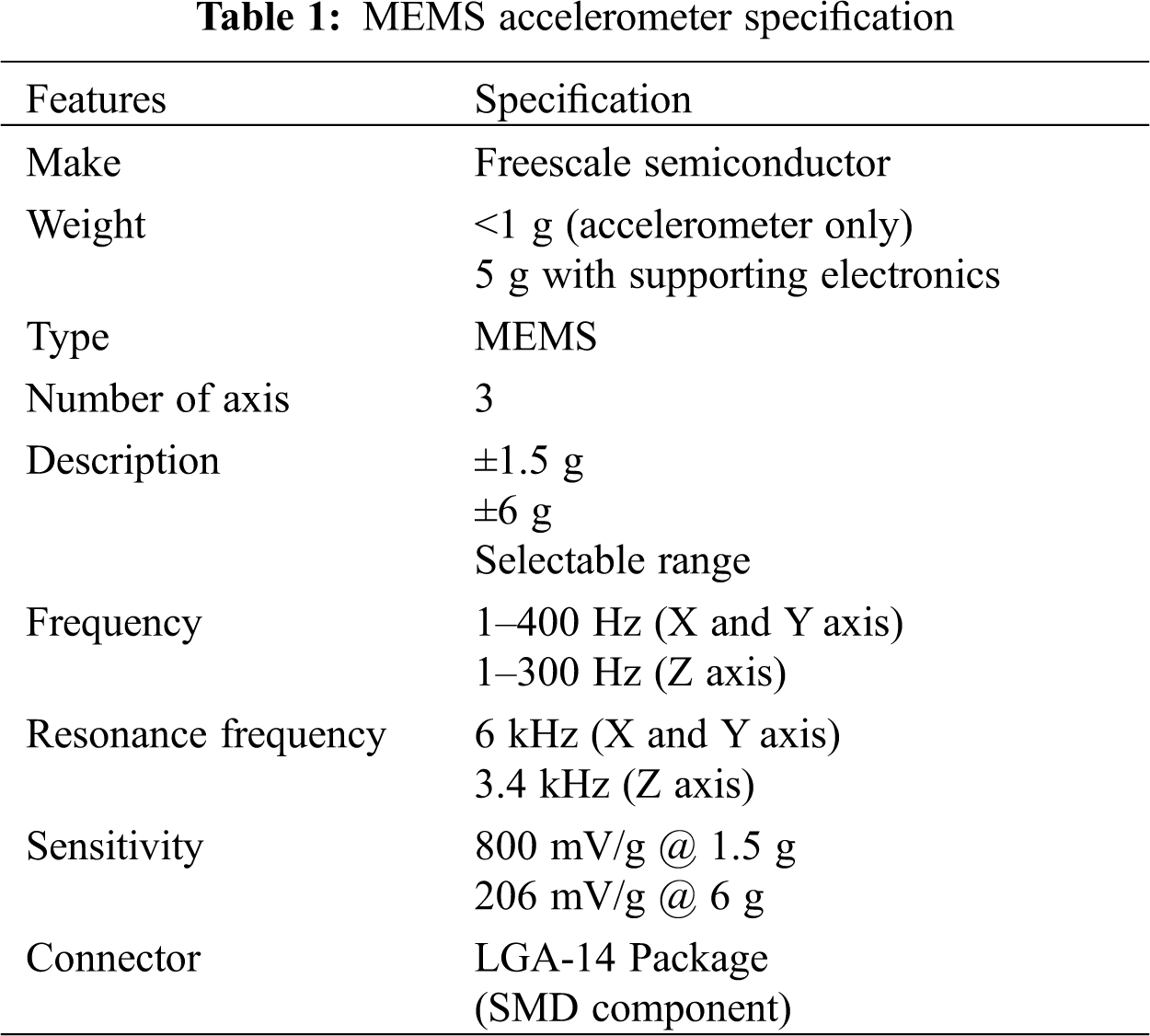
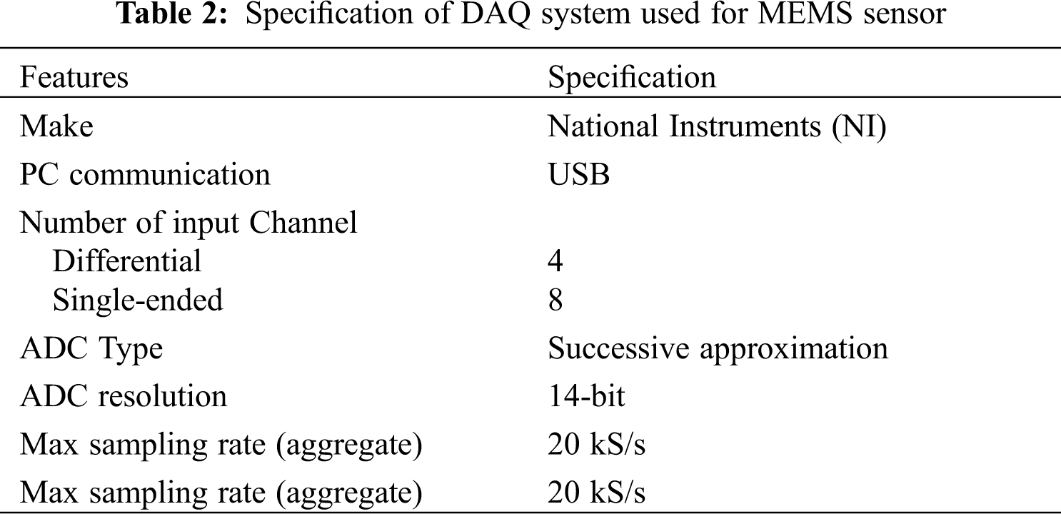
Fig. 3 explains the methodology of the work. Fig. 4 represents the MEMS accelerometer module. Fig. 5 represents the experimental setup. For the balanced and unbalanced conditions, a total of 480 samples each having a sampling rate of 1 kHz of 5000 data points were taken for both balanced and unbalanced conditions. An unbiased experiment was carried out by taking equal number of samples in all the states namely ‘High’, ‘Normal’, ‘Puncture’ and ‘Idle’. The device ‘NI USB-6001’ was used for data acquisition. A waterproof gum was coated on the accelerometer module and was fixed to the axel of the car (Fig. 4). To minimize external electronic interference, a shielded wire was used. The specifications of the MEMS accelerometer and data acquisition device were given in Tabs. 1 and 2, respectively.

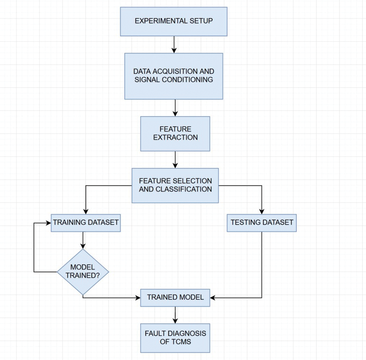
Figure 3: Methodology

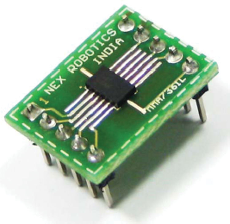
Figure 4: MEMS Accelerometer modules

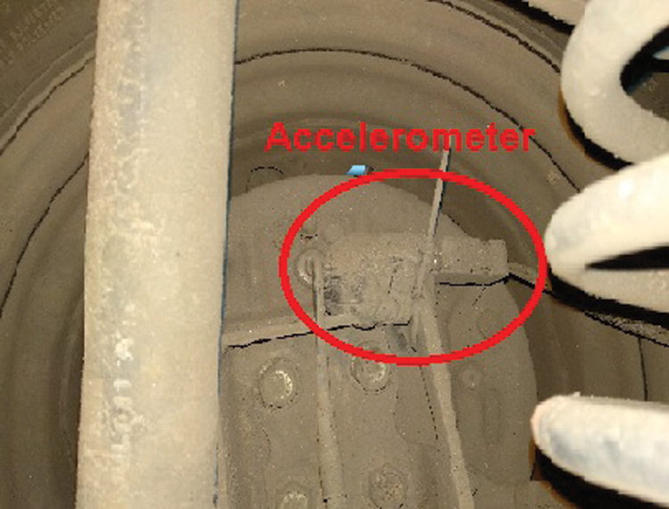
Figure 5: MEMS Accelerometer fixed on the axle

2.1 Sampling Rate Calculation

The tyre used was 165/80 radial tyre with a max pressure rating of 46 psi and the radius of the selected tyre (R) is 30.1 cm. The proposed maximum speed of the car in km/hr (S) was 100 km/hr (27.77 m/s). The minimum speed of the car in km/hr (S) is 10 km/hr (2.77 m/s). Since the wheel radius and the speed is known, RPM can be achieved by equating it to known variables (R, S). Minimum and maximum RPM & Frequency calculated by substituting the values in the following equation 2Π × (R) × f = S. From the above equation maximum frequency is 1.47 Hz and the maximum frequency is 14.73 Hz.

According to the Nyquist Shannon sampling theorem, to avoid the anti-aliasing effect, the sampling frequency should be greater than or equal to twice the maximum frequency component in the signal. Hence the minimum sampling rate must be 29.46 Hz. The sampling rate was set at 1 kHz.

3  Feature Extraction

For the good and the defective tyre conditions, the vibration signals were acquired. If these sample signals, in reference to the time as domain, are taken as inputs by a classifier, then the count of the samples should remain a constant. This number obtained is a function of the shaft speed. Therefore, this cannot be used as a direct input to the classifier. Nevertheless, some of the characteristics need to be taken out or extracted before the classification process. Descriptive statistical parameters such as sum, mean, median, mode, maximum, minimum, range, skewness, kurtosis, standard error, standard deviation, and sample variance were calculated to act as features in the feature extraction process.

•   Sum: The statistical feature value for each sample is added to obtain the sum.

•   Mean: The mathematical average of a group of values.

•   Median: The middle value separating the higher and the lower half of a data sample.

•   Mode: The value with the highest frequency in the given set of data.

•   Minimum value: Among the signals given, the lowest signal value is the minimum value.

•   Maximum value: Among the set of signals given, the highest value is the maximum value.

•   Range: The difference between the lowest and the highest signal values among a set of signals.

•   Skewness: The extent of asymmetry of a probability distribution around the mean.

Skewness=n(n−1)(n−2)∑(xi−x¯Sd)3 (1)

•   Kurtosis: It refers to the sharp nature of the peak of the distribution curve. This value is low for normal conditions and is high for the faulty condition of the blade.

Kurtosis={n(n+1)(n−1)(n−2)(n−3)∑(xi−x¯Sd)4}−3(n−1)2(n−2)(n−3) (2)

•   Standard error: Standard error is a measure of the amount of error in the prediction of y for an individual x in the regression, where x and y are the samples means and ‘n’ is the sample size.

StandardError(y)=1n−2[∑(y−y¯)2−∑[(x−x¯)(y−y¯)]2∑(x−x¯)2] (3)

•   Standard deviation: It is a measure of the deviation of the values from the arithmetic mean. In this case, it gives the power contained in a vibration signal.

StandardDeviation(σ)=n∑x2−(∑x)2n(n−1) (4)

•   Sample variance: It is the squared deviation from the mean, for any random variable in the set.

SampleVariance=n∑x2−(∑x)2n(n−1) (5)

Vibration signals were acquired for all four classes namely, High, Normal, Puncture and Idle for both balanced and unbalanced conditions. Statistical features are the most common features used to extract useful data from a signal. A total of 13 statistical features were computed. However, only a few were selected. The statistical features computed for this study were mean, median, mode, kurtosis, skewness, sample variance standard error, standard deviation, sum, minimum, maximum and range. Among them, the most contributing and prominent features were selected for the feature selection process.

4  Feature Selection

The extracted features were tested by using the decision tree. The contribution of each feature was tested and the features contributing the most were considered. The remaining features were rejected to reduce computational time and load. J48 decision tree algorithm is adapted from the C4.5 algorithm in WEKA. This algorithm is based on a tree structure and it has several numbers of branches, one root, several numbers of nodes and leaves. An attribute is associated with each node and a chain of nodes from root to leaves can be associated with the term branch. The importance of an associated attribute in a tree is provided when the occurrence of an attribute happens. Decision trees are graph-based interpretation showing every possible outcome of a decision. The J48 decision tree is one of the widely used algorithms to construct decision trees. The procedure of decision tree formation and using the same for feature selection are mentioned below:

1. The input to an algorithm is a set of features and output is the decision tree generated.

2. The decision tree has leaf nodes, which represent class labels, and other nodes associated with the classes being classified.

3. The original value or the possible values of the feature node are branches of a tree.

4. Classification of features from root to leaf node is carried out. A node provides the classification of an instance.

5. At each decision node in the decision tree, one can select the best feature for classification using appropriate estimation criteria. Concepts of entropy reduction and information gain are used to identify the best features.

Information gain basically, about how a given attribute can separate the training samples according to the target classification. As the tree grows, candidate features can be selected. Once the samples get streamlined according to the features, there will be a reduction in entropy which is measured and called information gain.

Information Gain (S, A) of a feature A relative to a collection of examples S, is defined as

Gain(S,A)=Entropy(S)−∑v∈Value(A)×|Sv||S|Entropy(Sv) (6)

where, Value (A) is the set of all possible values for attribute A, and Sv is the subset of S for which feature A has value v. Here, one can observe that Entropy (S) is the first term in the equation of Gain (S, A) from which the value is reduced as features increase. Gain (S, A) gives the entropy value which comes after the reduction by knowing a feature A. Entropy is a measure of homogeneity of the set of examples and it is given by

Entropy(S)=∑i=1c−Pilog2Pi (7)

where, c is the number of classes, Pi is the proportion of S belonging to class, i’.

The J48 decision tree algorithm has been applied to the problem for feature selection. Significance or contribution of features is an important factor and in the J48 decision tree algorithm, descending order of significance is followed by the nodes of the tree. One can see that highly contributing features appear in the tree in the top and low contributing features are in lower position of tree or ignored. One uses the concept of significance and contribution to filter out the best features. The basic idea of the algorithm is to identify the best features to classify the given data set and reduce the effort required to select features in a pattern classification case. Referring to Fig. 6, one can identify the significant features to represent the tyre conditioning monitoring systems are the standard error, sample variance, median, maximum and minimum.

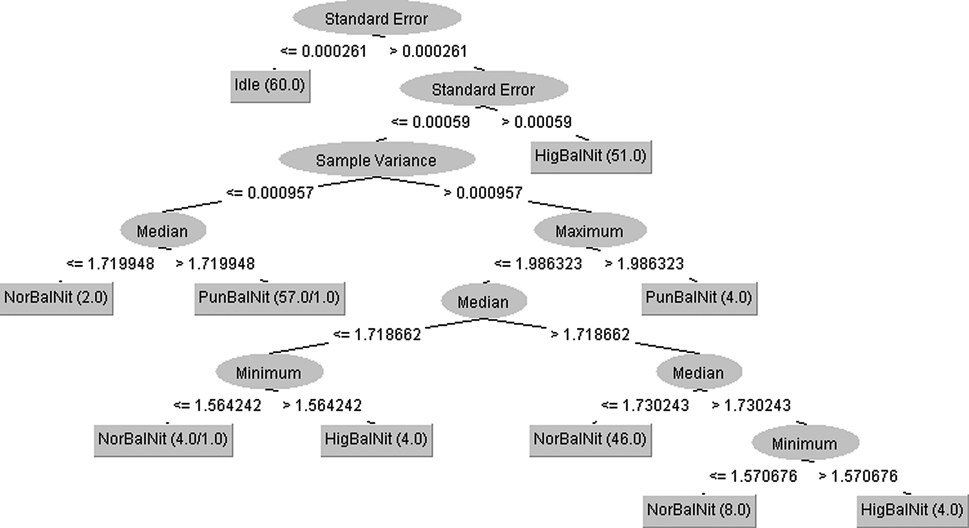
Figure 6: The generated decision tree for balanced condition using J48 algorithm

5  Feature Classification

Classification accuracy and execution time are the two important parameters in the selection of classification algorithms. Classifiers can be used to learn a mapping function from sample features to sample labels. Here, once feature selection is done, five different classifiers are used to classify the selected features. The tested classifiers are random committee, random tree, random forest, J48 and Logistic Model Tree (LMT). Random committee classifier shows the maximum accuracy level in many conditions.

5.1 Random Committee Classifier

“Random tree-based committee learning”, also called the “Random committee” is a classification method in which multiple base classifiers are selected and trained using the instances provided. The base classifier can be any classifier that forms a committee or a set to classify the instances. Here, the base classifier is a random tree and a committee or a set of random trees are formed and are iteratively trained for the instances (Fig. 7). Under default settings, Meta-random committee classification gives a classification accuracy of 81.3%.

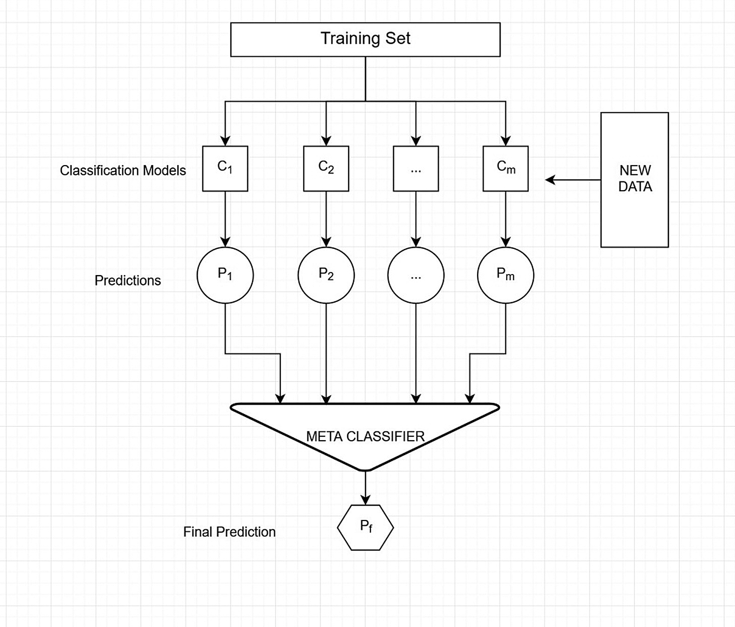
Figure 7: Ensemble learning algorithm

Random committee is a set or a class where many randomizable classifiers are brought together to build an ensemble (Fig. 8). A seed is a state of initialization of a pseudo-random number generator and here, each base classifier is built on a different seed value. To predict, the average value of all the base classifier is calculated [19].

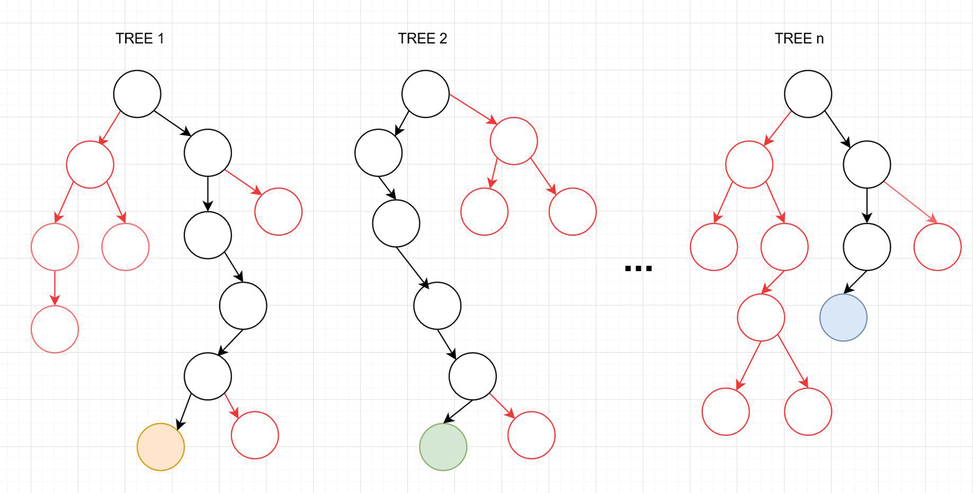
Figure 8: Random tree

6  Results and Discussions

In this work, the effects of balanced and unbalanced conditions on tyre pressure monitoring systems in air-filled tyres are evaluated. In the present experimental study, wheels are balanced by adding a mass of 40 g and readings (vibration signals) were taken. Later at 0 g, readings were taken for unbalanced conditions. There is a significant difference in the vibration signals obtained in both of these conditions. This was the fundamental motivation for studying the effect of unbalance on performance of tyre pressure monitoring systems. To do this, keeping balanced condition (40 g) as reference, weights were added in two steps and the corresponding effect on classification accuracy was noted down. Similarly, from balanced condition, weights were reduced in two steps and the corresponding effect on classification accuracy was noted down. The comparative study is presented in this section with five different classifiers.

6.1 Classification Performance for Balanced Condition

The vehicle with good tyre and balanced wheel was driven on natural style (speed varied from 10 km/hr to 100 km/hr). The tyre under study was inflated to rated pressure, called good condition, and vibration signals were taken. Similarly, puncture, high pressure, low pressure conditions were simulated on the tyre under study and the corresponding vibration signals were taken. From the vibration signals, statistical features were extracted. This forms the data set for balanced condition. With this data set, classifications were performed with five different classifiers and the classification accuracies are plotted in Fig. 9.

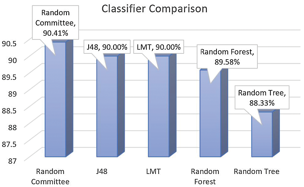
Figure 9: Classification accuracy of different classifiers for balanced condition

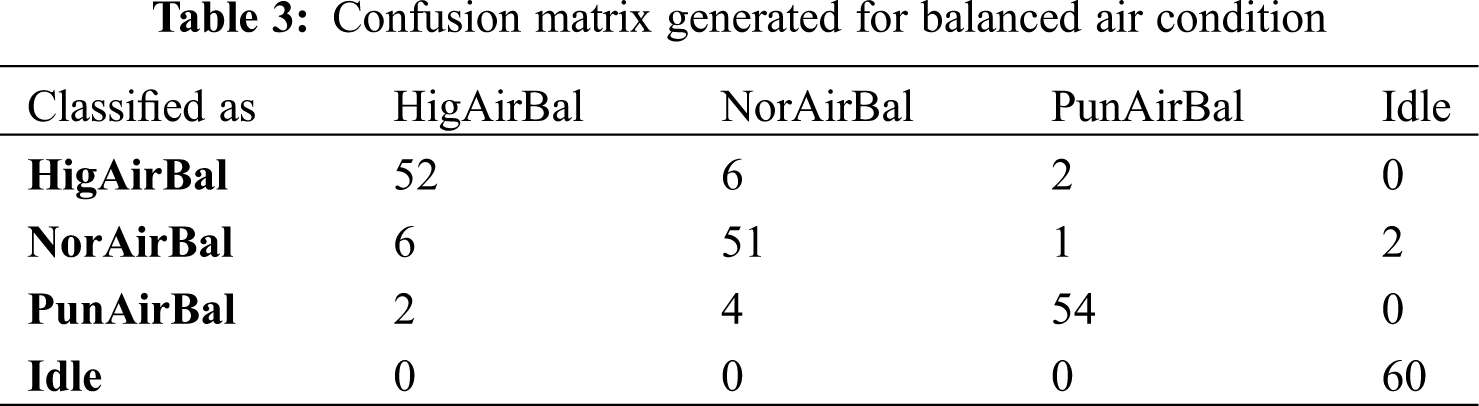
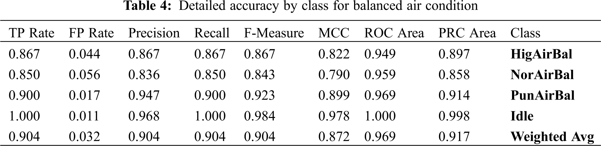
From Fig. 9, it is evident that the random committee classifier has the highest accuracy as compared to the rest of the classifiers. Random committee classifier provides the maximum classification accuracy of 90.41% for balanced air condition. The confusion matrix for balanced air condition generated by trained random committee classifier is shown in Tab. 3. Tab. 4 shows class-wise detailed accuracy for the trained random committee classifier for balanced air condition.

To fine tune the classifier, the number of iterations and the seed value are the two important parameters considered for a random committee classifier. For balanced conditions, the classification accuracy of the algorithm is plotted with the seed value and the number of iterations in Figs. 10 and 11, respectively.

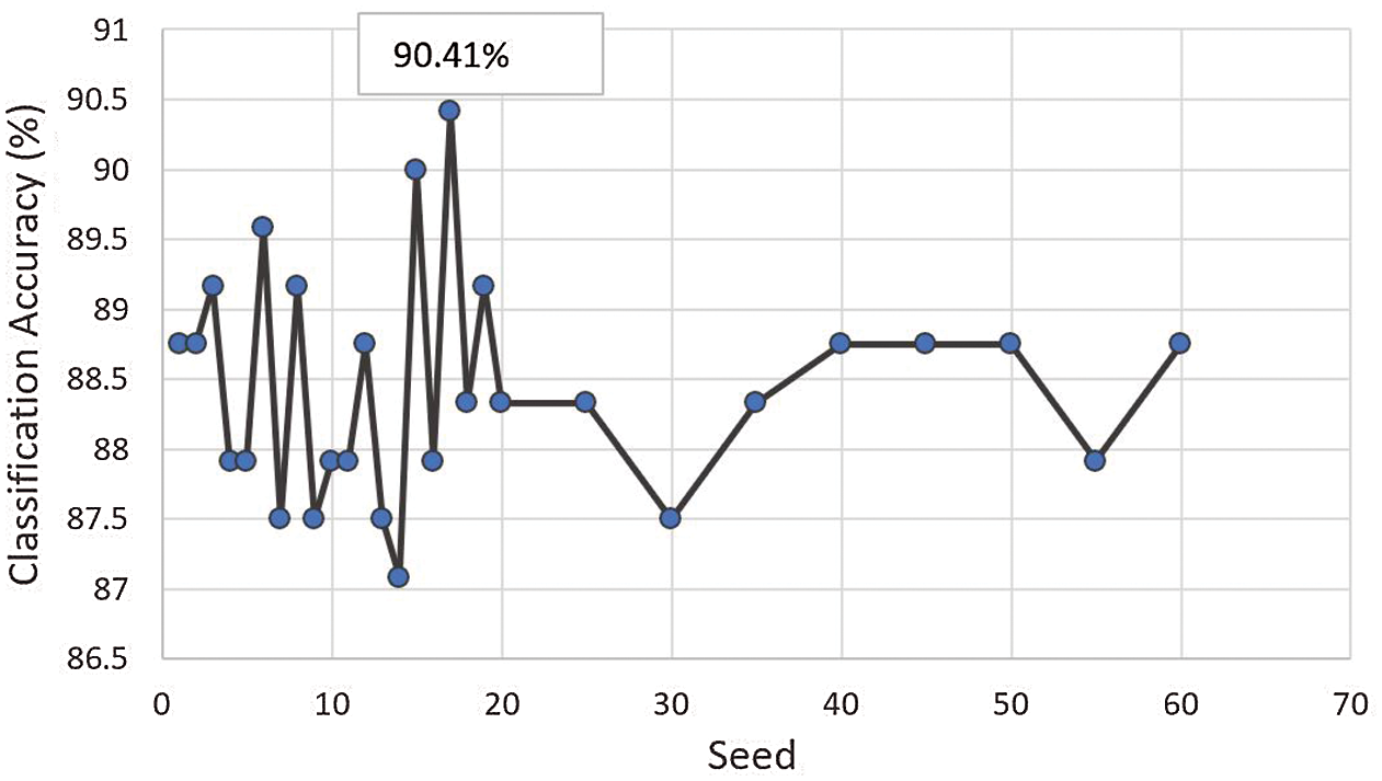
Figure 10: Seed value vs. the classification accuracy for balanced condition

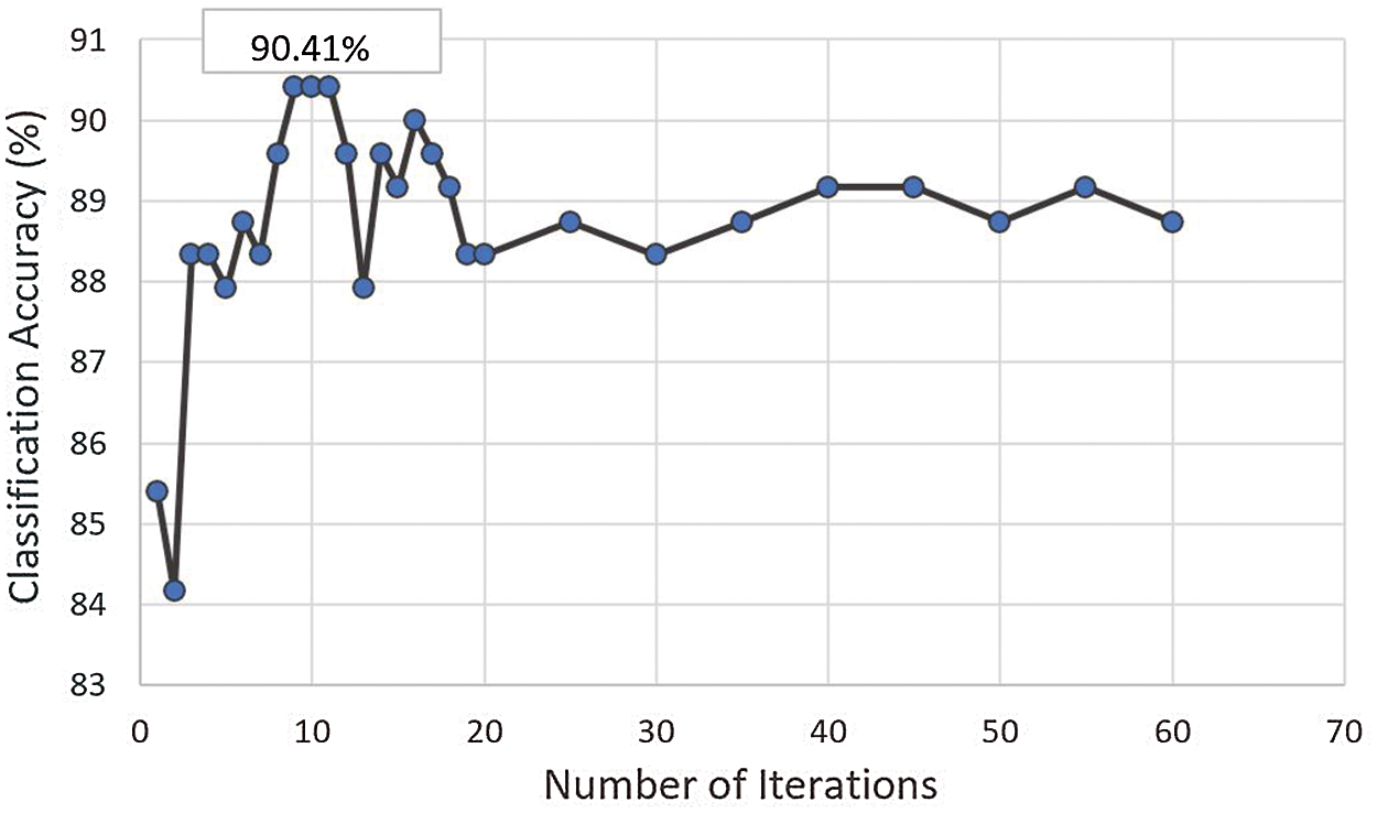
Figure 11: Number of iterations vs. the classification accuracy for balanced condition

From Figs. 10 and 11, one can find that the classification accuracy of the random committee classifier using the balanced air condition is 90.41%. The correctly classified instances (out of 60) are represented as diagonal elements in the confusion matrix. The confusion matrix for the balanced condition is shown in Tab. 3. From the table, one can notice that 60/60 of ‘idle’ instances were correctly classified followed by ‘puncture’ instances where 54/60 are correctly classified. 52/60 instances are correctly classified for ‘high’ state and 51/60 instances for ‘normal’ state.

For the random committee classifier underbalanced condition, kappa statistics was measured to be 0.8722. It measures the arrangement of likelihood with the true class. The mean absolute error is used to measure the closeness of the prediction to the ultimate result which was measured to be 0.0706. The root mean square error value was measured to be 0.2046.

6.2 Classification Performance for Unbalanced Condition

The vehicle with good tyre and unbalanced wheel was driven on natural style (speed varied from 10 km/hr to 100 km/hr). The tyre under study was inflated to rated pressure, called good condition, and vibration signals were taken. Similarly, puncture, high pressure, low pressure conditions were simulated on the tyre under study and the corresponding vibration signals were taken. From the vibration signals, statistical features were extracted. This forms the data set for balanced condition. With this data set, classifications were performed with five different classifiers and the classification accuracies are plotted in Fig. 12.

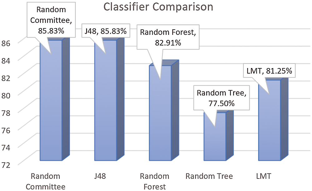
Figure 12: Classification accuracy of different Classifiers for unbalanced condition

From Fig. 12, it is evident that the random committee classifier has the highest accuracy as compared to the rest of the classifiers. Random committee classifier provides the maximum classification accuracy of 85.83% for unbalanced air condition which has reduced as compared to the balanced condition.

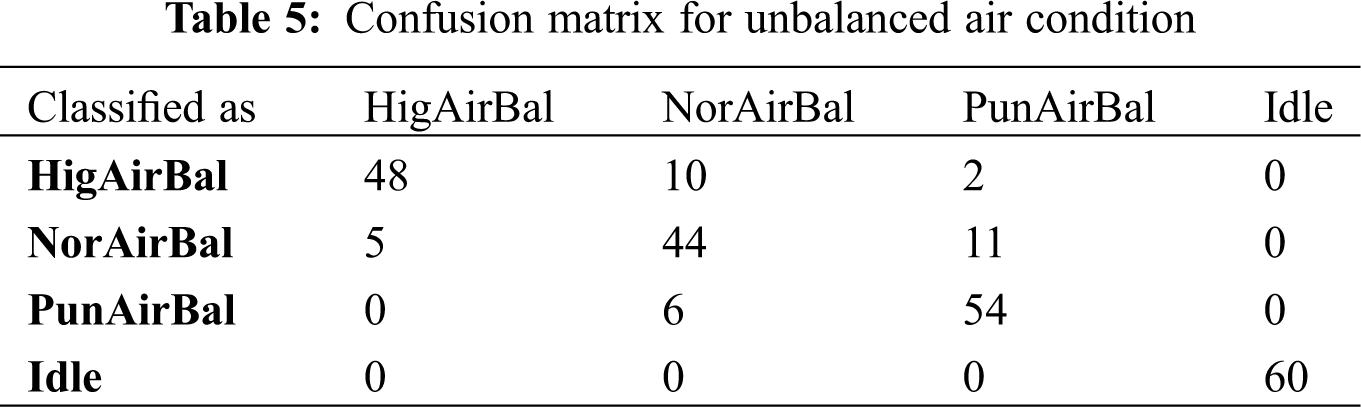
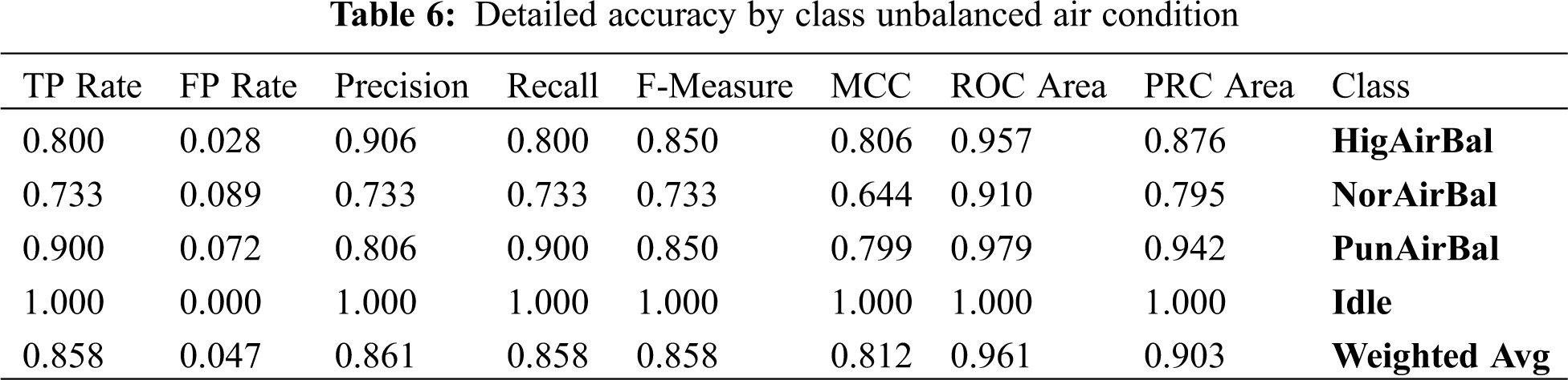
The confusion matrix for unbalanced air condition generated by trained random committee classifier is shown in Tab. 5. Tab. 6 shows class-wise detailed accuracy for the trained random committee classifier for unbalanced air condition.

The random committee classifier depends on two variables namely seed value and number of iterations. The variation of these parameters vs. the algorithms classification accuracy for the unbalanced condition is plotted in Figs. 13 and 14, respectively.

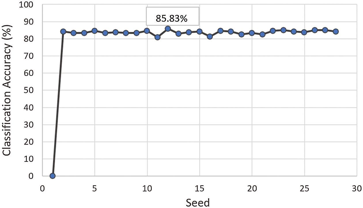
Figure 13: Seed value vs. the classification accuracy for unbalanced condition

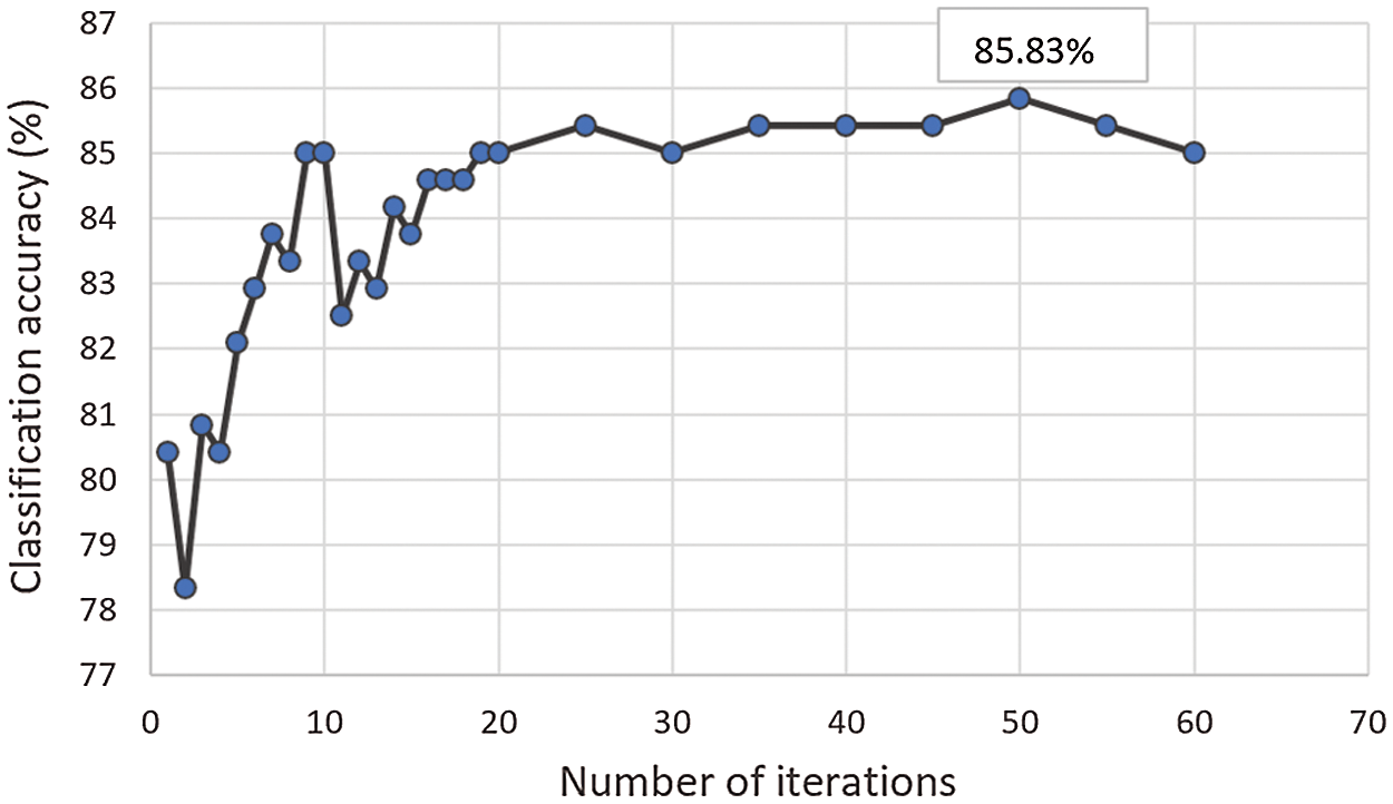
Figure 14: Number of iterations vs. the classification accuracy for unbalanced condition

From Figs. 13 and 14, one can find that the classification accuracy of the random committee classifier using an unbalanced air condition is 85.83%. The correctly classified instances (out of 60) are represented as diagonal elements in the confusion matrix. The confusion matrix for the unbalanced condition is shown in Tab. 5. From the table, we can notice that 60/60 of ‘idle’ instances were correctly classified followed by ‘puncture’ instances where 54/60 are correctly classified. 48/60 instances are correctly classified for ‘high’ state and 44/60 instances for ‘normal’ state.

For the random committee classifier under unbalanced conditions, kappa statistics was measured to be 0.8111. It measures the arrangement of likelihood with the true class. The mean absolute error is used to measure the closeness of the prediction to the ultimate result which was measured to be 0.0984. The root means square error value was measured to be 0.2343.

6.3 Trend Analysis

In the present study, when 40 g is added to the wheel, it is balanced and this will serve as reference. The curiosity is to know what happens to the performance of the TPMS when the weight increases from reference value (balanced condition) as well as when weight decreases from reference value. To study this effect, a trend analysis is performed and the results are presented here.

From Figs. 15–20, one can deduce the trends of change in classification accuracy as the unbalance in wheels is changed by adding mass. For this setup, the lowest classification accuracy is obtained when no mass is added (0 g) which is 85.83%. The highest classification accuracy is obtained at the balanced condition (40 g mass) which is 90.41%.

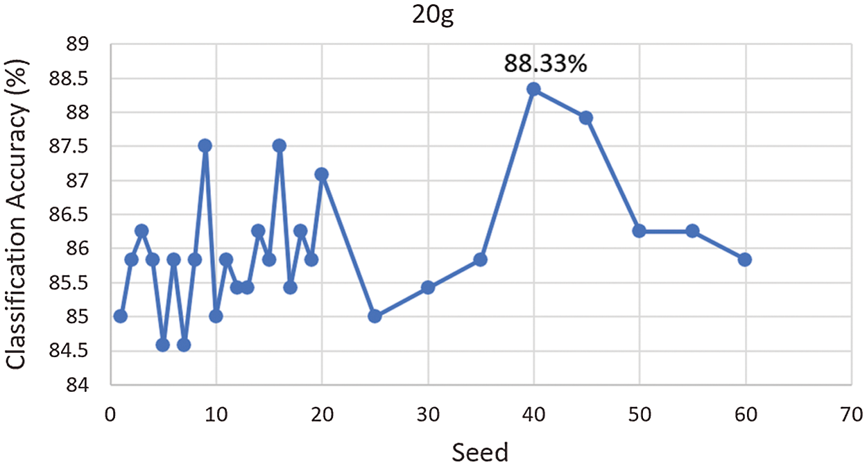
Figure 15: Seed value vs. the classification accuracy for unbalanced condition (20 g mass)

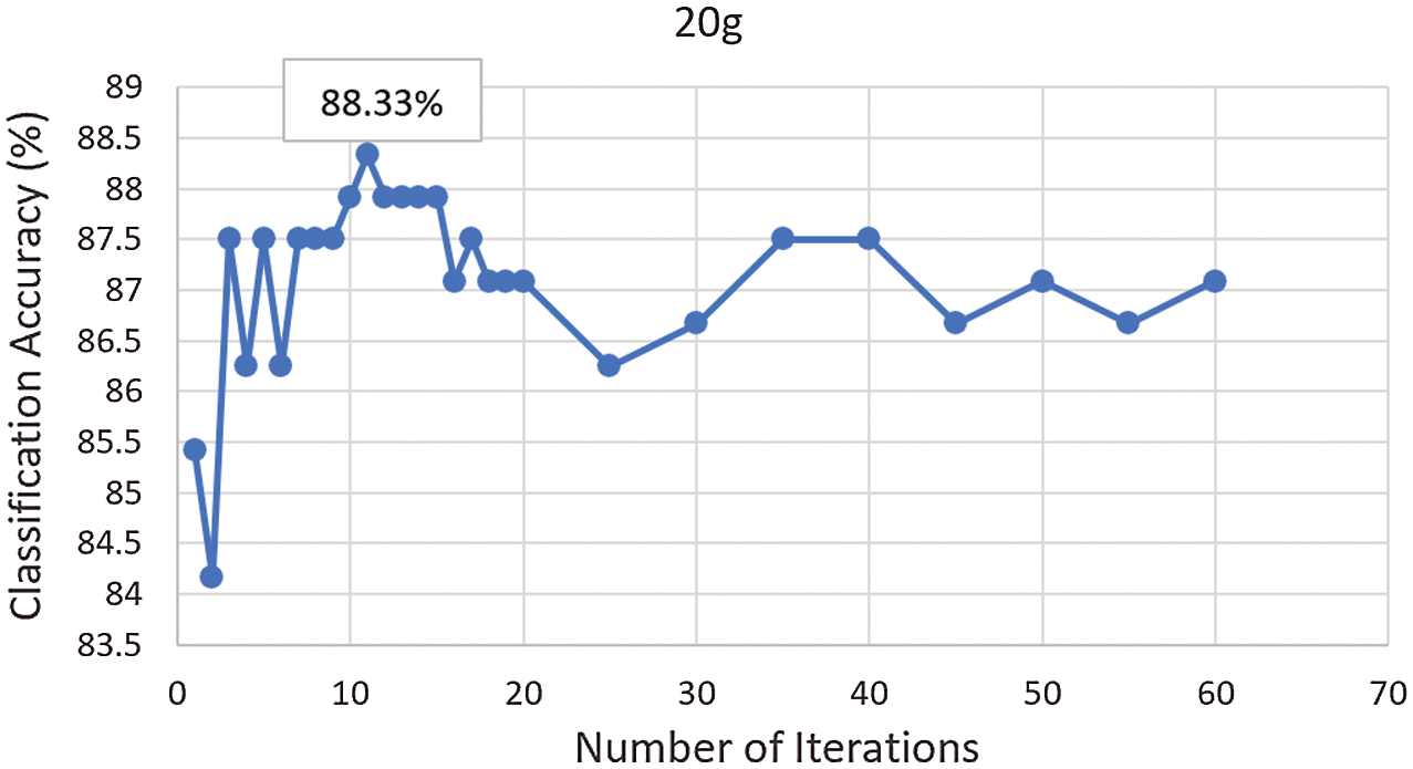
Figure 16: Number of iterations vs. the classification accuracy for unbalanced condition (20 g mass)

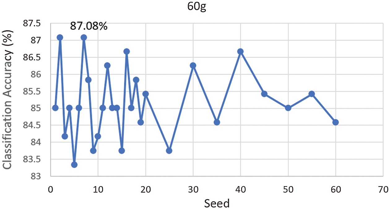
Figure 17: Seed value vs. the classification accuracy for unbalanced condition (60 g mass)

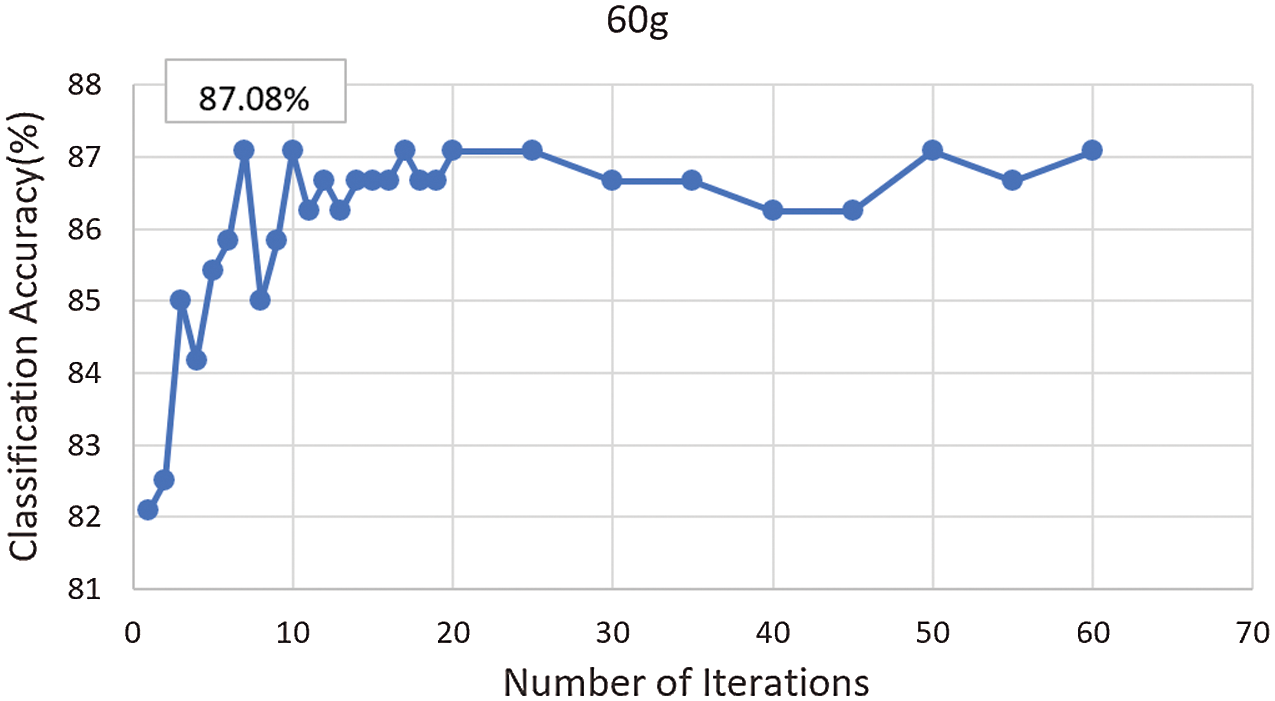
Figure 18: Number of iterations vs. the classification accuracy for unbalanced condition (60 g mass)

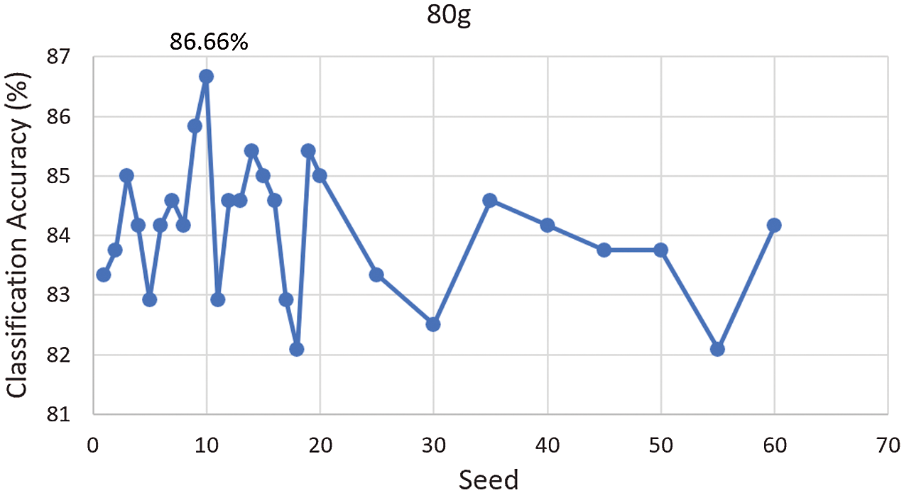
Figure 19: Seed value vs. the classification accuracy for unbalanced condition (80 g mass)

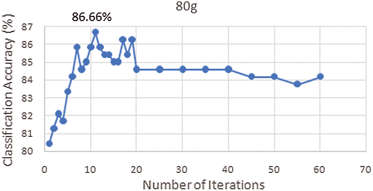
Figure 20: Number of iterations vs. the classification accuracy for unbalanced condition (80 g mass)

From 0 g, as one keeps adding mass, the classification accuracy increases till it approaches the balanced condition at 40 g. And after 40 g, one can see a significant reduction in the classification accuracy. At 20 g, classification accuracy is 88.33% which then reduces drastically to 87.08% and then reduces down to 86.66% at 80 g.

As the mass is increased above or below the balanced condition, there is a significant reduction in classification accuracy.

The balanced condition is obtained by adding 40 g mass to both the wheels. From Fig. 21, an unbalanced condition graph has been plotted, which shows the effect on classification accuracy when the wheels are unbalanced at 0 g, 20 g, 60 g, and 80 g.

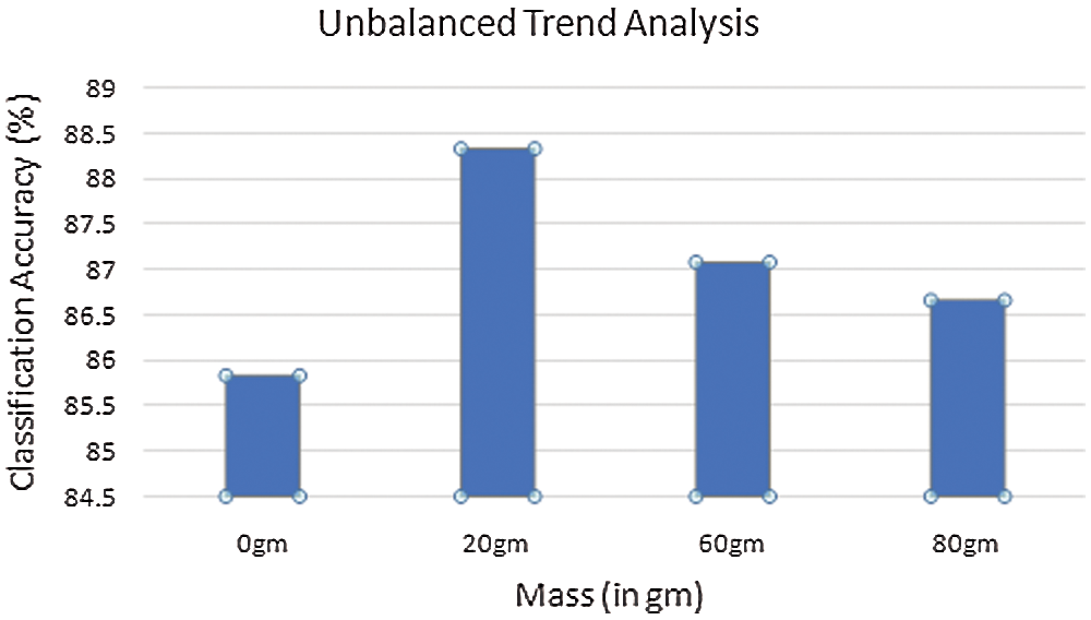
Figure 21: Unbalanced trend analysis

7  Conclusion

In the present automobile industry, tyre pressure monitoring systems (TPMS) has become an integral part because safety aspects of the vehicle are being considered as a high priority. This paper displayed a comparison of algorithm-based classification of vibration signals for the condition monitoring of tyre pressure monitoring systems. Data modelling techniques were used to create two models for each condition based on the vibration signals acquired. 10-fold validation method was used to validate the models and classification accuracy of 90.41% was obtained for random committee classifier using balanced air condition and the lowest classification accuracy was 85.83% for random committee classifier using the unbalanced air condition for this setup. From the balanced condition at 40 g, an unbalance is created by reducing or increasing mass, classification accuracy reduced. The error rate is relatively less and may be considered for tyre condition monitoring. In future, one can reduce the mass spacing to 5 g and perfectly find the balanced condition which gives us the maximum classification accuracy and also monitor the minute changes in classification accuracy.

Funding Statement: The authors received no specific funding for this study.

Conflicts of Interest: The authors declare that they have no conflicts of interest to report regarding the present study.

This work is licensed under a Creative Commons Attribution 4.0 International License, which permits unrestricted use, distribution, and reproduction in any medium, provided the original work is properly cited.