Structural Durability & Health Monitoring

DOI: 10.32604/sdhm.2021.014256

ARTICLE

Inverse Load Identification in Stiffened Plate Structure Based on in situ Strain Measurement

Yihua Wang1, Zhenhuan Zhou1, Hao Xu1,*, Shuai Li2 and Zhanjun Wu1

1Faculty of Vehicle Engineering and Mechanics, Dalian University of Technology, Dalian, 116024, China
2Nantong Ocean and Coastal Engineering Research Institute, Hohai University, Nantong, 226000, China
*Corresponding Author: Hao Xu. Email: xuhao@dlut.edu.cn
Received: 14 September 2020; Accepted: 25 December 2020

1  Introduction

With increasing demands for high-performance engineering structures, structural health monitoring (SHM) has received widespread attention, where the importance of load identification, as a major SHM task, has been widely recognized. Specifically, external load information in engineering structures is important for the estimation of structural reliability, service life, etc. [1–3]. In the scope of science and technology, many practical engineering problems are finally solved through mathematical modeling methods and establishing related differential equations that describe physical processes. Generally speaking, when we consider a structural system, the positive question we are studying is how to describe the state and physical process of the system. In fact, it is to establish a differential equation model according to some main conditions of the state and process, such as boundary conditions or initial conditions. The conditions are solved, so that a mathematical description of the physical process and state of the system can be obtained. The inverse problem of the system structure is often to determine the unknown quantity in the definite solution test by studying some known quantities or some additional conditions in the definite solution conditions given by the differential equation.

In actual engineering, there are many types of loads. Generally speaking, the method of determining the load acting on the structure is often to adopt a direct measurement method and an indirect identification method. The former is to determine the structural load through the measurement method or determine the size of the load by measuring the parameters related to the load. However, in many cases in actual engineering, it is difficult or impossible to determine the direct measurement of the external load acting on the structure. In this case, it is often only possible to determine the load by using relevant information such as the response of the structural system measured in practice, for example, from the displacement response, velocity response, acceleration response and strain response of the structure to obtain load information [4–6]. It should be noted that in the process of load identification, the identification matrix is often unclear, and measurement errors will almost inevitably occur in the actual response of the structure. The unsuitability problem will cause a significant amplification effect on the small errors contained in the measurement response, which will result in a significant reduction in the accuracy of load identification, and at the same time the identified load will have a serious deviation from the actual load. It should be noticed that in the process of load identification, the identification matrices are often ill-defined, and measurement errors are almost inevitable in the actual responses of the structures. The ill-posedness problem will induce significant amplification effect to small errors contained in the measured responses, resulting in largely reduced load recognition accuracy with severe deviation of the identified loads from the real ones.

In order to improve the accuracy of load identification, a number of methods have been developed. Amiri et al. [7] uses a new parametric impulse response matrix resume system model and applies it to wind load identification problem, and obtains satisfactory convergence speed and fitting properties. Based on the definition of virtual displacement, Jang et al. [8] transformed the problem of nonlinear system identification by establishing a system model representing linear relationship between virtual displacement response and impact load, and then obtained load identification results relying on iterative regularization. Thiene et al. [9] studied the impact of transfer function estimation on impact load identification results in composite panels, and constructed a load identification system model by proposing a method to obtain the transfer function, which effectively identified multi-point impact loads. Renzia et al. [10] used simplified finite element model based on polycondensation technology to establish a dynamic load identification model, and the dynamic loads are identified in a L-shaped plate structure. Wentzel [11] used weighted modal filtering method for load identification. Based on finite element models, loads on the truck cab suspension can be identified effectively. Compared with the traditional method, the weighted modal filtering method is effective to improve the accuracy of recognition results. Lee et al. [12] combined the extended Kalman filter and the intelligent regression least square method to effectively identify the external dynamic load acting on the tower structure. Cao et al. [13] used the artificial neural network method to study the dynamic load identification problem on the wing, and pointed out that the artificial neural network has a faster convergence speed and a higher load identification accuracy. Gupta et al. [14] proposed a method for establishing a system model in time domain by using measured structural strain response to identify dynamic loads, with model reduction technology was used to simplify the system model to large extent. Liu et al. [15] compared dynamic load identification methods based on truncated singular value decomposition, least squares method and total least squares method, respectively. Jian et al. [16] proposed a moving load identification method based on generalized orthogonal functions and regularization. The finite element method was used to establish the bridge vibration equation. There are generalized orthogonal functions to determine the modal response and according to the principle of mode superposition. Its derivative, using regularization techniques to get stable is the result. Han et al. [17–19] used Green impulse function or Heaysiside step function to discretize the dynamic response relationship of the system. Through the optimization method, they reversed the concentrated load and distributed load on the laminated plate, and proceeded from the principle of variational and spectrum analysis respectively. The research on the influence of regularization method and singular value decomposition method on the reverse seeking effect, and the corresponding research on the influence of the uncertainty problem on the reverse seeking result. Perotin et al. [20,21] studied the identification of distributed random loads. He proposed an orthogonal decomposition technique based on structural modal models and spatially distributed loads, and used regularization techniques to determine the orthogonality of loads. Decomposed Fourier coefficients to determine the spatially distributed random load acting on the structure, then, the vibration coefficient of the fluid load acting on the pipe structure is taken as the research object, and the proposed method is applied to reconstruct the vibration of the pipe structure caused by the fluid Load. French scholars Pezerat et al. [22,23] proposed a distributed dynamic load identification method based on modal filtering and differential form, and then extended the proposed method, using a regularization method based on singular value decomposition to identify the distributed dynamic load acting on the board. The spatially distributed load acting on the thin cylindrical shell is reconstructed by the spatial filter solution method. Zhong et al. [24] took the bridge structures commonly used in highway bridges and urban overpasses as the research object, established a bridge moving load identification model based on the grid method, deduced the spatial motion equation of the bridge under moving loads, and solved the discrete vibration mode of the bridge structure using the subspace iteration method, And finally adopt the spline approximation method and the truncated singular value decomposition regularization method to obtain the stable solution of the moving load. Trabelsi et al. [25] studied a typical problem of identifying unstable rotational force on fan blades caused by long-distance sound pressure, and using Tikhonov regularization solution method to effectively overcome the of the ill-conditioned issue of the system. Busby et al. [26] use Tikhonov regularization method in load identification, use dynamic programming theory to determine regularization parameters, and use cantilever beam model for numerical simulation. Choi et al. [27] researched and compared the GCV method, OCV method and L curve method for the identification of dynamic loads in plate structure under different noise levels. According to the results, L-curve method is most accurate in load identification under large noise levels, and the OCV method shows higher accuracy at low noise levels.

While load identification methods have been applied in practical engineering, most existing studies are focusing on the utilization of displacement response [4,7,8,10], velocity response [7,25] and acceleration response [7,11,15,27] on relatively simple structural geometry. Studies using strain responses captured on strengthened structure are still rare. In this paper, structural strain responses are used to identify different forms of loads on a strengthened plate structure, and the performances of truncated singular value method, GCV method and OCV method are compared. With demonstrated high accuracy, the GCV method is then used to identify concentrated loads in three different directions (i.e., vertical, lateral and longitudinal) exerted on a stiffened plate. The results show that the GCV is able to effectively identify multi-source static loads, with relative errors less than 5%. Moreover, under the situation of swept frequency excitation, the GCV can achieve much higher accuracy compared with direct inversion, with averaged recognition error less than 10%.

2  Transfer Path Analysis

For load identification in linear systems, it is often assumed that the load positions are known, and the magnitude and direction of the loads need to be determined. According to the concept of classic transfer path analysis (TPA), the relationship between the loads and structural responses can be expressed as follows:

{x1x2⋮xm}=[h11h12⋯h1nh21h22⋯h2n⋮⋮⋮⋮hm1hm2⋯hmn]{f1f2⋮fn} (1)

where n is the number of loads; m is the number of responses; hij is the element in the response matrix, linking the jth response to the ith load. In applications, n and m are usually not equal.

Eq. (1) can be rewritten in a general form as

X=HF (2)

where X is the measured response vector, F is the load vector to be identified, H is the response matrix. By applying equivalent and uniform loads at each load position, the response matrix can be formed based on the measured responses.

Based on direct matrix inversion, the force vector in Eq. (2) can be obtained to be

F=H+X (3)

where H+ is the generalized inverse of the response matrix H . The direct inversion method may lead to ill-conditioned problems. Therefore, the key step is to solve the ill-conditioned problems that may exist in the system. Truncated Singular Value Decomposition (TSVD) method and Tikhonov regularization method are introduced as follows.

3  Truncated Singular Value Decomposition Method

The TSVD is established based on conventional Singular Value Decomposition (SVD), and the essence of solving ill-posed problem is to modify the singular values of the response matrix H . Given the rank of the response matrix H is r (r > 0), orthogonal matrices of H , i.e., Um×m and Vn×n , can be found for the implementation of SVD, that is

Hm×n=Um×mSr×rVHn×n (4)

where Um×m=(u1,u2,⋯,um) , Vn×n=(v1,v2,…,vn) , S=diag(s1,s2,…sr) with s1≥s2≥...≥sr≥0 ; and VH is the Hermitian transpose of matrix V . It has

F=H+X=1s1u1Hv1X+1s2u2Hv2X+...+1srurHvrX (5)

where u and v are the vectors in U and V . The TSVD method is to discard k smaller singular values in the response matrix H . If the discarded singular values are much smaller in magnitudes than the other singular values, only a small portion of the information of the matrix H will be lost. At the cost of sacrificing certain degree of accuracy of the solution, the stability and noise immunity of force identification can be largely enhanced.

4  Tikhonov Regularization Method

Assuming that a vector of response X is measured at several positions of the structure, the response matrix H between the force acting position and the response positions can be established. The objective is to find a vector of force F~ such that X≅HF~ .

In applications, the measured response and response matrix both contain unknown errors, assuming that e is the systematic error (which is unknown).

e=X−HF~ (6)

In order to minimize the system error e , Tikhonov regularization introduces a penalty function

J=(eHe)+λ(F~HF~) (7)

where λ ( λ > 0) is the regularization parameter. When the first derivative of J with respect to F~ is zero, the error e has a minimum value, and the force F~ is found to be

F~=(HHH+λI)−1HHX (8)

where I is identity matrix. The key step for Tikhonov regularization lies in the selection of regularization parameter λ . And the parameter selection methods that use a wide range of regularization parameters are Generalized Cross Validation (GCV) and Ordinary Cross Validation (OCV).

4.1 Ordinary Cross Validation

Cross validation is based on the statistics concept that the value of the optimal regularization parameter could provide the most accurate results of prediction of the missing data. The original data set is divided into a training set and a test set. The training set is used for the calculation of parameters, and the test set is used for testing, so that the parameter with the smallest test error is selected as the optimal regularization parameter.

In the OCV method [28], the force F~k is determined by Eq. (8) with all measured responses except the kth. The kth response is reconstructed by using the force F~k multiplied by Hk , i.e., the kth column of H . The actual response and the calculated response are actually compared. Specifically, the OCV function is defined as

Vo(λ)=1m‖X−HF~k‖2 (9)

where m is the number of responses. Eq. (9) can be rewritten as [29]

Vo(λ)=1m‖A(λ)(I−B(λ))X‖2 (10)

where ‖·‖ is the Euclidean norm, A(λ) and B(λ) are diagonal matrices, in which B(λ)=H(HHH+λI)−1HH , A(λ)=diag(c1(λ),c2(λ),…) , ci(λ)=1/1(1−Bii(λ))(1−Bii(λ)) , where Bii(λ) is the ith diagonal element of matrix. When the minimum value of Vo(λ) in Eq. (14) is obtained, the value of the regularization parameter λ , can be determined by the OCV method.

4.2 Generalized Cross Validation

The GCV method, developed by Goulb et al. [29], is a widely applied method for selecting regularization parameters. In extreme cases, the entire response matrix H are zero except for the jjth (j=1,2,…,m) entries, matrix B(λ) in Eq. (10) is a diagonal matrix. Consequently,

Vo(λ)=1m‖X‖2=1m∑k=1m|Xk|2 (11)

when Xk is omitted from X , the force determining Xk is found to be zero, so the reconstructed is zero. In such case, the OCV function is not related with the choice of regularization parameters so that the OCV method is not sufficient to calculate the regularization parameters. Therefore, based on the assumption that λ should be unchanged in the case of the rotation of the measurement coordinate system, the GCV method is developed as follows.

Assuming a matrix Z is a unitary matrix of the diagonalized cycle, expressed as

Zjl=1me2πi(jl/jlmm),j,l=1,2,…,m, (12)

where m is the number of response positions. Multiplying a matrix by Z , the discrete Fourier transform can be performed on the matrix, which can be used to solve the diagonalization problem of the response matrix. Using the singular value decomposition of the response matrix, the absolute error e is expressed as

e=X−USVHF~ (13)

Both sides of Eq. (13) are multiplied by the matrix ZUH , and lead to

et=Xt−HtF~ (14)

where et=ZUHe , Xt=ZUHX , Ht=ZSVH .

Applying OCV to Eq. (14), the GCV function can be defined as

VG(λ)=(1/1mm)‖(I−Bt(λ))Xt‖2[(1/1mm)Tr(I−Bt(λ))]2 (15)

where Bt(λ)=Ht(HtHHt+λI)−1HtH is a circulant matrix and the diagonal elements of matrix Bt(λ) are constants. Since Bt(λ) and B(λ) have the same eigenvalues, Eq. (15) can be rewritten as

VG(λ)=(1/1mm)‖(I−B(λ))X‖2[(1/1mm)Tr(I−B(λ))]2 (16)

when Eq. (16) obtains the minimum value, the regularization parameter λ can be determined.

5  Numerical Validation

5.1 Comparison among Different Parameter Selection Algorithms

To compare the effectiveness of TSVD method, GCV method and OCV method in load identification, numerical study is carried out to identify external loads on a simply supported stiffened flat plate structure. The dimension of the plate is 600 × 180 × 3 cm. The material is steel (with Young’s modulus of 2.1 GPa, Poisson’s ratio of 0.3 and density of 7850 kg/m3). The plate is orthogonally stiffened, using 600 cm long stiffeners along the length, equally spaced with interval of 60 cm. The height and width of the rectangular cross-section of the stiffeners are 4 cm and 3 cm, respectively. Five 180 cm stiffeners along the width direction are equanlly spaced with interval of 100 cm, with a rectangular cross-section with height and width of 4 cm and 5 cm, respectively. The finite element model of the plate is shown in Fig. 1. Concentrated loads are then applied on the stiffened plate, as shown in Fig. 2, and the specific locations of the forces as well as the response measurement positions are shown in Tab. 1.

Figure 1: A simply supported stiffened plate

Figure 2: Load positions and directions (a) vertical concentrated load (b) Lateral concentrated load (c) Longitudinal concentrated load

Table 1: Positions of the forces and responses

Multi-source load identification is carried out under static load and sweep frequency excitation, respectively. The load identification results of static loads are shown in Tab. 2, and the dynamic load identification results subject to single-frequency excitation are shown in Fig. 3 and Tab. 3. In order to assess the accuracy of the three regularization methods under practical conditions, Gaussian noise is added to the responses.

Table 2: Static load identification results of GCV, OCV and TSVD methods

For multi-source static load identification, it can be seen from Tab. 2 that the three methods, i.e., GCV, OCV, and TSVD, can effectively identify the load, and the relative error of the identification accuracy is basically below 10%. From the relative error in Tab. 2, it can be seen that the recognition error of TSVD method and GCV method is smaller than that of OCV method. Especially, when vertical concentrated load is recognized, the maximum recognition error of OCV method is 11.83%, which is much greater than the error of GCV method (3.36%) and TSVD method (3.87%). In addition, for the longitudinal concentrated load, the relative error of the GCV method is smaller than that of the TSVD method. Therefore, for multi-source static load identification, GCV method is demonstrated to be more accurate than TSVD and OCV method.

In addition, dynamic loads are identified using GCV, OCV and TSVD, respectively. A vertical force of 124N is applied at point 1 (see Tab. 1), and the scanning frequency is from 1 to 100 Hz. The recognition results are shown in Fig. 3.

Figure 3: Recognition result of GCV, OCV, TSVD method in the frequency range of 1–100 Hz (a) Dynamic load recognition results (b) Identify the relative error of the load

From Fig. 3b, the relative error of identifying the load can be found that at some frequencies, the identification effect of the OCV method is worse than that of the other two methods, GCV method and TSVD method, and except for these frequencies, the GCV method and the OCV method Both the TSVD method and the TSVD method can better identify the load. To better compare the effect of the GCV, the OCV and TSVD method, four scanning frequencies are selected in the frequency band. Comparison of load identification results is shown in Tab. 3.

Table 3: Load identification results of GCV, OCV and TSVD under three frequencies

It can be seen from Tab. 3 that the GCV and TSVD methods are both able to accurately realize accurate identification of the multi-source loads, whereas the accuracy of OCV method is limited compared with the other two methods. Since 1 Hz is near the natural frequency of the structure, the relative errors of the three identification methods are relatively high. Moreover, from the relative error of the identified load in Tab. 3, it can be seen that the GCV method is able to achieve higher accuracy than the TSVD method. Specifically, at the frequency of 94,79 Hz, the recognition accuracy of the GCV method is higher than that of the TSVD method, the relative identification error of the load reconstructed by the GCV method is 0.19%, whereas that of the TSVD method is 4.36%.

Therefore, we adopt the GCV method to calculate the regularization parameters in the following studies.

5.2 Identification of Concentrated Static Load

Concentrated forces in three directions are simultaneously applied at the six load application positions of the structure, namely the vertical force, the lateral force and the longitudinal force. The identification results are shown in Tab. 4. From Tab. 4, it can be found that the GCV method is able to accurately identify the multi-source static loads along different directions.

Table 4: Static load identification results

From Tab. 4, loads of different magnitudes are simultaneously applied at six force application points (see Tab. 1). The GCV regularization method can effectively identify the loads at different positions, and from the relative error of the identified loads in Tab. 4, it can be found the maximum relative error is 4%. Therefore, for multi-source static load identification, the identification relative error of the GCV regularization method is less than 5%.

5.3 Load Identification under Swept Frequency Excitation

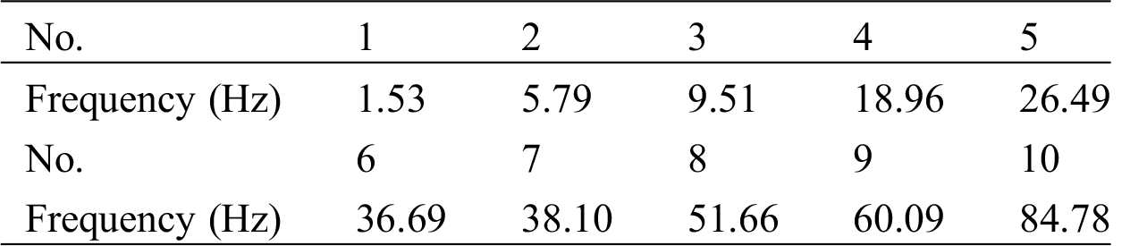
The frequency range used for the simulation of swept frequency is from 1 to 500 Hz, where the multi-source concentrated forces are applied in three different directions. The first 10 natural frequencies of the structure are shown in Tab. 5.

Table 5: Structure natural frequency

Apply vertical loads at six force application points separately, as shown in Tab. 6. The load identification result is shown in Fig. 4, and the relative error of the identified load is shown in Fig. 5.

Table 6: Vertical load size

Figure 4: Recognition result of multi-source vertical forces in the range of 1–500 Hz (a) Force application point 1 (b) Force application point 2 (c) Force application point 3 (d) Force application point 4 (e) Force application point 5 (f) Force application point 6

Figure 5: Relative error of multi-source vertical forces identification in the range of 1–500 Hz

Table 7: Maximum relative error of vertical loads dentification

Table 8: Minimum relative error of vertical loads identification

From Figs. 4 and 5, it is found that within the excitation frequency range of 1–500 Hz, The GCV method can effectively identify the dynamic loads. From Fig. 5, it can be seen that the relative error of the identification at five frequencies (i.e., 1 Hz, 9.12 Hz, 17.24 Hz, 25.37 Hz and 37.55 Hz) is larger, and the relative error of the identified load at other frequencies is all within 10%. Comparing with Tab. 5, it can be found that these five frequencies with large relative errors in identifying loads are all near the natural frequency of the structure. When the frequency is close to the natural frequency, the structure will resonate so the load identification result is poor. Tabs. 7 and 8 show the maximum and minimum relative errors of the GCV method and the direct inversion identification load. From these two tables, it can be seen that when the structure is in resonance, the GCV method can effectively reduce the identification compared with the direct inversion. The relative error of the load.

Four longitudinal loads are applied on the structure at the same time, as shown in Tab. 9, and the loads are identified by the GCV method. The identification results are shown in Figs. 6 and 7.

Table 9: Longitudinal load size

Figure 6: Recognition result of multi-source longitudinal loads in the range of 1–500 Hz (a) Force application point 2 (b) Force application point 3 (c) Force application point 4 (d) Force application point 6

Figure 7: Relative error of multi-source longitudinal loads identification in the range of 1–500 Hz

Table 10: Maximum relative error of Longitudinal loads identification

Table 11: Minimum relative error of Longitudinal loads identification

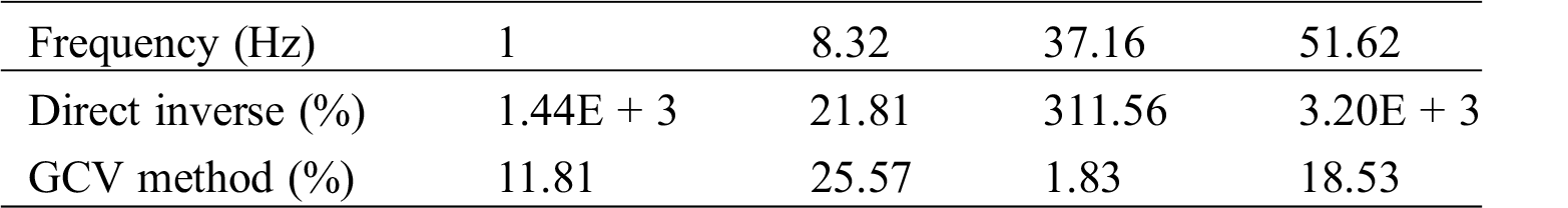
From Figs. 6 and 7, it is found that within the excitation frequency range of 1–500 Hz, The GCV method can effectively identify the loads. From Fig. 7, the relative errors at four frequencies (1 Hz, 8.23 Hz, 37.16 Hz and 51.62 Hz, respectively) are larger, and the relative error of the identified load at other frequencies is all within 10%. Compared with Tab. 5, it can be found that these four frequencies with large relative errors in identifying loads are all near the natural frequency of the structure. When the frequency is close to the natural frequency, the structure will resonate so that the load identification result is poor. In addition, we use the direct method and the GCV method to identify the load at these 4 scanning frequencies respectively, and compare the maximum relative error and minimum relative error of the identified load, as shown in Tabs. 10 and 11. From Tabs. 10 and 11, it can be seen that when the structure is in resonance, the GCV method can effectively reduce the identification error compared with direct inversion.

Four lateral loads are applied on the structure at the same time, as shown in Tab. 12, and are identified using GCV method. The identification results are shown in Figs. 8 and 9.

Table 12: Lateral load size

Figure 8: Recognition result of multi-source lateral loads in the range of 1–500 Hz (a) Force application point 1 (b) Force application point 2 (c) Force application point 3 (d) Force application point 6

Figure 9: Relative error of multi-source lateral loads identification in the range of 1–500 Hz

Table 13: Maximum relative error of lateral loads identification

Table 14: Minimum relative error of lateral loads identification

From Figs. 8 and 9, it is found that within the excitation frequency range of 1–500 Hz, the GCV method can effectively identify the loads. From Figs. 8 and 9, the relative errors at four frequencies (1 Hz, 8.23 Hz, 37.16 Hz and 51.62 Hz, respectively) are larger, and the relative error of the identified load at other frequencies is all within 10%. Compared with Tab. 5, it can be found that these four frequencies with large relative errors in identifying loads are all near the natural frequency of the structure. When the frequency is close to the natural frequency, the structure will resonate so the load identification result is poor. From Tabs. 13 to 14, it can be seen that when the structure is in resonance, the GCV method can effectively reduce the identification error compared with direct inversion.

6  Conclusion

This paper aims at identifying static/dynamic multi-source loads in stiffened plate structures by using strain responses. The conclusions obtained are as follows:

(1) The GCV, OCV and TSVD methods are used to identify static and dynamic load distributions on a reinforced plate structure, relying on strain responses. The recognition accuracy of the GCV method is proven to be higher than that of the TSVD and OCV methods.

(2) The GCV method is then used to identify the multi-source static loads applied in three different directions in the stiffened plate structure. The GCV method is able to identify the magnitudes of the loads with high accuracy, with relative error less than 5%.

(3) Under swept frequency excitation, the GCV method can effectively identify the multi-source load with relative errors less than 10%. In particular, near the natural frequency of the structure, the identification errors are much larger. However, compared with direct inversion, the GCV method is able to largely reduce the error of load identification.

Acknowledgement: The authors are grateful for the financial support provided by National Key R&D Program of China and National Natural Science Foundation of China.

Funding Statement: The authors received funding for this study from National Key R&D Program of China (2018YFA0702800), National Natural Science Foundation of China (12072056), the Fundamental Research Funds for the Central Universities (DUT19LK49), and Nantong Science and Technology Plan Project (No. MS22019016).

Conflicts of Interest: The authors declare that they have no conflicts of interest to report regarding the present study.

References

 1.  Jacquelin, E., Bennani, A., Hamelin, P. (2003). Force reconstruction: Analysis and regularization of a deconvolution problem. Journal of Sound & Vibration, 265(1), 81–107. [Google Scholar]

 2.  Law, S. S., Bu, J. Q., Zhu, X. Q., Chan, S. L. (2004). Vehicle axle loads identification using finite element method. Engineering Structures, 26(8), 1143–1153. [Google Scholar]

 3.  Yanyutin, E. G., Yanchevsky, I. V. (2004). Identification of an impulse load acting on an axisymmetrical hemispherical shell. International Journal of Solids and Structures, 41(13), 3643–3652. [Google Scholar]

 4.  Law, S. S., Bu, J. Q., Zhu, X. Q. (2005). Time-varying wind load identification from structural responses. Engineering Structures, 27(10), 1586–1598. [Google Scholar]

 5.  Pinkaew, T. (2006). Identification of vehicle axle loads from bridge responses using updated static component technique. Engineering Structures, 28(11), 1599–1608. [Google Scholar]

 6.  Gunawan, F. E., Homma, H., Kanto, Y. (2006). Two-step b-splines regularization method for solving an ill-posed problem of impact-force reconstruction. Journal of Sound and Vibration, 297(1–2), 200–214. [Google Scholar]

 7.  Kazemi, A. A., Bucher, C. (2015). Derivation of a new parametric impulse response matrix utilized for nodal wind load identification by response measurement. Journal of Sound and Vibration, 344, 101–113. [Google Scholar]

 8.  Jang, T. S., Baek, H., Han, S. L., Kinoshita, T. (2010). Indirect measurement of the impulsive load to a nonlinear system from dynamic responses: inverse problem formulation. Mechanical Systems and Signal Processing, 24(6), 1665–1681. [Google Scholar]

 9.  Thiene, M., Ghajari, M., Galvanetto, U., Aliabadi, M. H. (2014). Effects of the transfer function evaluation on the impact force reconstruction with application to composite panels. Composite Structures, 114, 1–9. [Google Scholar]

10. Renzi, C., Pezerat, C., Guyader, J. L. (2014). Local force identification on flexural plates using reduced finite element models. Computers & Structures, 144, 75–91. [Google Scholar]

11. Wentzel, H. (2013). Fatigue test load identification using weighted modal filtering based on stress. Mechanical Systems & Signal Processing, 40(2), 618–627. [Google Scholar]

12. Lee, M. H., Liu, Y. W. (2014). Input load identification of nonlinear tower structural system using intelligent inverse estimation algorithm. Procedia Engineering, 79, 540–549. [Google Scholar]

13. Cao, X., Sugiyama, Y., Mitsui, Y. (1998). Application of artificial neural networks to load identification. Computers & Structures, 69(1), 63–78. [Google Scholar]

14. Gupta, D. K., Dhingra, A. K. (2013). Input load identification from optimally placed strain gages using d-optimal design and model reduction. Mechanical Systems & Signal Processing, 40(2), 556–570. [Google Scholar]

15. Liu, Y., Shepard, W. S. (2005). Dynamic force identification based on enhanced least squares and total least-squares schemes in the frequency domain. Journal of Sound & Vibration, 282(1–2), 37–60. [Google Scholar]

16. Jian, Q. B., Xiang, S. L., Qun, X. Z. (2005). Moving loads identification based on generalized orthogonal function and regularization technique. Journal of Vibration, Measurement & Diagnosis, 1, 36–39. [Google Scholar]

17. Han, X., Jie, L. (2009). A computational inverse technique for reconstruction of multisource loads in time domain. Chinese Journal of Theoretical and Applied Mechanics, 41(4), 595–602. [Google Scholar]

18. Liu, J., Han, X., Jiang, C., Ning, H. M. (2011). Dynamic load identification for uncertain structures based on interval analysis and regularization method. International Journal of Computational Methods, 8(4), 1–17. [Google Scholar]

19. Liu, J., Can, X., Fan, L. (2015). Uncertain inverse method based on λ-PDF and first order second moment. Journal of Mechanical Engineering, 51(20), 135–143. [Google Scholar]

20. Granger, S., Perotin, L. (1999). An inverse method for the identification of a distributed random excitation acting on a vibrating structure part 1: Theory. Mechanical Systems and Signal Processing, 13(1), 53–65. [Google Scholar]

21. Perotin, L., Granger, S. (1999). An inverse method for the identification of a distributed random excitation acting on a vibrating structure part 2: Flow-induced vibration application. Mechanical Systems & Signal Processing, 13(1), 67–81. [Google Scholar]

22. Pézerat, C., Guyader, J. L. (2000). Force analysis technique: Reconstruction of force distribution on plates. Acta Acustica united with Acustica, 86(2), 322–332. [Google Scholar]

23. Pézerat, C., Guyader, J. L. (2007). Reconstruction of a distributed force applied on a thin cylindrical shell by an inverse method and spatial filtering. Journal of Sound and Vibration, 301(3–5), 560–575. [Google Scholar]

24. Zhong, X. L., Feng, C. (2006). Identification of moving loads on bridges using a grillage model. China Civil Engineering Journal, 39(12), 83–87. [Google Scholar]

25. Trabelsi, H., Abid, M., Taktak, M., Fakhfakh, T. (2014). Reconstruction of the unsteady rotating forces of fan’s blade from far-field sound pressure. Applied Acoustics, 86, 126–137. [Google Scholar]

26. Busby, H. R., Trujillo, D. M. (1997). Optimal regularization of an inverse dynamics problem. Computers & Structures, 63(2), 243–248. [Google Scholar]

27. Choi, H. G., Thite, A. N., Thompson, D. J. (2007). Comparison of methods for parameter selection in Tikhonov regularization with application to inverse force determination. Journal of Sound & Vibration, 304(3–5), 894–917. [Google Scholar]

28. Allen, D. M. (1974). The relationship between variable selection and data agumentation and a method for prediction. Technometrics, 16(1), 125–127. [Google Scholar]

29. Golub, G. H., Wahba, H. G. (1979). Generalized cross-validation as a method for choosing a good ridge parameter. Technometrics, 21(2), 215–223. [Google Scholar]

This work is licensed under a Creative Commons Attribution 4.0 International License, which permits unrestricted use, distribution, and reproduction in any medium, provided the original work is properly cited.