Health Monitoring
| Structural Durability & Health Monitoring |
DOI: 10.32604/sdhm.2021.012316
ARTICLE
Condition Evaluation in Steel Truss Bridge with Fused Hilbert Transform, Spectral Kurtosis, and Bandpass Filter
1National Institute of Technology, Hamirpur, 177005, India
2Entrepreneurship Development and Industrial Coordination Department, National Institute of Technical Teachers Training and Research, Chandigarh, 160019, India
3Himachal Pradesh Public Works Department, Kangra, 176001, India
*Corresponding Author: Anshul Sharma. Email: anshul.s@nith.ac.in
Received: 25 June 2020; Accepted: 26 February 2021
Abstract: This study is concerned with the diagnosis of discrepancies in a steel truss bridge by identifying dynamic properties from the vibration response signals of the bridges. The vibration response signals collected at bridges under three different vehicular speeds of 10 km/hr, 20 km/hr, and 30 km/hr are analyzed using statistical features such as kurtosis, magnitude of peak-to-peak, root mean square, crest factor as well as impulse factor in time domain, and Stockwell transform in the time-frequency domain. The considered statistical features except for kurtosis show uncertain behavior. The Stockwell transform showed low-resolution outcomes when the presence of noise in the recorded vibration responses. The elimination of noise and extraction of meaningful dynamic properties from the vibration responses is done by applying a new method which comes from the fusion of Hilbert transform with Spectral kurtosis and bandpass filtering. The outcomes obtained from Hilbert transform processed residual signals which are further filtered using bandpass filter show more robustness and accuracy in characterizing bridge modal frequencies from the noisy vibration responses. The proposed method produces a high-resolution frequency response which can unveil the joint discrepancy in the bridge structure.
Keywords: Steel bridge; damage detection; stockwell transform; hilbert transform; spectral kurtosis; bandpass filter
Notations
| | Angular frequency of |
| | root mean square |
| | Complex envelope |
| | the scaling factor used to vary gaussian window width |
| | The envelope of |
| | Fourier transform of signal |
| | Spectral kurtosis |
| | Gaussian window |
| | time averaging operator |
| | Hilbert transform |
| | translation parameters |
| | maximum peak values |
| | window length |
| | Phase angle |
The damage detection using vibration-based signal processing techniques in bridges has been widely applied in recent decades [1]. The advanced signal processing techniques have been applied to solve various problems such as damage detection, structural integrity determination, image processing in concrete, crack determination, ground penetrating radars, etc. The irregularities in an ideal structure introduced degrades the functioning of the structure [2–5]. The literature has reported some common reasons which cause irregularity introduction in a bridge that includes vehicular accidents, fatigue stresses development, connection loosening, operational vicinity environmental conditions variations, aging of various members, etc. [6] which imbalances the geometry, the integrity of the structure and reduces its serviceable lifespan. The cyclic fatigue stresses developed overcomes the strength of the bridge members and develops deficiencies in a bridge [7,8].
Various bridge health monitoring measures were taken in past to detect these structural deficiencies as early as possible and provide suitable countermeasures associated with the particular problem such that there can be an enhancement in the service span of the bridge [9]. The non-destructive techniques (NDTs) based on vibration response utilization give minimum damage to the structure while testing and accurately determines the health state of the structure in real-time [10,11]. The demand for fast irregularity detection in complex structures has attracted many researchers in pursuing bridge health monitoring. The experimental study of bridge health monitoring using vibration methods includes the collection of the bridge’s vibration response signals with a network of sensors mounted at specific locations of the bridge [12,13]. A huge data set is obtained which further requires large computational time and a skilled person to evaluate the outcomes correctly and provide meaningful information about the existing state of the bridge [14]. Various signal processing techniques have been developed over time to deal with this problem and provide robust results in time, frequency, and time-frequency domains.
The time-domain analysis includes the use of statistical and stochastic features in performing time-history signals analysis [15–17]. In this investigation, the statistical features of root mean square (RMS), Crest Factor, Kurtosis, Impulse Factor, and Magnitude of Peak-to-Peak, are applied to analyze the measured temporal vibration responses of bridges. The frequency-domain analysis converts the signals in the frequency domain and the visualization is done in amplitude versus frequency of the signal [18]. The Fast Fourier transform (FFT) application provides frequency domain visualization of the original vibration signal responses. The time-frequency analysis such as wavelet transform and S transform enables us to visualize the signal in both time and frequency planes simultaneously [19].
The loosening of joint connections in a bridge produces transient variation in vibration responses due to alterations in resonant modal properties such as natural frequencies etc. of the bridge [20]. The spectral kurtosis (SK) is a proposed tool which has a sensitive feature of determining non-stationary patterns and is able to indicate the frequencies occurring in a signal. Furthermore, the development of detection filters using spectral kurtosis makes it easy to extract faulty signals from added unwanted white noise. The literature provides a suitable example of spectral kurtosis in the field of bearing fault detection [21], marine propeller [22], wind turbine [23], etc. The change of bridge structure from its ideal health condition to abnormal state can be generally reflected through spectral kurtosis analysis as the damage signature arising from the measured vibration response signals.
The present study clarifies the limitations of statistical (time domain), and S-transform (time-frequency domain) techniques in eliminating noise involved in the recorded vibration response signals from the steel truss bridge, and demonstrates the proposed technique of analyzing recorded vibration response signals at different vehicular speeds through combined Hilbert transform, Spectral kurtosis and bandpass filtering technique is efficient in extracting modal frequencies of the steel truss bridge. The obtained modal frequencies are used to determine the location of discrepancies in the steel truss bridge. The structurally deficient nodes showed either missing or low amplitude of modal frequencies due to loss of stiffness in the joining members at a particular location.
2 Description of the Steel Truss Bridge
The through-type steel truss bridge considered for the study is a simply supported bridge having a span of 40 m with a single lane carriageway. It is supported by the roller at one end and hinged at another end. There is an equal spacing of 4 m interval among the vertical members along the span of the bridge as shown in Fig. 1. The diagonal and vertical members are built-up sections formed of four angles with each set of two angles joined toe to toe. The bottom and top horizontal members are formed from two-channel sections attached back to back. The longitudinal members and crossbeams comprise ISMB 450 and ISMB 550. The use of gusset plates with riveted connections is done to join the members of both the trusses. The deck of the steel bridge has a 175 mm thick reinforced concrete slab covered with a wearing coat of 75 mm thickness. The width of the carriageway is 5 m along adjoined with 225 mm × 225 mm side curbs. A grid of longitudinal members and crossbeams having a spacing of 1.4 m × 4 m is used to support the whole deck of the bridge. The steel bridge experimentation is conducted to check the behavior of joints for any disparity occurrence along both upstream and downstream trusses of the bridge. The experimental procedure consists of collecting ambient and forced vibrational responses developed due to movement of the vehicle in to-and-fro motion over the bridge with the help of sensors placed at the bridge. The measurements of accelerations were done in vertical directions at 18 node locations with a total of 6 sets of sensors placement [24]. The cyclic shifting of non-reference sensors is done to collect vibrational data. A reference sensor (blue arrow sensor) and three movable sensors (red arrow sensor) for any particular sensor set are shown in Fig. 2. The downstream nodes were named as 1, 2…, and 11 and upstream nodes as 12, 13…, and 22 with nodal points of 1, 2, 11, and 22 at supports. The acceleration vibration responses of steel truss bridge at different vehicular movement speeds of 10 km/hr, 20 km/hr, and 30 km/hr are recorded. The selection of vehicular speed opted for experimentation is based on the condition of probable minimum and maximum speeds of the vehicle which can be achieved such that all the modes of steel bridge get excited. The instrument setup is the same for the varying speeds of the vehicle and the sampling frequency of 200 sps is considered while performing the experiments. The first three analytical frequencies of the steel truss bridge model are 4.56 Hz, 10.44 Hz, and 16.66 Hz, respectively [24]. The detailed description of all components of a real-time steel truss bridge, testing procedure, and analytical study is provided in previous studies [24,25], respectively.
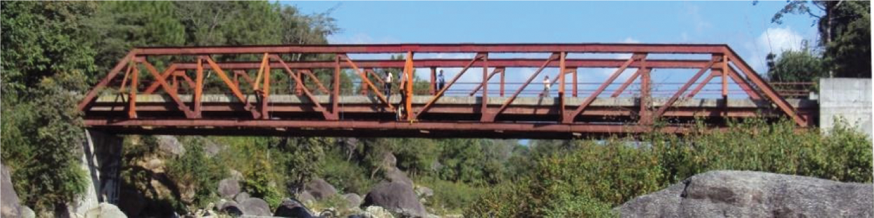
Figure 1: Real-time 40 m steel truss bridge
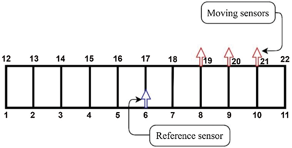
Figure 2: Typical set of sensors layout for vibration measurement
3 Signal Processing Techniques
A summary of the definitions, process, and application of each technique used in the recorded vibration signal analysis are presented in this section. During the analysis, it has been found that the behavior of the nodes is random and the response hence is shown for all nodes under different signal processing techniques.
The time-domain analysis involves the computation of statistical features from the original data. Some of the popular statistical features used in the study include Crest Factor, Impulse Factor, Kurtosis, and magnitude of Peak-to-Peak [17]. The statistical features of the recorded vibration signals from considered steel truss bridge at different vehicular speeds of 10 km/hr, 20 km/hr, and 30 km/hr have been determined. It has been observed that as the vehicular speed increases a noticeable variation occurs in various statistical features (Crest Factor, Kurtosis, Impulse Factor, and Peak-to-Peak).
For any vibration signal y(i) in the time domain, with i = 1, 2, …, n, where n represents the different data points present in the signal. The root mean square (
Crest Factor (
where the maximum peak values (
The crest factor feature showed marginal variation at different nodes of the bridge as shown in Fig. 3. The nodes 4 and 10 in the downstream truss and 13, 14, 17, 18, and 19 in the upstream truss behaved ideally and followed an absolute increasing pattern with the increase in vehicular speed. However, nodes 2, 3, 5, 7, 8, and 9 in the downstream truss and 15, 16, 20, and 21 in the upstream truss exhibited no clear pattern with the variation in vehicular speed. The crest factor feature lacks confidence for determining the particular behavior as the pattern for a large number of nodes is not obtained with much clarity.
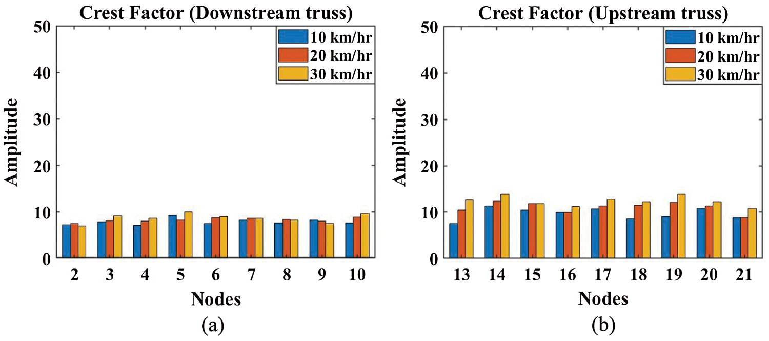
Figure 3: Crest factor feature plots (a) Downstream truss (b) Upstream truss
Kurtosis (
The kurtosis feature showed a significant irregular rise in amplitude at 6, 7, and 8 downstream nodes for both 10 km/hr and 30 km/hr vehicular speeds, while the amplitude of these nodes decreased suddenly with respect to other nodes for 20 km/hr vehicular speed. This indicates the possibility of having structural flexibility deficiencies at these locations. The nodes in the upstream truss exhibit absolute ascending order variation in amplitudes except for marginal variation in nodes 14 and 16 as shown in Fig. 4. The kurtosis feature is able to show the intactness of the nodes 2, 3, 4, 5, 9, and 10 in downstream truss and nodes 13, 15, 17, 18, 19, 20, and 21 in upstream truss as an absolute increase in kurtosis amplitude with the increase in vehicular speed.
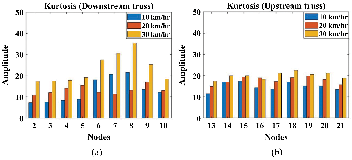
Figure 4: Kurtosis feature plots (a) Downstream truss (b) Upstream truss
Impulse Factor (
The impulse factor values on downstream truss showed an absolute increasing trend for nodes 3, 4, 6, 7, and 10 while on upstream truss no definite pattern is observed as shown in Fig. 5. The downstream nodes 8 and 9 showed an irregular pattern in their behavior with the rise in vehicular speeds. The impulse factor feature lacks in showing any clear pattern particularly for the behavior of the upstream nodes and hence no decisive conclusion for identifying the deficient nodes was not achieved.
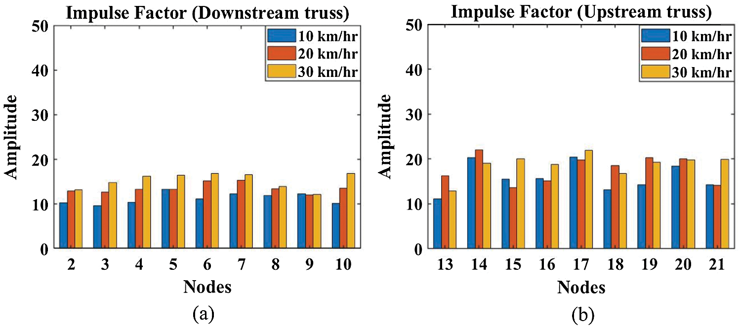
Figure 5: Impulse factor feature plots (a) Downstream truss (b) Upstream truss
Magnitude of Peak-to-Peak (
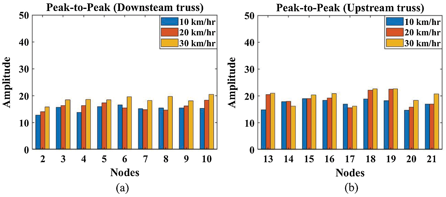
Figure 6: Peak-to-Peak feature plots (a) Downstream truss (b) Upstream truss
The idea behind calculating some popular statistical features is to investigate raw signals in the time domain and identify nodes showing irregular behavior. Except for kurtosis other features were unable to give any significant variation in the behavior of nodes of the bridge. The staggering difference between the upstream and downstream truss nodes response is due to varying stiffness in members of the trusses. From the graphs, it is observable that maximum significant variation occurs in nodes 6, 7, and 8 and the kurtosis feature shows a reasonable change hence for further analysis kurtosis is considered. The downstream nodes 6, 7, and 8 showed peculiar behavior in comparison to all other nodes. However, magnitude of Peak-to-Peak also indicates a peculiar pattern at nodes 6, 7, and 8 but kurtosis is comparatively more distinct. However, on the upstream truss, the kurtosis results at all the nodes follow a similar pattern whereas the magnitude of Peak-to-Peak feature show randomness and do not yield any useful information.
3.2 Time-Frequency Domain Analysis
The Fourier transform has the limitation of simultaneously visualizing frequency and time and it is also not suitable for non-stationary signals [28–30]. Hence, time-frequency domain analysis is a prominent technique to determine the variation in frequency content present in signal with respect to time. Various time-frequency techniques such as Wigner–Ville Distribution (WVD), Gabor–Wigner transform, Wigner transform, Short Time Fourier Transform (STFT), Wavelet transform, Stockwell transform, etc., have been developed over time with their suitable distinct application [31,32]. The time-frequency domain analysis is performed using the Stockwell transform which gives better resolution over the WVD and STFT in the present study.
3.2.1 Stockwell Transform (S Transform)
Stockwell transform involves combined elements of both Short Time Fourier transform (STFT) and wavelet transform (WT) that gives outcome in the time-frequency spectrum [33]. Stockwell transform solves the problem of representing any signal simultaneously in both time and frequency domains by proposing a suggestion of opting for a base function with a movable and scalable gaussian window. The increase in the width of the time window makes the resolution of low frequencies higher and with the decrease in window size higher frequencies can be seen with high resolution [34].
The Short-Time Fourier Transform (
where, f = frequency and r, t = time variables
The uncertainty principle states that the product of time-bandwidth cannot be reduced without limits. The Gaussian window (
where,
‘
The new base function obtained is shown as Eq. (9)
where
The mathematical expression of S-transform is shown as Eq. (10)
The inverse S-transform can be expressed as Eq. (11)
where
The plots of S-transform have been shown for downstream nodes 2, 6, 7, and 8 at different vehicular speeds in Fig. 7. The frequencies obtained in the vicinity of the first three analytically obtained modal frequencies (4.56 Hz, 10.44 Hz, and 16.66 Hz) are determined.
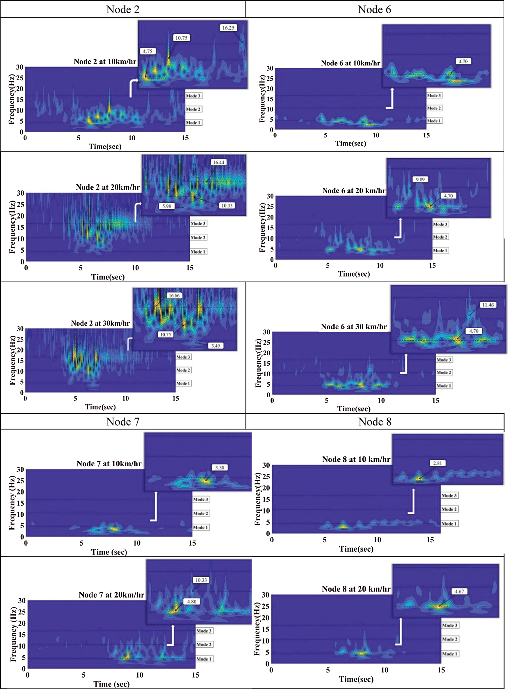

Figure 7: S-Transform plots for downstream nodes 2, 6, 7, and 8 of the steel truss bridge)
For downstream nodes, 1st, 2nd and 3rd modal frequencies at vehicular speeds of (a) 10 km/hr are in the range of 2.81 Hz to 16.75 Hz, 7.25 Hz to 11.33 Hz, and 16.25 Hz to 16.99 Hz, respectively (b) 20 km/hr are in the range of 4.67 Hz to 6.57 Hz, 8.28 Hz to 10.66 Hz and 14.75 Hz to 16.66 Hz, respectively (c) 30 km/hr are in the range of 3.49 Hz to 4.70 Hz, 7.98 Hz to 12.57 Hz and 16.56 Hz to 16.75 Hz, respectively.
The detailed values of all the frequencies obtained for downstream nodes around 1st (4.56 Hz), 2nd (10.44 Hz), and 3rd (16.66 Hz) analytical modal frequencies from Stockwell transform at all vehicular speeds are shown in Tab. 1, respectively.
Table 1: Frequencies obtained for downstream nodes from Stockwell transform nearby analytical modal frequencies
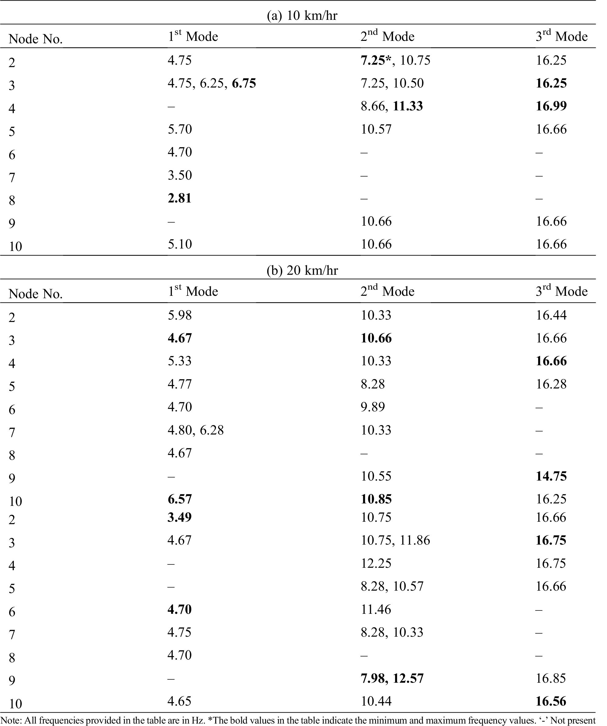
The mean of frequencies obtained around 1st, 2nd, and 3rd modes for 10 km/hr vehicular speed are 4.92 Hz, 9.74 Hz, and 16.58 Hz, respectively. For 20 km/hr vehicular speed are 5.31 Hz, 10.15 Hz, and 16.17 Hz, respectively. For 30 km/hr vehicular speed are 4.49 Hz, 10.46 Hz, and 16.71 Hz, respectively.
The plots of S-transform have been shown for upstream nodes 13, 15, 16, and 18 at different vehicular speeds in Fig. 8.
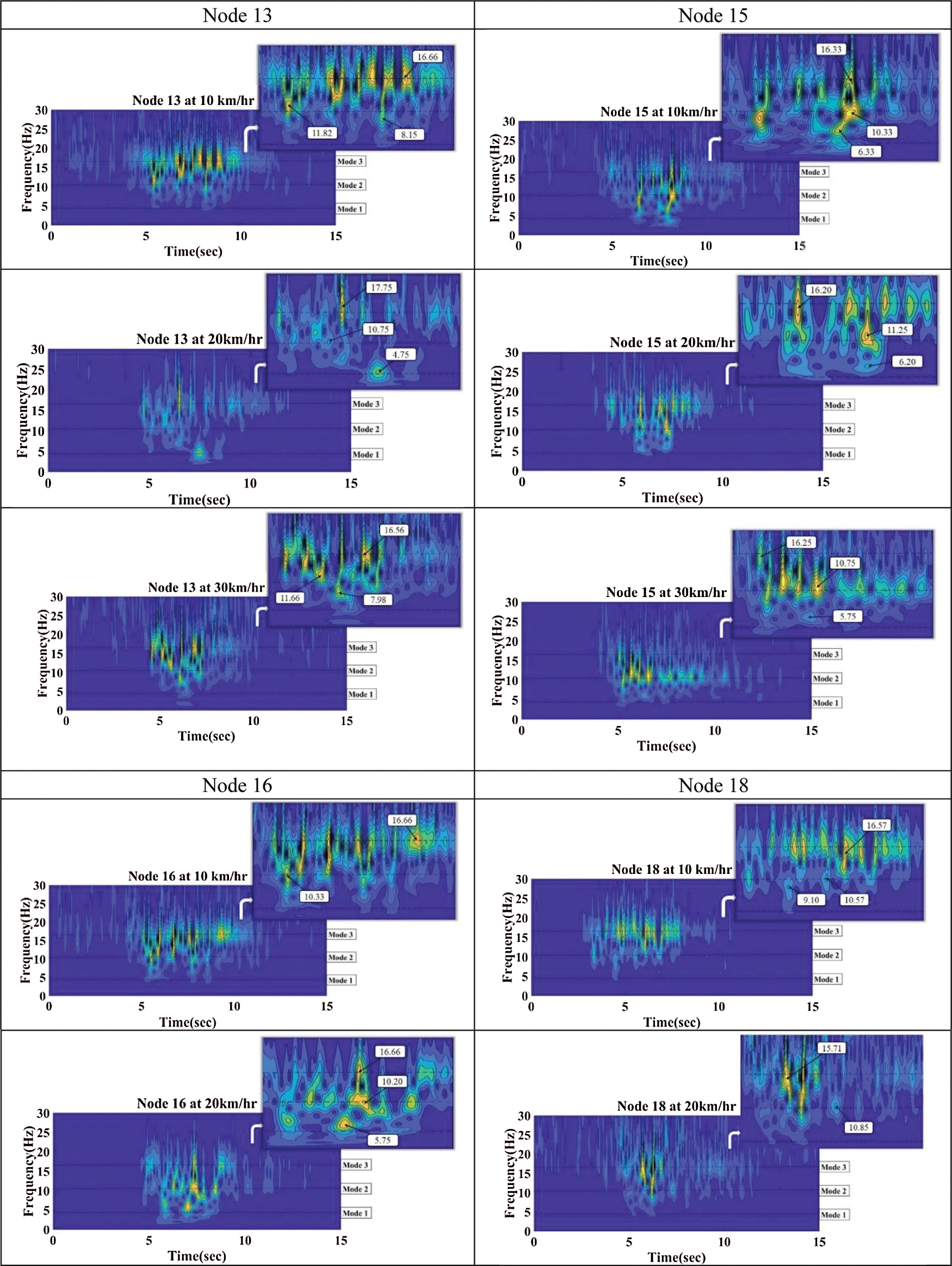
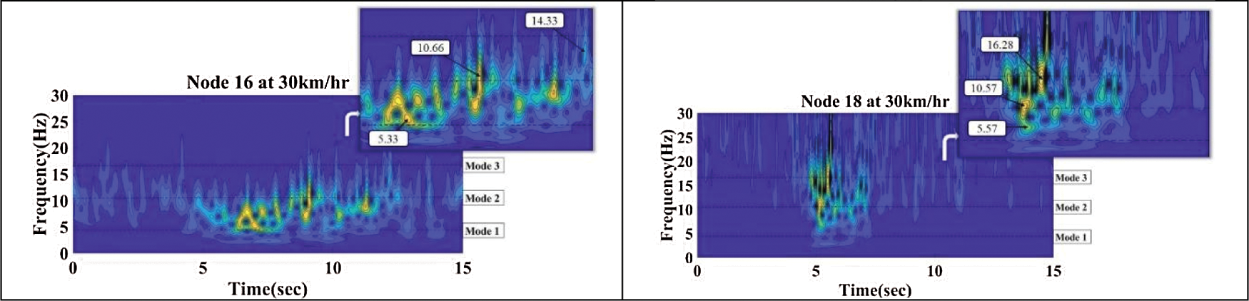
Figure 8: S-Transform plots for upstream nodes 13, 15, 16, and 18 of the steel truss bridge
For upstream nodes, 1st, 2nd and 3rd modal frequencies at vehicular speeds of (a) 10 km/hr are in the range of 4.66 Hz to 6.98 Hz, 7.98 Hz to 12.04 Hz, and 14.33 Hz to 16.86 Hz, respectively (b) 20 km/hr are in the range of 4.75 Hz to 5.75 Hz, 7.50 Hz to 12.55 Hz and 13.25 Hz to 17.75 Hz, respectively (c) 30 km/hr are in the range of 5.33 Hz to 7.98 Hz, 8.34 Hz to 12.25 Hz and 14.55 Hz to 17.75 Hz, respectively.
The values of all the frequencies obtained for upstream nodes around 1st (4.56 Hz), 2nd (10.44 Hz), and 3rd (16.66 Hz) analytical modal frequencies from Stockwell transform at all vehicular speeds are shown in Tab. 2, respectively.
Table 2: Frequencies obtained for upstream nodes from Stockwell transform nearby analytical modal frequencies
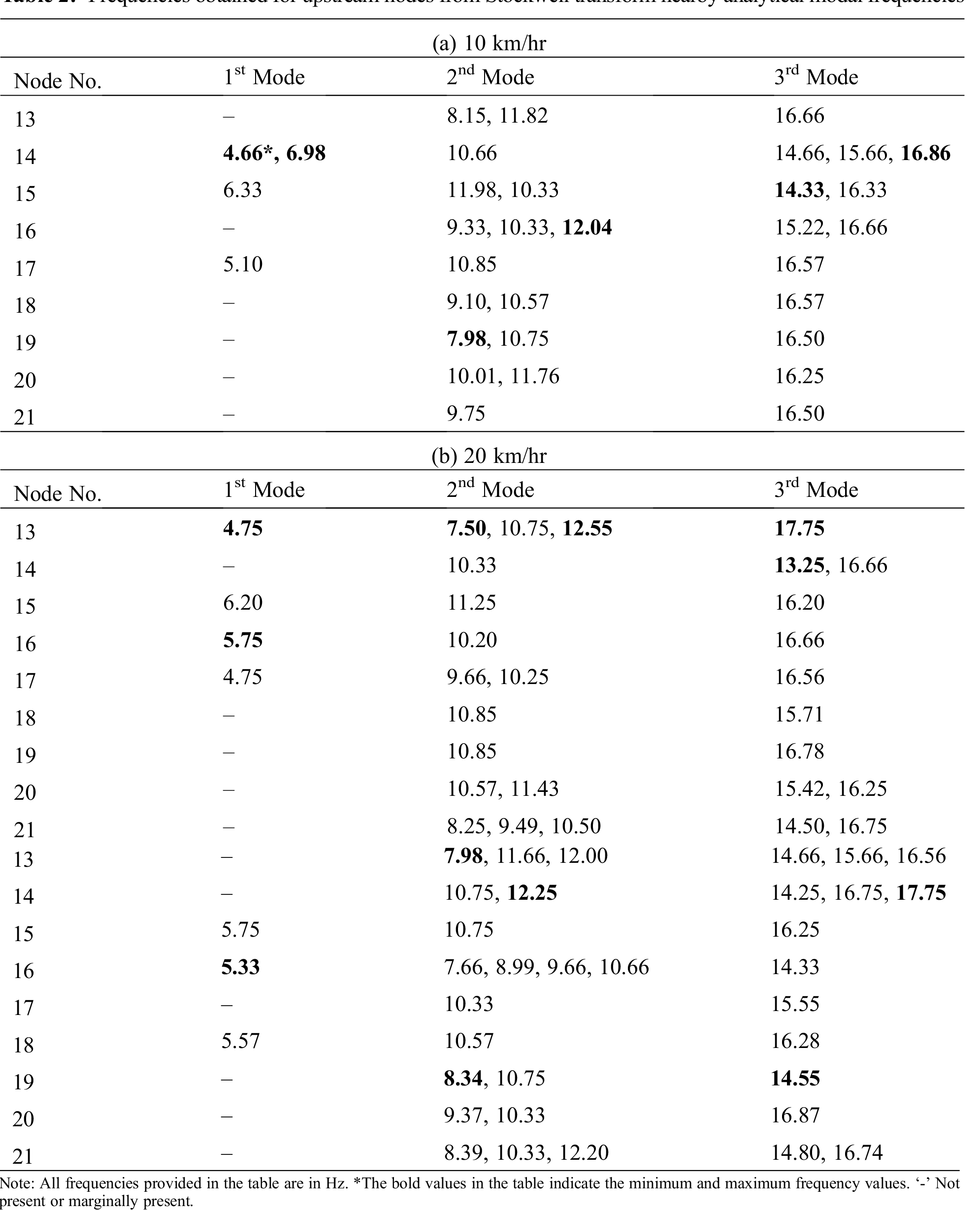
The mean of frequencies obtained around 1st, 2nd, and 3rd modes for 10 km/hr vehicular speed are 5.77 Hz, 10.34 Hz, and 16.06 Hz, respectively. For 20 km/hr vehicular speed are 5.36 Hz, 10.30 Hz, and 15.99 Hz, respectively. For 30 km/hr vehicular speed are 5.55 Hz, 10.16 Hz, and 15.79 Hz, respectively.
From the Stockwell transform plots it is concluded that at different vehicular speeds the frequencies of downstream and upstream nodes are not exactly same. The resolution of output plots showing the frequencies present in the vibration response signals got improved with the application of Stockwell transform with respect to time features respectively. However, the presence of noise in the vibration signals generated unwanted frequencies in the vicinity of desired modal frequencies. The nodes 6, 7, and 8 in downstream truss showed undesired behavior with the presence of higher intensity frequencies only around 1st mode at all the vehicular speeds.
To ensure that there exists partial flexibility in the joints at these locations further denoising of the vibration signals is required. Various studies are showing a broader range of areas of application of Hilbert transform on noisy vibration signals for obtaining better visualization of hidden frequencies [35–42]. In the present study, the efficiency of fused Hilbert transform with spectral kurtosis and bandpass filter in obtaining the modal frequency of a steel truss bridge is shown. The Hilbert transform is the relationship between the real and imaginary parts of the FFT of a one-sided function. Hilbert transform
where,
Hilbert transform is a frequency independent time domain involution that maps real time-domain value into another value. It is also called 90° phase shifter and does not affect the non-stationary characteristics of a modulating signal. This can be obtained mathematically by the following Eq. (13)
where,
where,
From the time domain analysis performed earlier it is known that the kurtosis feature shows better performance than others, hence the signal obtained after Hilbert transform having the highest kurtosis value is selected to obtain a spectral response. The spectral kurtosis provides the highest kurtosis value, frequency present along with its duration in the signal. Further, the bandpass filter is used to refine the final outcome vibration signal. The modal frequencies are obtained which are further utilized to identify the bridge nodes having discrepancies, respectively.
After the analysis of popular statistical features, and improved method in time-frequency, i.e., S-transform. The identification of flexible nodes requires more confidence. From the performed analysis it has been concluded that time-domain analysis only gives the identification of response of speed variation. The time-frequency analysis gives more information regarding the condition of nodes from frequencies obtained with poor resolution due to the presence of noise in vibration signals measured from the bridge. However, by using previously established techniques, due to the presence of noise some nodes not able to give a clear understanding of the node which may mislead the interpretation. Thus, a methodology is proposed that is efficiently able to remove the noise and successfully provide a clear view of the present fundamental modal frequencies of the bridge. The methodology adopted here is shown in the flowchart in Fig. 9.
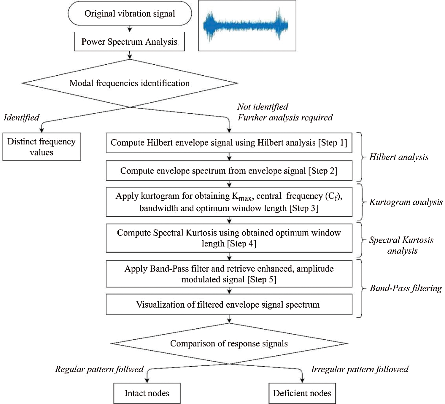
Figure 9: Flowchart of the adopted methodology
Step 1: Initially power spectrum analysis is performed and then Hilbert transform is computed.
Step 2: The Hilbert envelope spectrum is calculated from the Hilbert envelope signal to identify the modal frequencies. The Hilbert envelope spectrum analysis was performed to present the hidden dynamic information which spectral analysis fails to depict. The typical envelope signal and envelope spectrum plots are shown in Figs. 10a and 10b, respectively. The Hilbert envelope spectrum limits in showing significant peaks due to the masking of external noise.
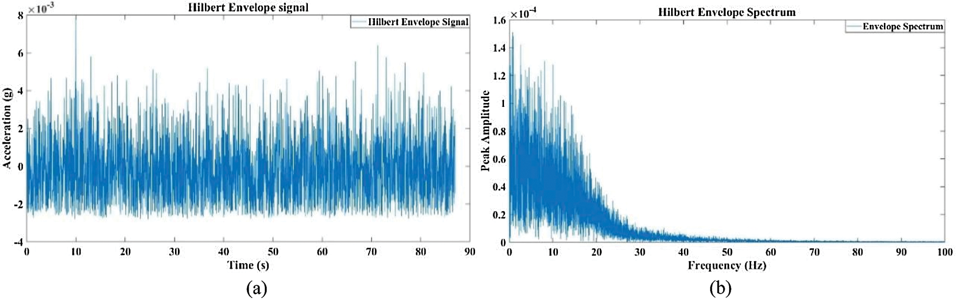
Figure 10: Hilbert envelope (a) of signal and (b) its spectrum
The visualization of the contaminated signal in the time domain along with the computation of kurtosis of the signal was done.
Step 3: Kurtosis is a statistical measure that defines how heavily the tails of distribution differ from the tails of a normal distribution as shown in Fig. 11 [43]. In other words, kurtosis identifies whether the tails of a given distribution contain extreme values. In our case, lower kurtosis means the low extreme value which indicates the node is not vibrated more due to its stiffness. The selection of signals with the highest kurtosis was made with kurtogram plots. The kurtosis shows the impulsiveness present in a signal. The occurrence of large impulsiveness shows the inclusion of more faulty signal features hence enhancing the signal-to-noise ratio through Hilbert transform makes it a vital step before performing envelope spectral analysis. The local computation of kurtosis within frequency bands was done with kurtogram evaluation and spectral kurtosis application [44]. The kurtogram indicates the central frequency of the frequency band with proper bandwidth and highest kurtosis values depiction. The kurtogram also suggests the optimal window length for calculating the spectral kurtosis of the original signal as shown in Fig. 12.
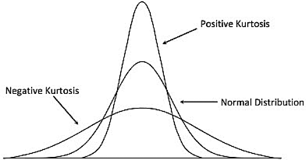
Figure 11: The normal distribution, positive kurtosis and negative kurtosis [43]
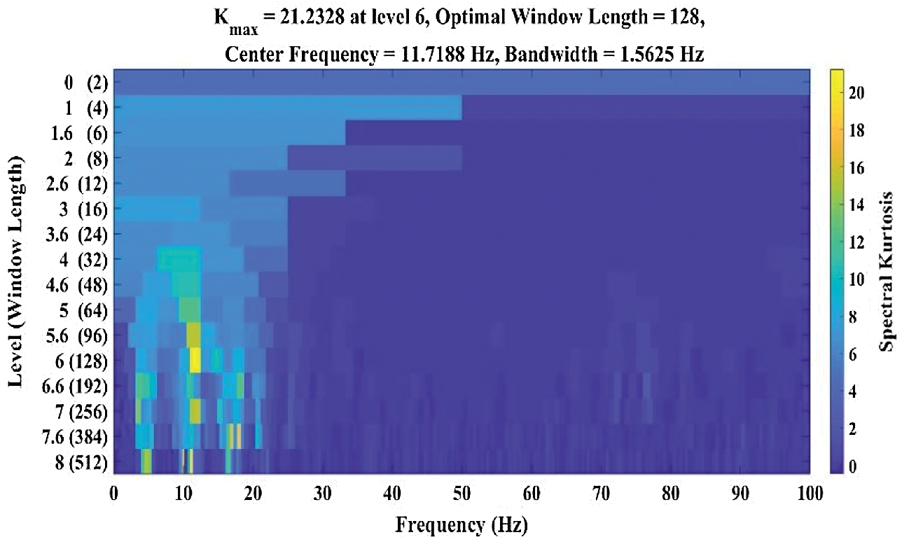
Figure 12: Kurtogram plot of a typical node
The typical spectrogram of spectral kurtosis is shown in Fig. 13. The presence of central frequency at 11.72 Hz is shown in the plot.
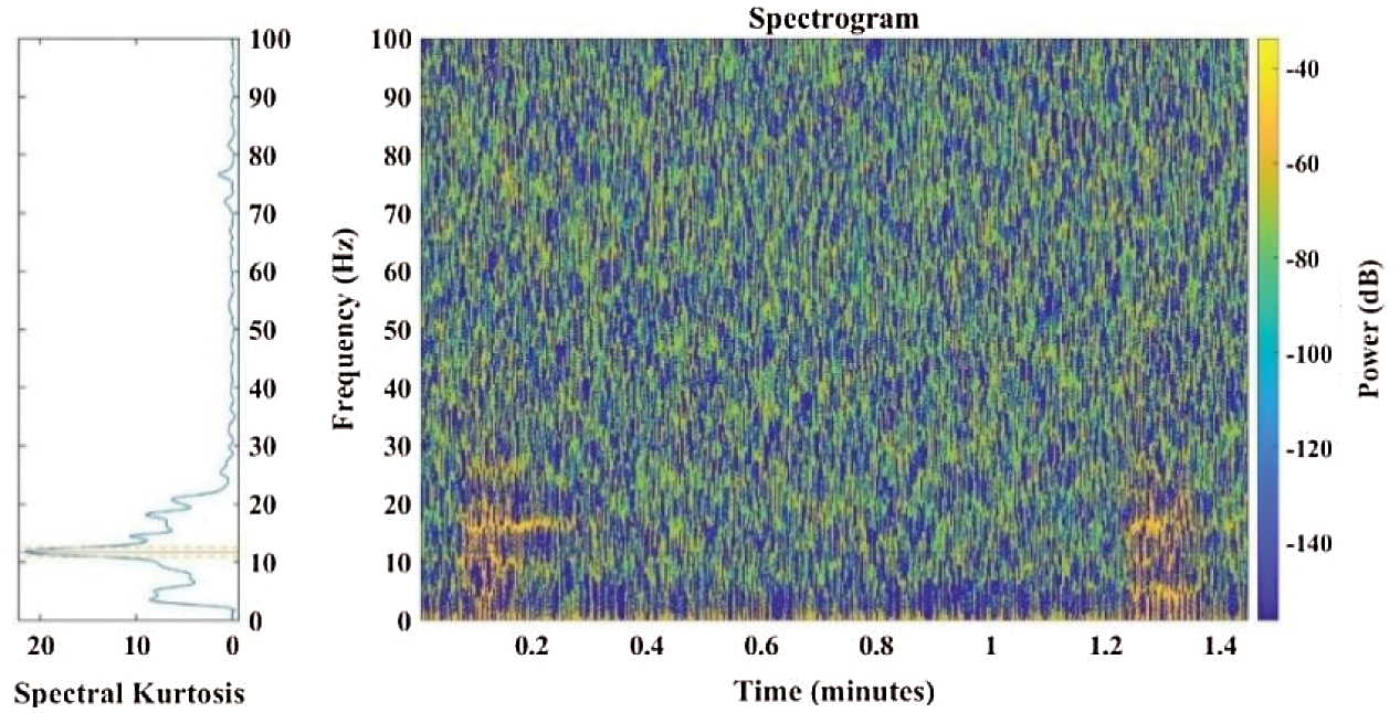
Figure 13: Spectrogram plot of spectral kurtosis of a typical node
Step 4: The Spectral Kurtosis is applied to the specified window length obtained from kurtogram plots. The concept of spectral kurtosis (
where
“−2” removes the complexity of the signal
The complex envelope (
where
The complex envelope
4.1 Application of the Developed Methodology
The refined spectral kurtosis plots for typical nodes 2 and 6 at different vehicular speeds of 10 km/hr, 20 km/hr, and 30 km/hr are shown in Fig. 14, respectively. The typical nodes 2 and 6 are selected to show the variation in spectral kurtosis plots for intact and damaged nodes of the bridge. The intact nodes 2, 3, 4, 5, 9, and 10 showed variation in frequency from 30 Hz to 40 Hz with the increase in vehicular speed from 10 km/hr to 30 km/hr, respectively. The nodes 6, 7, and 8 showed irregular behavior as the frequencies concentrated in the lower range up to 10 Hz only. This behavior raises suspicions about the intactness of nodes 6, 7, and 8, respectively. For upstream truss, all the nodes 13, 14… up to 21 followed a similar pattern of having frequencies up to 30 Hz at the lower vehicular speed of 10 km/hr whereas the spread of frequency range was up to 40 Hz for the vehicular speed 20 km/hr and 30 km/hr.
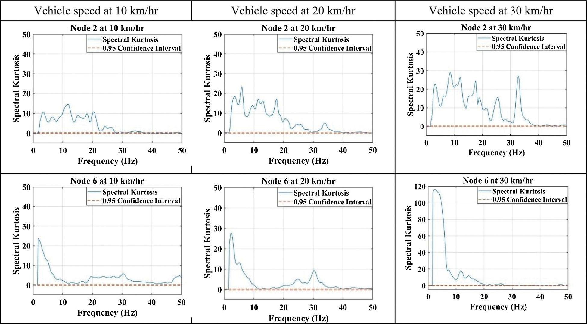
Figure 14: Spectral Kurtosis of typical nodes 2 and 6 of the steel truss bridge
It is concluded that all downstream and upstream nodes showed a high range of frequencies except for nodes 6, 7, and 8, respectively. This indicates that the Spectral Kurtosis values give a clear-cut indication of the consolidation in frequencies in the lower range for deficient nodes.
Step 5 Band-Pass filter is applied to the spectral kurtosis outcome signals for retrieving a more enhanced amplitude modulated signal. The low frequency and high frequency cut offs used in band pass filter for effective filtration of the noise from spectral kurtosis signal are 0 Hz to 35 Hz, respectively.
Fig. 15 shows the output of the bandpass filter where the original signal and filtered signal with their envelope are shown by blue and red signals. Figs. 16a and 16b shows the magnitude-squared coherence and cross spectrum phase plots respectively for typical node 6 for typical node 6 at 10 km/hr, 20 km/hr, and 30 km/hr vehicular speeds.
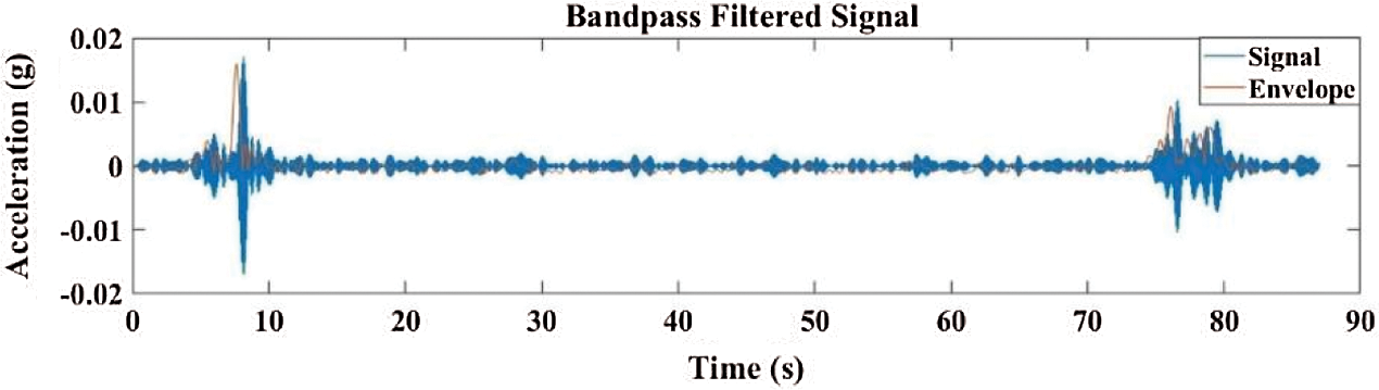
Figure 15: Band-Pass filtering plots at a typical node
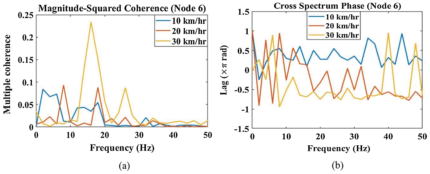
Figure 16: (a) Magnitude-squared coherence plots and (b) Cross spectrum phase plots for typical node 6 at 10 km/hr, 20 km/hr, and 30 km/hr vehicular speeds
The spectrum responses of downstream nodes from the proposed methodology at different vehicular speeds respectively are shown in Fig. 17. The 1st, 2nd and 3rd modal frequencies for vehicular speed of (a) 10 km/hr are in the range of 4.69 Hz, 10.94 Hz to 11.72 Hz, and 16.41 Hz to 17.20 Hz, respectively. (b) 20 km/hr are in the range of 3.91 Hz to 5.47 Hz, 8.59 Hz to 11.72 Hz, and 16.41 Hz to 17.97 Hz, respectively. (c) 30 km/hr are in the range of 3.91 Hz to 5.47 Hz, 10.16 Hz to 11.72 Hz, and 16.41 Hz, respectively.
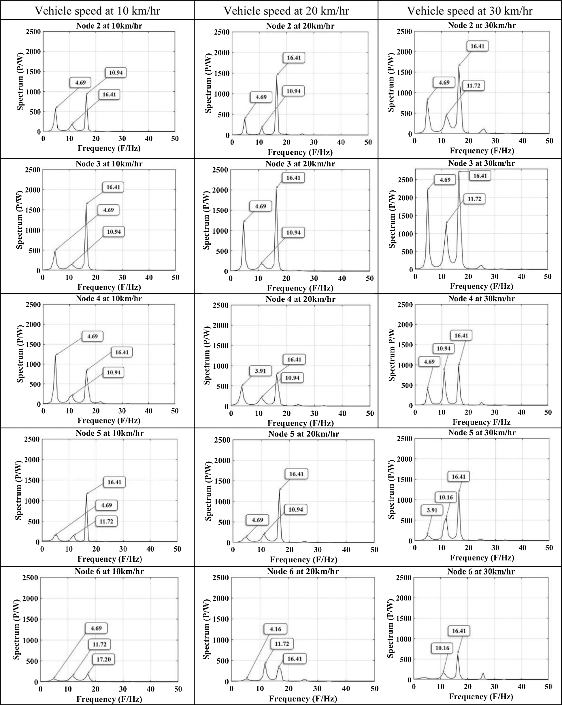
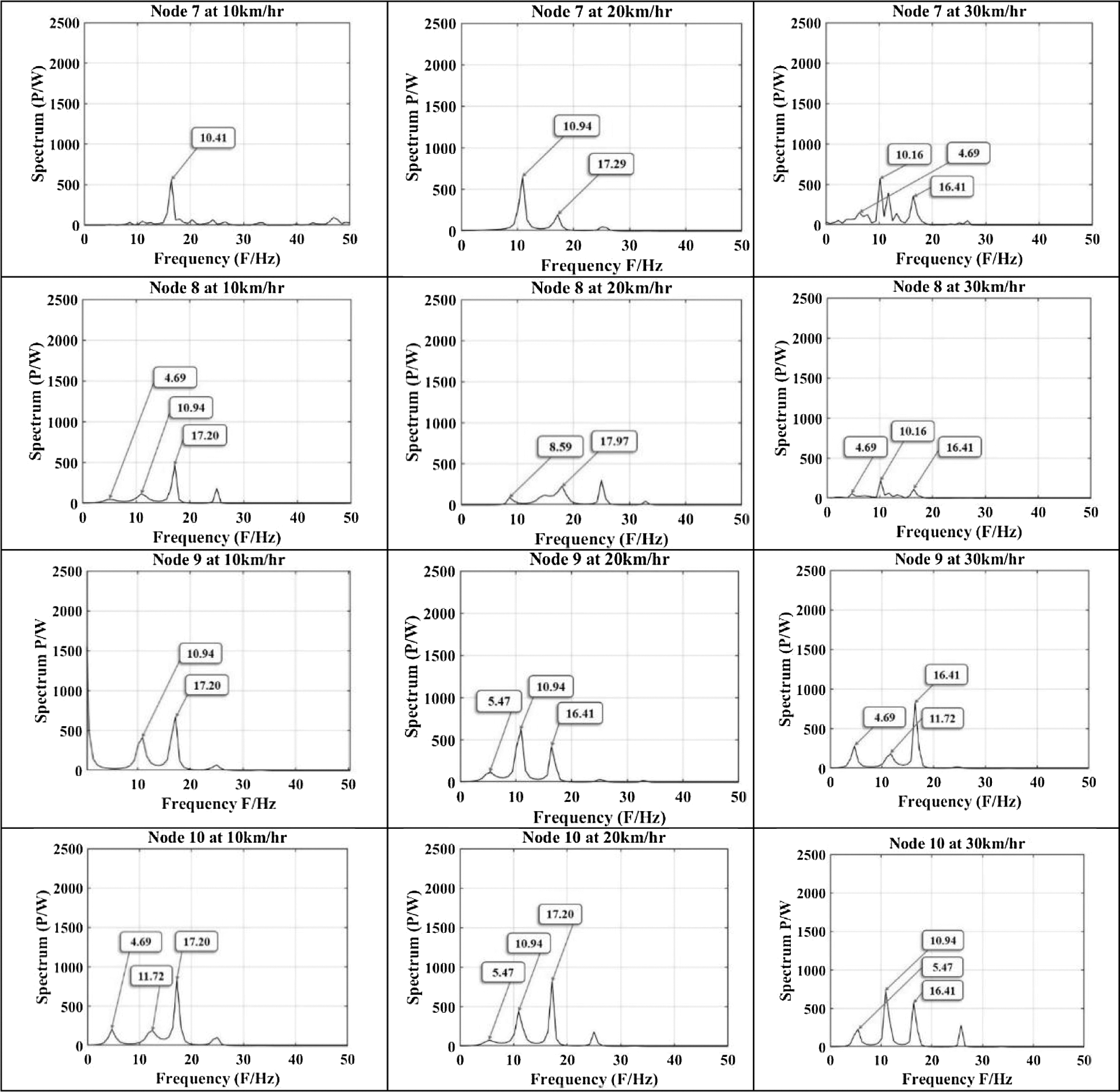
Figure 17: Proposed methodology outcomes for downstream nodes of the steel truss bridge
For the downstream nodes at 10 km/hr vehicular speed the 1st modal frequency is obtained for all the nodes except for nodes 7 and 9, respectively. The nodes 5, 6, and 8 showed a low amplitude of 1st modal frequency. The 2nd modal frequency is obtained with low amplitude for all the nodes except for nodes 7 and 9. The 3rd modal frequency at all the nodes has a significant amplitude except for nodes 6 and 7. At 20 km/hr vehicular speed the 1st modal frequency is obtained at all the nodes except for nodes 7 and 9 respectively. The nodes 2, 3, and 4 showed higher amplitude for 1st modal frequency relatively to the other nodes. The 2nd modal frequency is obtained at all the nodes. The nodes 6, 7, 9, and 10 showed higher amplitude relatively to other nodes. The 3rd modal frequency is obtained with significant amplitude at all the nodes except at nodes 6, 7, and 8, respectively. At 30 km/hr vehicular speed the 1st modal frequency is obtained at all the nodes. The nodes 5, 6, 7, and 8 showed a low amplitude for 1st modal frequency relatively to the other nodes. The 2nd modal frequency is obtained at all the nodes. The nodes 6, 7, 8, and 9 showed a low amplitude for 2nd modal frequency relatively to the other nodes. The 3rd modal frequency is present at all the nodes with high amplitude except for nodes 6, 7, and 8, respectively. From the obtained modal frequencies of the downstream nodes for different vehicular speeds, it is concluded that the irregular behavior at nodes 6, 7, and 8 shows the presence of deficiencies at these locations of the steel truss bridge.
The spectrum responses of bridge upstream nodes with the proposed methodology at different vehicular speeds as shown in Fig. 18, respectively. The visibility of the desired first three modal frequencies was found in all the upstream nodes from 13, 14 … up to 21 of the steel truss bridge. The 1st, 2nd, and 3rd modal frequencies for vehicle speed of (a) 10 km/hr are in the range of 3.63 Hz to 4.69 Hz, 10.16 Hz to 10.94 Hz, and 16.41 Hz to 17.19 Hz, respectively. (b) 20 km/hr are in the range of 3.91 Hz to 4.69 Hz, 10.16 Hz to 10.94 Hz, and 16.41 Hz, respectively. (c) 30 km/hr are in the range of 3.91 Hz to 4.69 Hz, 10.16 Hz to 10.41 Hz, and 16.41 Hz, respectively.
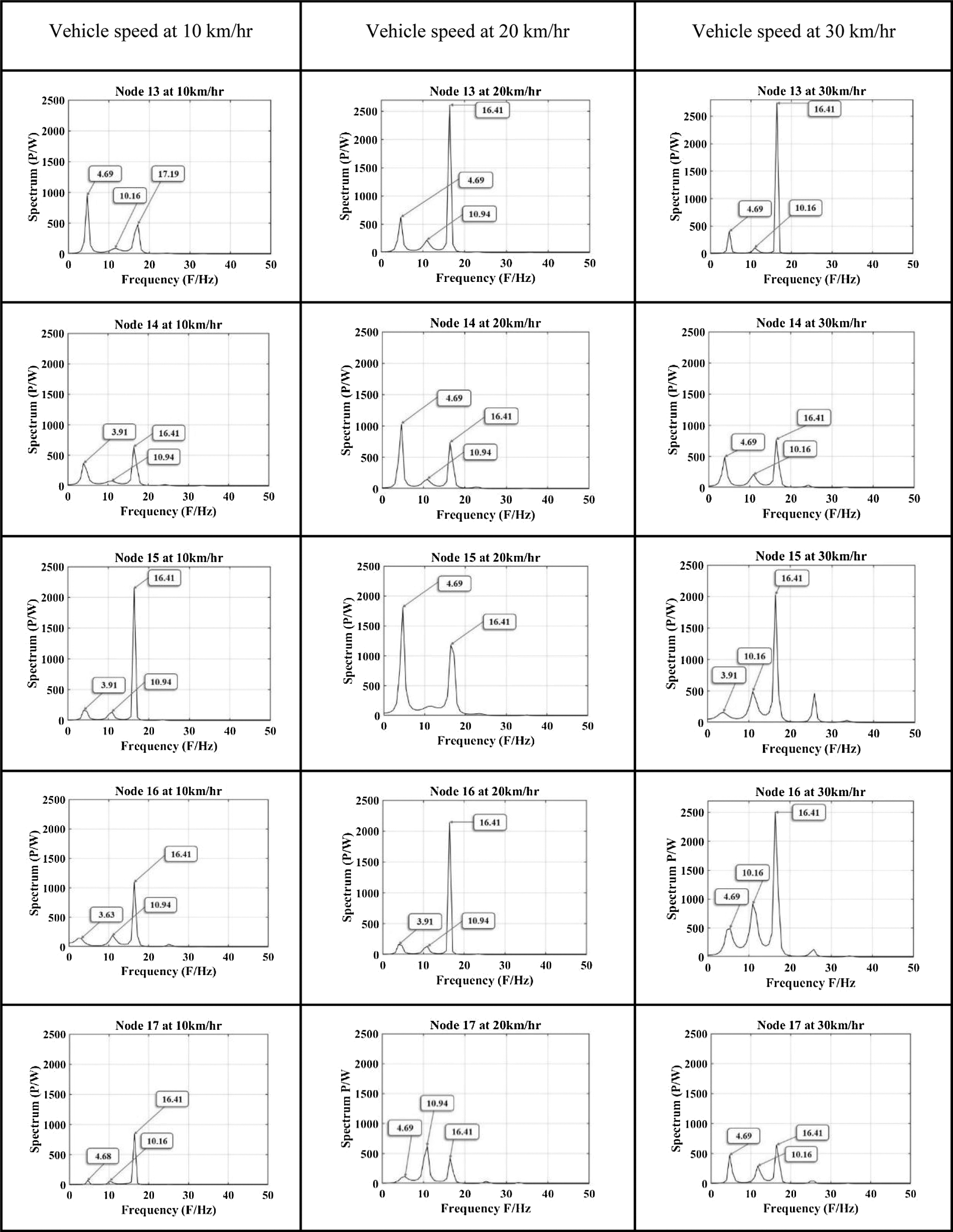
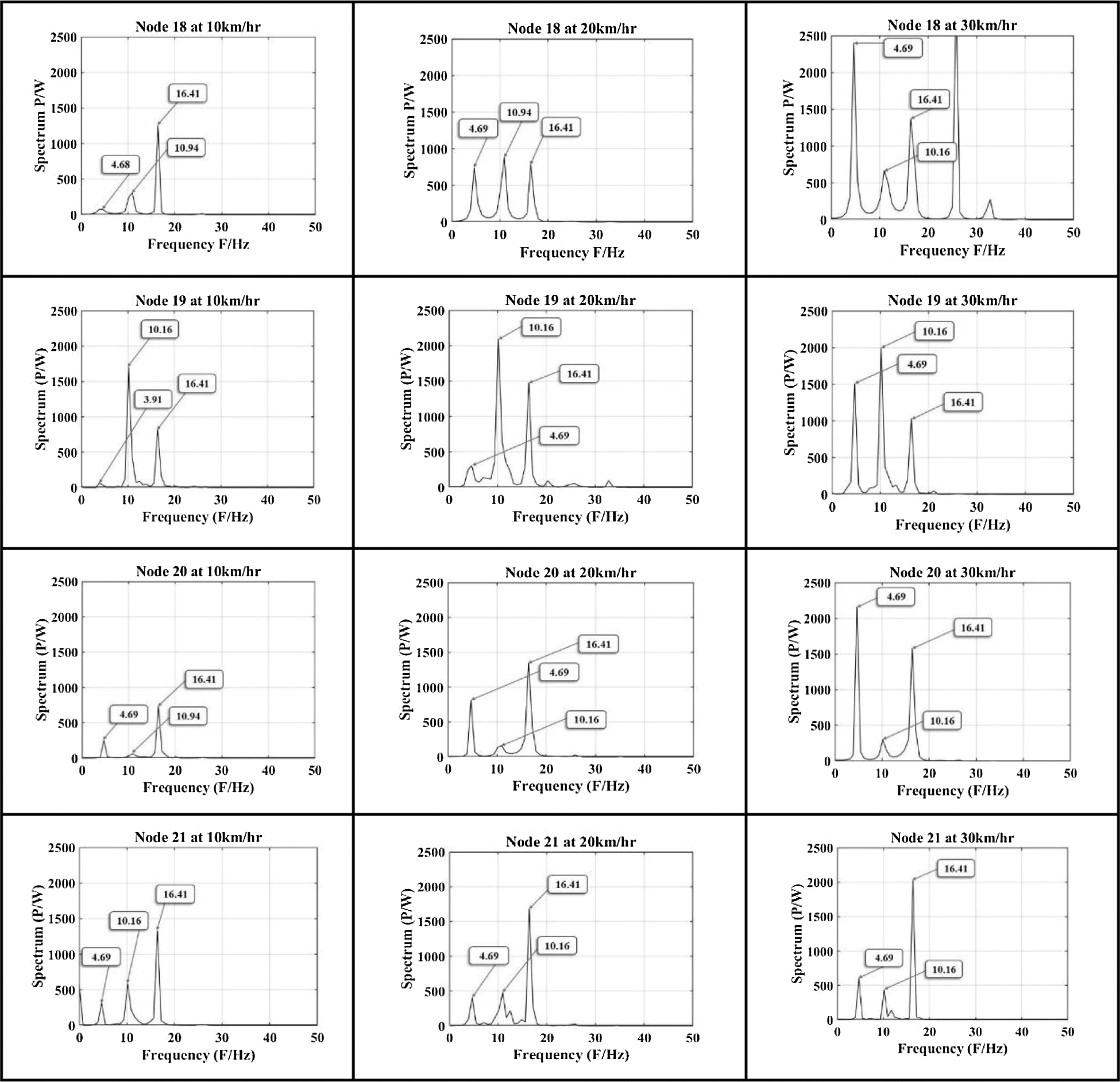
Figure 18: Proposed methodology outcomes for upstream nodes of steel truss bridge
For the upstream nodes at 10 km/hr vehicular speed the 1st modal frequency is obtained at all the nodes. The nodes 13, 14, 20, and 21 showed higher amplitude relatively to the other nodes. The 2nd modal frequency is present at all the nodes. All the nodes showed a low amplitude for 2nd modal frequency except nodes 19 and 21. The 3rd modal frequency is present at all the nodes. The nodes 15, 16, 17, 18, and 21 showed higher amplitude relatively to the other nodes. At 20 km/hr vehicular speed the 1st modal frequency is present at all the nodes. The nodes 16, 17, and 19 showed a low amplitude for 1st modal frequency relatively to the other nodes. The 2nd modal frequency is present at all the nodes except node 15 respectively. The nodes 17, 18, 19, and 21 showed a high amplitude for 2nd modal frequency relatively to the other nodes. At 30 km/hr the 1st modal frequency is present at all the nodes. The nodes 18, 19, 20, and 21 showed a high amplitude relatively to the other nodes. The 2nd modal frequency is present at all the nodes. The nodes 15, 16, 18, and 19 showed higher amplitude relatively to the other nodes. The 3rd modal frequency is present at all the nodes. The nodes 14, 17, and 19 showed low amplitude relatively to the other nodes.
It is observed in the present study that the adopted method provides better denoised outcome of frequencies present in the recorded vibration response signals from the bridge than statistical techniques, and S-transform. The improved resolution of frequency component makes it easy to identify the deficient node through significant variation in modal frequencies. The adopted method of Hilbert transform in combination with spectral kurtosis and bandpass filter is a generalized method which can be applied on any stationary and non-stationary signals collected from any structure (e.g., fault detection in induction motor, turbine, etc.).
In the present study, the novelty is that the proposed methodology uses combined Hilbert transform, spectral kurtosis, bandpass filter and kurtogram for the selection of window length for a high-resolution frequency response which is utilized to unveil the irregularity in the steel truss bridge structure using various speeds of vehicle. The limitation of study is that only first three modal frequencies are obtained from the experimentally measured vibration response data for all the nodes of the bridge. The higher nodes are not able to be extracted accurately and they showed uncertain behaviour with low amplitude. It is observed from the analytical model analysis that the modal load participation factor ratios for first three modes are 96.26%, 93.35%, 91.58%, respectively. The first three modes have shown dominant behaviour to analyze the dynamic behaviour of the bridge structure. The deviation of experimentally obtained modal frequencies w.r.t analytical frequencies shows discrepancies in behaviour of bridge structure. The nodes with increased flexibility and reduced stiffness were identified with the indication of low or missing modal frequency at all three vehicular speeds. The structural deficiency in joining members at the particular nodes can cause peculiarity in nodes behavior. The healthy nodes exhibit modal frequencies in vicinity of analytically obtained modal frequencies of bridge.
• Statistical analysis features, i.e., Crest factor, kurtosis, Impulse Factor, and Peak-to-Peak feature lack confidence for determining the particular behavior as the pattern for a large number of nodes is not obtained with clarity. The kurtosis gives the best pattern among all the statistical features as the speed of the vehicle increases. The kurtosis feature showed a significant irregular rise in amplitude at nodes having structural flexibility deficiencies.
• In the time-frequency domain, the S-transform showed better resolution of modal frequencies plots due to its scalable window and cross-term issue elimination. The unwanted frequencies are obtained in the S-transform plots and require further denoising of the signal to eliminate the noise from vibration signals. The mode value of the obtained frequencies is observed to be the closest to analytical frequency for both downstream and upstream nodes at all vehicular speeds.
• The proposed methodology utilized Hilbert transform, spectral kurtosis, and bandpass filter in combination to extract the hidden dynamic modal information with high resolution. The methodology is performed to obtain the enhanced amplitude modulated signal as compared to the outcomes of statistical features, and S-transform methods. The elimination of the noise is significantly observed with the application of Hilbert envelope analysis and bandpass filtering. The variation in obtained distinct modal frequencies is used to obtain the deficient nodes present in the steel truss bridge.
Acknowledgement: The authors would like to thank the Himachal Pradesh Public Works Department, Government of Himachal Pradesh, India for allowing the National Institute of Technology, Hamirpur to conduct the experiment on the steel truss bridge in the state. The authors also thank Dr. Suresh Kumar Walia for providing necessary experimental data for further signal processing.
Funding Statement: The authors received no specific funding for this study.
Conflicts of Interest: The authors declare that there is no conflict of interest in the context of the publication of this manuscript. In addition, the authors have carefully observed the ethical issues of plagiarism, misconduct, data falsification, or any misconduct while developing the article.
1. Amezquita-Sanchez, J. P., Adeli, H. (2016). Signal processing techniques for vibration-based health monitoring of smart structures. Archives of Computational Methods in Engineering, 23(1), 1–15. DOI 10.1007/s11831-014-9135-7. [Google Scholar] [CrossRef]
2. Tang, Z., Wei, T., Ma, Y., Chen, L. (2019). Residual strength of steel structures after fire events considering material damages. Arabian Journal for Science and Engineering, 44(5), 5075–5088. DOI 10.1007/s13369-018-03711-8. [Google Scholar] [CrossRef]
3. Xu, Y. L., Zhang, C. D., Zhan, S., Spencer, B. F. (2018). Multi-level damage identification of a bridge structure: A combined numerical and experimental investigation. Engineering Structures, 156(3), 53–67. DOI 10.1016/j.engstruct.2017.11.014. [Google Scholar] [CrossRef]
4. Liu, Z. (2009). Reconnaissance and preliminary observations of bridge damage in the great wenchuan earthquake, China case studies: Five Near-fault. Structural Engineering International, 19(3), 277–282. DOI 10.2749/101686609788957883. [Google Scholar] [CrossRef]
5. Prendergast, L. J., Limongelli, M. P., Ademovic, N., Anžlin, A., Gavin, K. et al. (2018). Structural health monitoring for performance assessment of bridges under flooding and seismic actions. Structural Engineering International, 28(3), 296–307. DOI 10.1080/10168664.2018.1472534. [Google Scholar] [CrossRef]
6. Biezma, M. V., Schanack, F. (2007). Collapse of steel bridges. Journal of Performance of Constructed Facilities, 21(5), 398–405. DOI 10.1061/(ASCE)0887-3828(2007). [Google Scholar] [CrossRef]
7. Wang, C. S., Wang, Q., Xu, Y. (2013). Fatigue evaluation of a strengthened steel truss bridge. Structural Engineering International, 23(4), 443–449. DOI 10.2749/101686613X13627347100112. [Google Scholar] [CrossRef]
8. Macho, M., Ryjacek, P., Matos, J. (2019). Fatigue life analysis of steel riveted rail bridges affected by corrosion. Structural Engineering International, 29(4), 551–562. DOI 10.1080/10168664.2019.1612315. [Google Scholar] [CrossRef]
9. Vonk, E. (2019). Innovative approaches to steel bridge repair and strengthening around the globe. Structural Engineering International, 29(4), 1–5. DOI 10.1080/10168664.2019.1649099. [Google Scholar] [CrossRef]
10. Kot, P., Muradov, M., Gkantou, M., Kamaris, G. S., Hashim, K. et al. (2021). Recent advancements in non-destructive testing techniques for structural health monitoring. Applied Sciences, 11(6), 1–20. DOI 10.3390/app11062750. [Google Scholar] [CrossRef]
11. Wang, X., Chang, C. C., Fan, L. (2001). Non-destructive damage detection of bridges: A status review. Advances in Structural Engineering, 4(2), 75–91. DOI 10.1260/1369433011502372. [Google Scholar] [CrossRef]
12. Li, J., Hao, H. (2016). Health monitoring of joint conditions in steel truss bridges with relative displacement sensors. Measurement, 88(6), 360–371. DOI 10.1016/j.measurement.2015.12.009. [Google Scholar] [CrossRef]
13. Sony, S., Laventure, S., Sadhu, A. (2019). A literature review of next-generation smart sensing technology in structural health monitoring. Struct Control Health Monitoring, 26(3), 1–22. DOI 10.1002/stc.2321. [Google Scholar] [CrossRef]
14. Li, J., Deng, J., Xie, W. (2015). Damage detection with streamlined structural health monitoring data. Sensors, 15(4), 8832–8851. DOI 10.3390/s150408832. [Google Scholar] [CrossRef]
15. Dhamande, L. S., Chaudhari, M. B. (2018). Compound gear-bearing fault feature extraction using statistical features based on time-frequency method. Measurement, 125(4), 63–77. DOI 10.1016/j.measurement.2018.04.059. [Google Scholar] [CrossRef]
16. Zhang, Q. W. (2007). Statistical damage identification for bridges using ambient vibration data. Computers & structures, 85(7–8), 476–485. DOI 10.1016/j.compstruc.2006.08.071. [Google Scholar] [CrossRef]
17. Hui, K. H., Ooi, C. S., Lim, M. H., Leong, M. S., Al-Obaidi, S. M. (2017). An improved wrapper-based feature selection method for machinery fault diagnosis. PLoS One, 12(12), 1–10. DOI 10.1371/journal.pone.0189143. [Google Scholar] [CrossRef]
18. Lee, E. T., Eun, H. C. (2016). Structural damage detection by power spectral density estimation using output-only measurement. Shock and Vibration, 2016(1), 1–13. DOI 10.1155/2016/8761249. [Google Scholar] [CrossRef]
19. Pan, H., Azimi, M., Yan, F., Lin, Z. (2018). Time-frequency-based data-driven structural diagnosis and damage detection for cable-stayed bridges. Journal of Bridge Engineering, 23(6), 1–22. DOI 10.1061/(ASCE)BE.1943-5592.0001199. [Google Scholar] [CrossRef]
20. Catbas, F. N., Gul, M., Burkett, J. L. (2007). Damage assessment using flexibility and flexibility-based curvature for structural health monitoring. Smart Material Structures, 17(1), 1–12. DOI 10.1088/0964-1726/17/01/015024. [Google Scholar] [CrossRef]
21. Ben, J., Benbouzid, M., Bechhoefer, E. (2016). The use of SESK as a trend parameter for localized bearing fault diagnosis in induction machines. ISA Transactions, 2016(1), 1–12. DOI 10.1016/j.isatra.2016.02.019. [Google Scholar] [CrossRef]
22. Lee, J., Kim, D., Shin, Y. (2018). Hyperbolic localization of incipient tip vortex cavitation in marine propeller using spectral kurtosis. Mechanical Systems and Signal Processing, (9), 442–457. DOI 10.1016/j.ymssp.2018.03.026. [Google Scholar] [CrossRef]
23. Elforjani, M., Bechhoefer, E. (2018). Analysis of extremely modulated faulty wind turbine data. Renewable Energy, 127(11), 258–268. DOI 10.1016/j.renene.2018.04.014. [Google Scholar] [CrossRef]
24. Walia, S. K., Patel, R. K., Vinayak, H. K., Parti, R. (2013). Joint discrepancy evaluation of an existing steel bridge using time-frequency and wavelet-based approach. International Journal of Advanced Structural Engineering, 5(1), 1–9. DOI 10.1186/2008-6695-5-25. [Google Scholar] [CrossRef]
25. Walia, S. K., Vinayak, H. K., Kumar, A., Parti, R. (2012). Nodal disparity in opposite trusses of a steel bridge: A case study. Journal of Civil Structural Health Monitoring, 2(3–4), 175–185. DOI 10.1007/s13349-012-0021-4. [Google Scholar] [CrossRef]
26. Bearing, L. S., Caesarendra, W. (2015). A review of feature extraction methods in vibration-based condition monitoring and its application for degradation trend estimation of low-speed slew bearing. Machines, 5(4), 1–28. DOI 10.3390/machines5040021. [Google Scholar] [CrossRef]
27. Jin, Z., Li, G., Pei, S., Liu, H. (2017). Vehicle-induced random vibration of railway bridges: A spectral approach. International Journal of Rail Transportation, 5(4), 1–22. DOI 10.1080/23248378.2017.1338538. [Google Scholar] [CrossRef]
28. Xiao, F., Chen, G. S., Hulsey, J. L., Zatar, W. (2017). Characterization of non-stationary properties of vehicle-bridge response for structural health monitoring. Advances in Mechanical Engineering, 9(5), 1–6. DOI 10.1177/1687814017699141. [Google Scholar] [CrossRef]
29. Leonowicz, Z., Lobos, T., Wozniak, K. (2009). Analysis of non-stationary electric signals using the S-transform. COMPEL-The International Journal for Computation and Mathematics in Electrical and Electronic Engineering, 28(1), 204–210. DOI 10.1108/03321640910918995. [Google Scholar] [CrossRef]
30. Neild, S. A., McFadden, P. D., Williams, M. S. (2003). A review of time-frequency methods for structural vibration analysis. Engineering Structures, 25(6), 713–728. [Google Scholar]
31. Zhu, X., Cao, M., Ostachowicz, W., Xu, W. (2019). Damage identification in bridges by processing dynamic responses to moving loads: Features and evaluation. Sensors, 19(3), 463. DOI 10.3390/s19030463. [Google Scholar] [CrossRef]
32. Nagarajaiah, S., Basu, B. (2009). Output only modal identification and structural damage detection using time frequency & wavelet techniques. Earthquake Engineering and Engineering Vibration, 8(4), 583–605. DOI 10.1007/s11803-009-9120-6. [Google Scholar] [CrossRef]
33. Lokhande, A. (2017). A survey on s-transform. IOSR Journal of Electrical and Electronics Engineering, 2(17018), 35–39. https://pdfs.semanticscholar.org/79cc/23f544b66370b408db5bcfddf70393bc6a00.pdf?_ga=2.139988851.1386125652.1590384062-279103949.1572505588. [Google Scholar]
34. Assous, S., Boashash, B. (2012). Evaluation of the modified S-transform for time-frequency synchrony analysis and source localisation. Journal on Advances in Signal Processing, 2012(1), 1–18. DOI 10.1186/1687-6180-2012-49. [Google Scholar] [CrossRef]
35. Kunwar, A., Jha, R., Whelan, M., Janoyan, K. (2013). Damage detection in an experimental bridge model using Hilbert-Huang transform of transient vibrations. Structural Control and Health Monitoring, 20(1), 1–15. DOI 10.1002/stc.466. [Google Scholar] [CrossRef]
36. Sabbaghian-Bidgoli, F., Poshtan, J. (2018). Fault detection of broken rotor bar using an improved form of Hilbert-Huang Transform. Fluctuation and Noise Letters, 17(2), 1–22. DOI 10.1142/S0219477518500128. [Google Scholar] [CrossRef]
37. Liu, H., Wang, X., Lu, C. (2014). Rolling bearing fault diagnosis under variable conditions using Hilbert-Huang transform and singular value decomposition. Mathematical Problems in Engineering, 1–10, DOI 10.1155/2014/765621. [Google Scholar] [CrossRef]
38. Agrawal, S., Mohanty, S. R., Agarwal, V. (2015). Bearing fault detection using Hilbert and high frequency resolution techniques. IETE Journal of Research, 61(2), 99–108. DOI 10.1080/03772063.2015.1009398. [Google Scholar] [CrossRef]
39. Chiang, W. L., Chiou, D. J., Chen, C. W., Tang, J. P., Hsu, W. K. et al. (2010). Detecting the sensitivity of structural damage based on the Hilbert-Huang transform approach. Engineering Computations, 27(7), 1–20. DOI 10.1108/02644401011073665. [Google Scholar] [CrossRef]
40. Hsu, W. K., Chiou, D. J., Chen, C. W., Liu, M. Y., Chiang, W. L. et al. (2013). Sensitivity of initial damage detection for steel structures using the Hilbert-Huang transform method. Journal of Vibration and Control, 19(6), 857–878. DOI 10.1177/1077546311434794. [Google Scholar] [CrossRef]
41. Feng, G. J., Gu, J., Zhen, D., Aliwan, M., Gu, F. S. et al. (2015). Implementation of envelope analysis on a wireless condition monitoring system for bearing fault diagnosis. International Journal of Automation and Computing, 12(1), 14–24. DOI 10.1007/s11633-014-0862-x. [Google Scholar] [CrossRef]
42. Yang, J. N., Lei, Y., Lin, S., Huang, N. (2004). Hilbert-Huang based approach for structural damage detection. Journal of engineering mechanics, 130(1), 85–95. DOI 10.1061/(ASCE)0733-9399(2004)130:. [Google Scholar] [CrossRef]
43. De Carlo, L. T. (1997). On the meaning and use of kurtosis. Psychological Methods, 2(3), 292. [Google Scholar]
44. Feldman, M. (2011). Hilbert transform in vibration analysis. Mechanical Systems and Signal Processing, 25(3), 735–802. DOI 10.1016/j.ymssp.2010.07.018. [Google Scholar] [CrossRef]
45. Lei, Y., Lin, J., He, Z., Zi, Y. (2011). Application of an improved kurtogram method for fault diagnosis of rolling element bearings. Mechanical Systems and Signal Processing, 25(5), 1738–1749. DOI 10.1016/j.ymssp.2010.12.011. [Google Scholar] [CrossRef]
46. Combet, F. Ã., Gelman, L. (2009). Optimal filtering of gear signals for early damage detection based on the spectral kurtosis. Mechanical Systems and Signal Processing, 23(3), 652–668. DOI 10.1016/j.ymssp.2008.08.002. [Google Scholar] [CrossRef]
47. Antoni, J., Randall, R. B. (2006). The spectral kurtosis: Application to the vibratory surveillance and diagnostics of rotating machines. Mechanical Systems and Signal Processing, 20(2), 308–331. DOI 10.1016/j.ymssp.2004.09.002. [Google Scholar] [CrossRef]
48. Antoni, J. (2007). Fast computation of the kurtogram for the detection of transient faults. Mechanical Systems and Signal Processing, 21(1), 108–124. DOI 10.1016/j.ymssp.2005. [Google Scholar] [CrossRef]
 | This work is licensed under a Creative Commons Attribution 4.0 International License, which permits unrestricted use, distribution, and reproduction in any medium, provided the original work is properly cited. |