Structural Durability & Health Monitoring

DOI: 10.32604/sdhm.2021.012751

ARTICLE

Comparative Analysis of Wavelet Transform for Time-Frequency Analysis and Transient Localization in Structural Health Monitoring

Ahmed Silik1,2, Mohammad Noori3,*, Wael A. Altabey1,4, Ramin Ghiasi1 and Zhishen Wu1

1International Institute for Urban Systems Engineering (IIUSE), Southeast University, Nanjing, 210096, China
2Department of Civil Engineering, Nyala University, Nyala, Sudan
3Department of Mechanical Engineering, California Polytechnic State University, San Luis Obispo, CA 93405, USA
4Department of Mechanical Engineering, Faculty of Engineering, Alexandria University, Alexandria, 21544, Egypt
*Corresponding Author: Mohammad Noori. Email: mnoori52@yahoo.com
Received: 11 July 2020; Accepted: 09 September 2020

1  Introduction

Structures may collapse due to destructive man-made or natural hazards and events. Even if a structure can resist, and survive the destructive wave propagation during a disastrous event and does not necessarily collapse, the induced vibrations may likely cause an unknown level of damage. Therefore, a structural evaluation is necessary to diagnose the health of the structure. The critical stage in any structural evaluation is to process the measured responses [1]. At this point, the measured signals are analyzed to extract specific characteristics, such as modal parameters, or to directly create a model that matches the data, as in the case of system identification. In SHM applications, signal processing techniques can address various issues, tasks, and analysis methods, such as (i) Data acquisition and measurements, (ii) Data pre-processing, (iii) Signal feature analysis, (iv) Pattern recognition and machine learning [2,3] (v) Reliability analysis, (vi) Uncertainties, and (vii) Data fusion [4]. Most strategies in SHM depend on various measurements such as vibration acceleration [5,6], displacement, strain, or temperature, through signal processing, and electrostatic signal [7,8]. Thus, signal processing is the main component in SHM and a critical step toward an integrated intelligent system design [9,10]. Wavelet analysis, among other signal analysis tools, has proven to be a robust technique for non-stationary signal analysis due to its ability to localize in time and frequency domains [11,12]. An attractive aspect of wavelet transform is that it can be dilated across various widths to capture different frequencies. Multiple studies have used various WT in other applications to analyze various real-world signals to detect structural damage [9]. A wide range of wavelet functions have been reported in the literature; however, to the best of the authors’ knowledge, very limited discussions or strategies have been presented in the literature on how to choose the best wavelet for a specific task. The most commonly used approach has been to select a wavelet matched to the analyzed signal and subsequently try several wavelets via this approach. The wavelet function must be square-integrable and have no energy at zero frequency (bandpass). For an overview of wavelets and their applications, please see [13,14].

Both discrete WT and continuous WT have been used for vibration monitoring. However, the main issue in using WT is how to choose the wavelet parameters for a specific task. Selecting the right wavelet is an essential requirement in the wavelet analysis of a given signal. An appropriate mother wavelet displays the wavelet ability in de-noising, signal retaining, and feature extraction and improves the de-noised signal’s frequency spectrum [15–17].

Over the last two decades various studies have been conducted using multiple quantitative measures, that are essential, to select optimum wavelets; such as correlation index, variance, maximum energy, and entropy [18–21]. However, in some literature associated with this topic, it is erroneously assumed that any wavelet function and type is valid for any data and any application. Currently, there is no general guidelines, or universally applicable criterion, for the wavelet choice that caters to all applications. Despite the lack of any widely accepted set of rules, various wavelets have been used for damage detection, and their efficiency has been evaluated [22–25]. One criticism about using wavelet analyses in the structural application has been the random and ah-hoc approach used for selecting the mother wavelet. Most studies reported in the literature have focused on the similarity between signal and mother wavelet, although the similarity is not the proper function for all wavelet-based signal processing applications.

Overall, a structure’s dynamic responses are due to disturbances caused by operational and environmental conditions. In general, high-frequency events often have a shorter duration, while low-frequency events have a more extended period. Thus, a robust time-frequency technique to analyze how the frequency content of signal changes over time is necessary.

In summary, since WT application for the response analysis of different structures has been limited to using theoretical and ad-hoc measures for choosing the right type and optimum wavelets, researchers, have not introduced any explicit criteria for selecting the appropriate type and mother wavelets. Therefore, the main goal of the research presented in this paper is to choose the proper wavelet type and mother wavelet for time-frequency analysis of structural dynamic responses. Subsequently, the acceleration responses and their wavelet scalograms are used to show the most informative time-frequency regions to detect the location and the occurrence time of the damage qualitatively. The proposed strategy considers wavelet type, data characteristics, and objective measures to select the proper wavelet type suitable for different structural damage detection applications. Finally, the scalogram’s informative time-frequency regions are examined to analyze the wavelet coefficient variation and to show how the frequency content of a signal changes over time, in order to detect the transient events due to damage qualitatively. Although herein, the CWT description is the main focus, the potential advantages of DWT have also been investigated to show the CWT’s ability compared with other types.

This paper is organized as follows. Section 2 shows the variations between continuous and discrete wavelet. Section 3 describes the wavelet choice strategy and guideline. Section 4 describes Time-Frequency Analysis using CWT. Section 5 describes the numerical analysis studies that have been conducted. Finally, Section 6 presents the results, discussions, and conclusions of this study.

2  Continuous vs. Discrete Wavelet Transform

There are various types of wavelet analysis, classified as DWT and CWT [26]. For a successful and effective signal processing analysis using WT, it is necessary to recognize the differences between them. Historically, CWT was developed and introduced in the literature before DWT, and it was mainly used as an alternative for the Fourier transform. CWT is a function of analog filtering, similar to DWT, with low and high-pass filtering at various scales. However, the filtering functions are done on the input in parallel, as a filter bank, with high and low pass functions combined into a single bandpass function. The various scales are understood as neighboring bands in the frequency domain, increasing the bandwidth corresponding to the band center frequency. Thus, CWT is characterized as a constant-Q filter bank. DWT gives an equivalent result, starting with a block of discrete data and carrying out sequential filtering of high and low frequencies. Filtering is repeated at the low-frequency output as in normal DWT and repeated at the low and high-frequency output as in discrete packet transform (PWT) generated from DWT to transmit a signal in a series of steps known as scaling. Each scaling divides the current interval’s frequency space in half, doubling the time interval, hence, preserving a constant time-frequency product.

In contrast, CWT divides the signal into a set of frequency bands of a logarithmic scale, passing it through a series of bandpass filters with a constant Q bandpass filter. Both CWT and DWT are filter banks, although CWT takes a more intuitive form of a physical filter with a transfer function in the time and frequency domains. DWT filters are wisely formulated mathematical models whose transfer functions are recursive. Due to limitations in the DWT specification, all DWT filters have compact support. DWT is limited in time and frequency and has been proven that it cannot be applied through physical filters in the continuous-time domain. Being physically achievable, CWT cannot achieve ideal compact support. Instead, similar to the way elliptical filters, such as Chebyshev and Butterworth, are generated, CWT functions are created to achieve maximum compactness according to specific criteria. Both CWT and DWT are decimated, and non-decimated versions, and the significant difference between them is how the scale parameter is discretized. The scale values define to which degree the wavelet can be stretched or compressed. The low-scale values compress the wavelet and correlate better with the high-frequency content of the signal. The low-scale components of CWT represent the accurate fine-scale characteristics of the analyzed signal. High scale values stretch the wavelet function and better correlate with the low-frequency components. The high-scale components of CWT represent the rough coarse-scale characteristics of the analyzed signal. For the detailed application of various types of wavelets in civil engineering, readers can refer to [27].

2.1 Wavelet Discretization

Concerning wavelet implementation, DWT and CWT vary according to how the set of scales or frequencies (wavelet width) are selected. CWT discretizes finer scales than DWT, however, DWT is easier to implement. In CWT, exponential scales are usually used with a base smaller than 2 to obtain different scales; for instance, 2j/v where v is an integer > 1 and is the number of voices per octave, and   j = 1, 2, 3….The discretized wavelet for CWT is expressed as:

ψj,k(t)=12j/υψ(t−k2j/υ) (1)

where 2j/υ=s,ak=τ . The typical values for υ are 10, 12, 14, 16, and 32. The larger the υ , the more accurate the discretization of the scale s will be. However, this increases the computation cost since CWT is computed for each scale. CWT correlates a signal with the following scaled-shifted version base wavelet ψ (t):

ψs,τ(t)=1sψ(t−τs) (2)

If ψ(t) is centered at t =0 with time support [–T/2, T/2], the ψs,τ(t) is centered at t = u with time support [–sT/2+u, sT/2+u]. CWT shows how closely correlated are the wavelet and analyzed function in the time interval, which is defined by the wavelet’s support. Data is broken down into varied base wavelet and is presented as an integral of scaled and shifted wavelets. The coefficients are represented by two-dimensional as:

Ws,τ=1s∫∞−∞⁡x(t).ψ∗(t−τs)dt (3)

By changing the scaling s, we can see how the wavelet corresponds to the signal from one scale to the next, whereas changing the translation t from ψ (t) shows how the nature of the signal changes with time. In the DWT, the scale s is discretized to integer powers of two, 2j, where j = 1, 2, 3..., so that the number of voices per octave is always 1. This is a much coarser scale sampling than the one for CWT. In decimated DWT, the shift is relative to the scale. On the scale, 2j, you move by 2jm. In non-decimated DWT, the scale s is restricted to powers of two, but the translation m is an integer as in the CWT. The discretized wavelet for the DWT is expressed as:

ψj,m(t)=12jψ(12j(n−2jm)) (4)

The discretized wavelet for the non-decimated DWT is defined as:

ψj,m(t)=12jΨ(n−m2j) (5)

It should be noted that the decimated and non-decimated DWT vary in how they discretize the shift parameter. The decimated DWT is translated by 2jm while non-decimated DWT by integer shifts m. It should be remembered that the physical interpretation of the scales for DWT and CWT requires the integration of the signal sampling rate if it is not equal to one. For instance, suppose you use CWT and set your base to s0 = 21/12. In order to assign physical significance to this scale, it should be multiplied by the sampling step Δt as s0j.Δt , so a scale vector covering roughly four octaves with Δt where j = 1, 2…48. For DWT, the base scale is always 2. These variances in the scale and shift discretization approaches have cons and pros for both WT and determine where the one type can provide excellent results. The DWT is expressed as:

Wj,k=2(−j/2)∑n⁡x(t)ψ(2−jt−k) (6)

DWT provides a sparse representation, and the critical characteristics of signals are taken by a subset of the DWT coefficients, which is smaller than the analyzed signal. Thus, the signal is compressed. The coefficient number is the same as the original signal, but most coefficients can be close to zero. So, you can often eliminate these coefficients though de-noising the signal. Using CWT, from N data samples, an M by N matrix of coefficients is obtained, where M is the scale number. CWT is a redundant conversion but has the same time resolution as the original data in each frequency band. There is an overlap between wavelets at each scale and the scales. The computing resources and time needed to perform CWT analysis and store the coefficients are more extensive than DWT. A non-decimated WT is also redundant, but the redundancy coefficient is usually much lower than the one for CWT because the scale parameter is not discretized so finely. For the non-decimated DWT, from N samples, an L+1-by-N matrix of coefficients can be obtained, where L is the decomposition level. The DWT discretization ensures orthonormal transform, which is useful in multiresolution analysis and de-noising beside others. Neither the non-decimated DWT nor the CWT is orthonormal transforms. Due to downsampling, DWT is not shift-invariant, but CWT and non-decimated DWT are. In DWT, the wavelet expression is not required because the filters are sufficient, while in the CWT, those expressions are needed. The non-decimated DWT offers a redundant representation but not similar to CWT. Thus, the application is influenced by wavelet choice and which type of wavelet to be used.

2.2 Wavelet Application

For wavelet application in different structures, CWT is the ideal candidate for time-frequency analysis [28]. For that reason, it is usually selected in most tasks, for instance, to localize the transients in the signal or for other applications such as characterizing oscillatory behavior, singular detection, detecting discontinuities in higher derivatives, identifying breakdown points, and self-similarity [29]. Multiresolution analysis through DWT has good energy compactification and sparse representation. The orthogonal DWT can result in a perfect recovered signal, while CWT often can not provide a perfect recovered signal because it is a much less stable numerical operation. However, to localize transients or characterize oscillatory behavior, CWT gives a better result compared with DWT [30], and the plots obtained with CWT are easier to interpret than those obtained with the DWT [31]. Based on the above discussion, both continuous and multiresolution analysis must be used to analyze dynamic measurements in structural analysis applications. Fig. 1 shows the comparison between CWT and DWT absolute coefficients. CWT shows better results than DWT due to finer scales, resulting in higher-fidelity signal analysis. Fig. 2 shows the type of wavelet, wavelet application, and challenges in using wavelet analysis for non-stationary structural dynamic measurements.

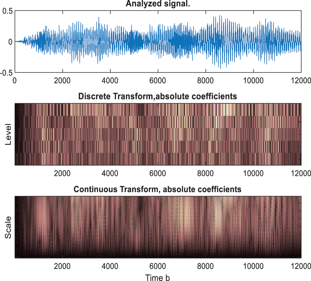
Figure 1: Comparison between CWT and DWT absolute coefficients

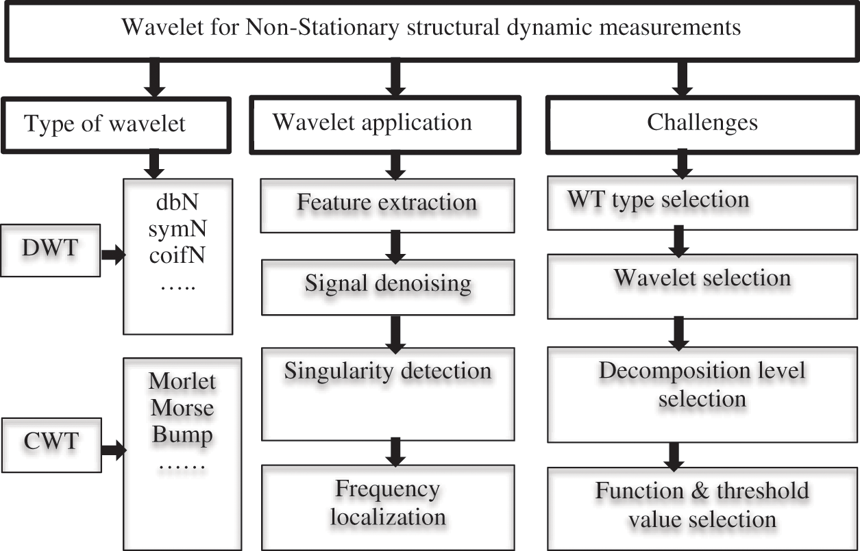
Figure 2: Type of wavelet, wavelet application and challenges in using wavelet analysis for non-stationary structural dynamic measurements

2.3 Wavelet Analysis in Damage Detection

Measured responses can be treated as spatially distributed input signals, and their wavelet transform can be computed [32]. CWT is a robust tool for analyzing non-stationary data in the time-frequency domain and somewhat differing from the short Fourier transform (STFT) that allows precise localization on the frequency components’ time axis of the analyzed signals. It allows for accurate scale plane decomposition, but the scaled translated versions of the base wavelet do not have orthogonality characteristics. Whenever this characteristic is essential, it may be useful to resort to orthogonal bases. As for application, CWT is the ideal candidate for damage detection based signal analysis due to its finer resolution [22] and is usually chosen in most tasks (e.g., abrupt changes and singularity detection). DWT is of more interest in the context of fast non-redundant transforms so that a continuous scale can be changed to a varying scale limited to dyadic sequence ( s=2j ). This leads to the advantages of DWT which include reduction in computations cost and memory requirements. DWT is mainly suitable for eliminating noise and compressing the signal. However, in the case of determining the damage location in structures, higher scales are required. Thus, the DWT’s applicability for damage detection is limited and has two drawbacks for using in damage detection. The first one is the length of the wavelet coefficient vector decreases by half of its initial size at each scale level j. The second one is the fact that the scale is limited by the dyadic sequence ( s=2j ). Thus, comparing s = 64 and s = 128, there is a large gap in the wavelet resolution, and valuable information may be lost. This shortcoming can be described as trying to find cracks on a wall at night by using only a low-intensity light source, such as a torch. If the light is directed at one part of the wall, then turned off, and subsequently moved to another position, some of the cracks may be lost, or the crack will not be detected. But at least if the light continually moves along the wall, damages can be detected. Thus, the computation time cannot be limited in this case, and the application of the continuous scales is recommended [33]. It has been demonstrated that CWT can show/capture the signal frequency content with finer accuracy and much more details, in contrast to DWT or Fourier analysis. Moreover, CWT also has the same time resolution as the analyzed data in each frequency band. Therefore, CWT is the appropriate candidate for time-frequency analysis and is usually selected in most tasks such as localizing transients in the signal or characterizing oscillatory behavior and singularity detection.

3  Wavelet Selection Guidelines and Criteria

Based on the above discussion, and depending on what we want to do with the dynamic response measurements, as illustrated in Fig. 2, herein are some suggested and basic guidelines for deciding whether to use CWT or DWT. (i) For the sparsest signal representation for de-noising, compression, or signal feature extraction, multiresolution analysis through DWT/PWT is a suitable choice. (ii) For the application that requires a shift-invariant transformation but still needs perfect reconstruction and some computational efficiency measure, non-decimated DWT is a suitable choice. (iii) For detailed time-frequency analysis or accurate signal transient localization, especially for signals in which the instantaneous frequency grows rapidly, CWT is the right choice [21]. Based on these guidelines, CWT is the best choice for our objective. To further quantitatively evaluate various analytic and non-analytic wavelet’s performances, multiple measures based on wavelet energy density distribution and wavelet mutual information have been calculated to assess the best candidate base wavelets. These measures are examined from two varied aspects: (i) Their corresponding wavelet coefficients and (ii) The relationship between the analyzed signal and the analyzed wavelet coefficients. To visualize the percentage energy content for each coefficient, the scalogram and contour plots are used.

3.1 Wavelet Family

Wavelet families vary from one to another because every family has a different trade-off in how compact and smooth the wavelet looks like. This means that a given wavelet family can be chosen such that it fits best with the features we are looking for in our data. Each type has a different shape, compactness, and smoothness and is useful for various purposes. From the practical point of view, both analytic and non-analytic wavelets are used in CWT, and most of them are defined in the frequency domain. Analytic functions are wavelets with one-sided spectra (FT is zero for ω < 0). Following base wavelets are dominantly used in CWT applications and have been especially useful for time-frequency analysis.

Morse wavelet: Generalized Morse wavelet family ψβ, γ (t), is parametrized by an oscillation control parameter β > 0, a shape parameter γ > 0, and order parameter k, that belong to Z ≥ 0, to change time and frequency spread and gives a broad range of forms and characteristics. It is useful for analyzing modulated signals and localized discontinuities [34]. More details are presented in the work of Jonathan et al. [35]. Morse Waveket is defined in the frequency domain as:

ψβγ(ω)=∫−∞∞⁡ψβγ(t)exp⁡(−iωt)dt=U(ω)aβγωβexp(−ωγ) (7)

Morlet wavelet: Morlet wavelet is designed to be a zero-mean function, and it represents a sinusoidal function modulated by a Gaussian function [36,37]. It is a function of infinite duration, but most of the energy is confined to a finite interval [36]. It has equal variance in time and frequency and is suited to detect good time and frequency localized information. This mother wavelet has no scaling function and does not technically satisfy the admissibility condition, except only approximately. However, if α > 5.5, the error can be ignored numerically. It is defined as:

ψ(t)=exp(−β2t2/2)cos(πt) (8)

By dilation with a and translation with b, the Morlet wavelet family can be expressed as:

ψa,b(t)=exp[−β2(t−b)2a2]cos[π(t−b)a] (9)

The real part is defined as:

ψ(t)=(β2π.e−β2t2/2).cos(ωct) (10)

where β is a number of cycles used to control the wavelet shape and balance time and frequency resolution. The Complex Morlet wavelet is defined as:

ψ(t)=1πfbei2πfcte−t2/fb (11)

where fb is a bandwidth parameter that controls the wavelet shape and wc = 2πfc is the central wavelet frequency, which determines the oscillations number of the complex sinusoid inside the symmetric Gaussian envelope. To assure that the above expression is a wavelet (a zero-mean function), it must have an fc > 5. Usually fc = 6 for engineering applications [38], since the wavelet becomes skewed at fc < 5 [39]. The term 1/π4 ensures that the wavelet has unit energy. This wavelet has been successfully used for vibrational signals analysis [40].

Bump wavelet: Bump wavelet is a bandlimited function defined in the frequency domain with parameters μ and σ and window w [41]. It has a broader variance in time and a narrower variance in frequency. Valid values for μ are in the range of (3, 6) and for σ are in the range of (0.1, 1.2). Smaller values of σ give rise to wavelets with superior frequency localization but poorer time localization. Larger values of σ produce a wavelet with better time localization and poorer frequency localization. It can be defined as:

ψ^(sω)=e(1−11−(sω−μ)2ρ2).I[μ−σs,μ+σs] (12)

where I[(μ−σ)/s,(μ+σ)/s] is the indicator function for the interval.

Meyer wavelet: Meyer wavelet is orthogonal and differentiable with unlimited support. It is defined in the frequency domain [42] as:

ψ^(ω)={(2π)−12eiω2.in(π2v(32π|ω|−1))if2π3≤|ω|≤4π3(2π)−12eiω2.cos⁡(π2v(32π|ω|−1))if4π3≤|ω|≤8π30otherwise (13)

This results in scaling functions and wavelets with unlimited support but decays quicker than the sine wavelet.

ν(x):={0ifx<0xif0<x<11ifx>a. (14)

Mexican hat wavelet: Mexican hat wavelet (Ricker wavelet) is proportional to the negative value of the second derivative of a Gaussian function. Most of its energy is within the interval (–5, 5), which is the correct theoretical adequate support. However, adequate support (–8, 8) is used to provide more accurate results [43]. There is no scaling function associated with this wavelet and it has a functional form as:

ψ(t)=23σπ1/4(1−(tσ)2)e−t22σ2 (15)

where σ is the standard deviation that controls the width, and t is an independent variable.

To successfully track the damage-induced changes in the structural dynamic characteristics with time-frequency representation based on CWT, the mother wavelet parameters are selected. Based on the above discussion and the authors’ experience, Morel wavelet number of cycles fc = 6, Morse wavelet shape parameters γ = 3, control parameter β = 60, Mexican hat wavelet support (–8, 8) and Bump wavelet and Meyer wavelet are used as default in Matlab.

3.2 Quantitative Analysis of Continuous Wavelet Transforms

Wavelet Energy Distribution: Wavelet energy distribution with time and frequency is used to recognize the local characteristics and can be used to characterize the signal x (t). Thus, it can be used for choosing the base wavelet. Since discrete sample values represent the data, the amount of the signal energy contained is expressed as:

Ex(i)=∑i=1N⁡|x(i)|2 (16)

The signal energy content can also be acquired from its wavelet components (wt(s, i)) and is expressed as:

Eenergy=∑s⁡∑i⁡|wt(s,i)|2 (17)

This shows that the energy associated with each specific scaling factor s is defined as:

Eenergy(s)=∑i=1N⁡|wt(s,i)|2 (18)

Besides the energy, Shannon Entropy can also be computed using the detail coefficients to express the wavelet energy distribution as:

Eentropy(s)=∑i=1N⁡pi.log2pi (19)

The function that minimizes the entropy represents the best wavelet for transient detection. The appropriate wavelet should maximize the energy and reduce the entropy by combining the entropy and energy. The distribution of relative wavelet energy-entropy ratio is defined as:

R(s)=Eenergy(s)Eentropy(s) (20)

Wavelet mutual information analysis: A wavelet mutual information is a concept that clarifies the relationship between an analyzed wavelet and an analyzed signal. In other words, mutual information is the uncertainty reduction in one variable due to gaining more knowledge about the other. Mutual information basically is a measure of the information contained in random variable x about the random variable y. In the wavelet domain, mutual information quantities can be defined between a wavelet coefficient and its parent coefficients and between a wavelet coefficient and its adjacent wavelet coefficients. This important measure can be found in a way somewhat similar to the classical definition I(x; y) = H(x) – H(x|y) after using Bayes’ rule, where H(·) is the entropy function, which is the uncertainty measure of the variable. The information provided by wavelet signal decomposition is given [44] as:

(f(t).{Ψa,b(t)})=∫−∞+∞⁡∫−∞+∞|CWT(a,b)|2E.cΨ.|a|2.log(E.cΨ.|CWT(a,b)|2∫−∞+∞⁡|CWT(a,b)|2db∫−∞+∞⁡|CWT(a,b)|2daa2)dadb (21)

A joint probability p (x, y); over the scale-translation domain can be defined as:

P(a,b)=|CWT(a,b)|2E.cΨ.|a|2,a≠0 (22)

Thus, this joint density is expressed through the signal scalogram, which visually can provide information on local features hidden in the data [44]. The mutual wavelet information can be derived from the homogeneous wavelet expansion as:

I(f,{Ψ})=∑n∈Z∑m∈Z|wn,m|2Elog2E.|wn,m|2∑m′∈Z|wn,m′|2∑n′∈Z|wn′,m|2 (23)

4  Wavelet Scalogram

Various wavelets have a good localization in time and frequency, which is a desirable characteristic for damage detection in nonlinear structural dynamic systems using non-stationary signals [23]. CWT automatically adjusts the resolution in time and frequency depending on the scale of the activity of interest, expanding or compressing the analysis window. As the wavelet is compressed (a < 1), it provides a high temporal resolution and is well suited for determining the short-term events, such as jumps and transients. As the wavelet is expanded (a > 1), it provides a high spectral resolution and is well suited for determining the long-term events, such as baseline fluctuations. Likewise, knowing the long-term frequency is often more interesting than knowing the exact onset of change since it is gradual. Wavelet scalogram-based CWT is one of the fundamental tools of wavelet-based fault diagnostics [45] and is defined as the wavelet transform modulus square.

S=|wt(s,i)|2,SC=100∗S/sum(S) (24)

The wavelet scalogram measures the signal’s local time-frequency energy density and provides useful information about the structure's behavior over time [46]. The scalogram can be presented in 2D contours with time as the horizontal axis and scale as the vertical axis, and the coefficient given by a gray-scale color. Alternately, the coefficient can be plotted in 3D contours. Its plot represents the percentage of energy for each coefficient. It can reveal previously hidden information about the nature of non-stationary processes. Scalogram is widely used in various vibration signal analysis areas, including de-noising, structural, ground motion analysis, fault diagnosis, damage detection, and many other applications [45,47]. Thus, in this paper, we use a scalogram to carry out a comparative study using different analytic wavelets, including Morlet, Morse, Bump, and non-analytic functions, including real Morlet, Mexican hat, and Meyer wavelets. This comparative analysis is conducted by studying these wavelets’ characteristics in a time-frequency domain to show their ability to simultaneously detect activity at different scales and disclose low-frequency characteristics of data hidden in a time series. Finally, it is used to analyze the variation of wavelet coefficients between damaged and undamaged states and to evaluate the wavelet’s effectiveness. For comparison purposes, the scalogram is normalized by dividing it by the square root of the number of times.

5  Numerical Simulations

In order to realize structural damage identification using the signal-based technique, it is essential to obtain, in advance, the structural dynamic response with varied damage scenarios. Since it is almost impossible to analyze a physical structure with various types and extents of damages, a computational model is considered for analyzing multiple damage scenarios.

5.1 Structural Model

A simulated 3D 3-story moment resisting concrete frame building with a total height of 9 m, as illustrated in Fig. 3a, is considered. The frame is modeled as a spring-mass-damper discrete model shown in Fig. 3b. All story masses have the same value of 300 kg, and the initial spring stiffness of each column is 100 kN/m. The damping is assumed to be a Rayleigh damping related to the stiffness with a factor of 0.05.

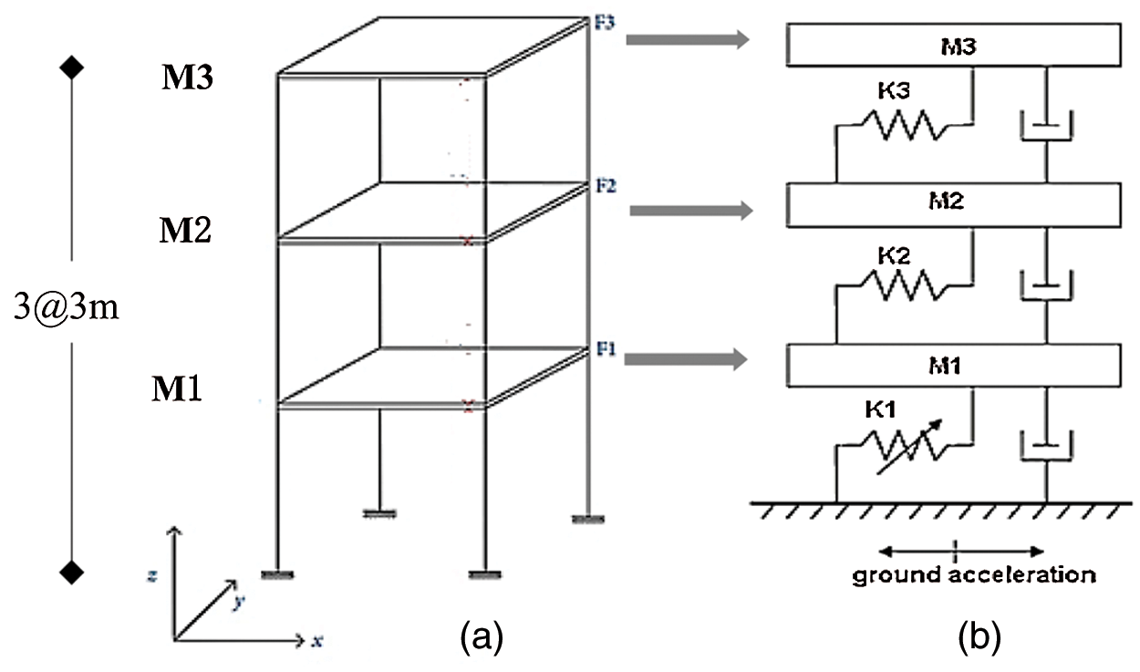
Figure 3: Analytical model. (a) Model of a three-story frame structure (b) Spring-mass-damper model

5.2 Dynamic Excitation Loads

Random excitation load is modeled as a discrete Gaussian white noise process with a zero mean, and a root mean square value of 0.5 m/s2. The dynamic load is generated using the “rand” function in Matlab, which can yield random numbers between zero and one. The dynamic loads are applied to the structure base as a ground acceleration, and the responses are drawn out from a point at the top right of the structure.

5.3 Damage Pattern Database Simulation

Damage levels can be numerically simulated by changing the properties of the baseline model of the structure, i.e., EI, of the damaged components. This simulation is one of the commonly used damage detection techniques in SHM. For illustration purposes, it is assumed that the sample structure has experienced a 40% stiffness reduction on the first floor, while the stiffness on the other floors remains unchanged. Two sets of known damage cases, including the baseline condition, were chosen as the possible structural damage conditions for the sample structure. The analytical model’s dynamic acceleration responses with various possible damages were obtained by numerical simulation (Newmark-method) at the floor level of each story under horizontal ground acceleration at the base. The structure is analyzed under simulated dynamic load using the Matlab version 2020a. To simulate the limitations associated with data encountered in the real field, the simulated data is contaminated with additive white noise to evaluate the robustness of the proposed technique in the presence of the measurement noise. The additive noise level is characterized by the signal to noise ratio (SNR), which is the ratio of the magnitude of noise-free signal (x) to the magnitude of noise (n). Herein, SNR is expressed in terms of the standard deviation, SNR=σu/σn ; where σu is the noise-free signal standard deviation and σn is the noise standard deviation such that the observed signal is x^ = x + n. All sets of simulated acceleration responses were transformed by FFT.

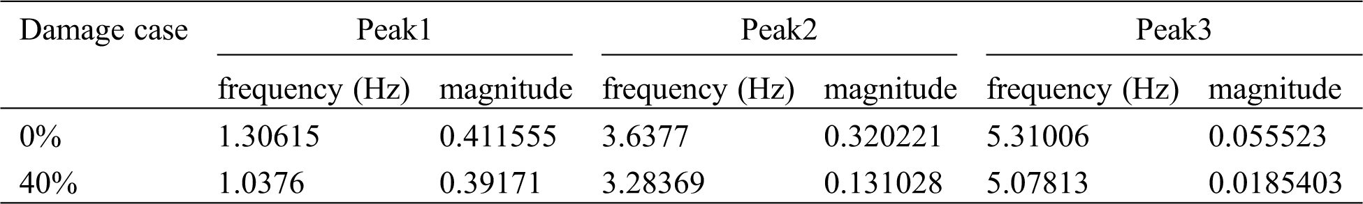
Figs. 4 and 5 reveal the acceleration responses from damaged and undamaged status in various stories, respectively, with their corresponding spectra. It is shown that each signal contains three components within the first 10 seconds, and there are slight ripples; they may arise due to sudden changes from one frequency component to another. Also, the amplitudes of lower frequency components are higher than those of the higher frequency components. This is because lower frequencies last longer than the higher frequency components. Tab. 1 shows the frequencies and magnitudes corresponding to the three peaks of signal spectrums of floor1. It shows that due to different damage cases, there is a reduction in amplitude values and frequency values of spectra of damage state compared with spectra of undamaged condition.

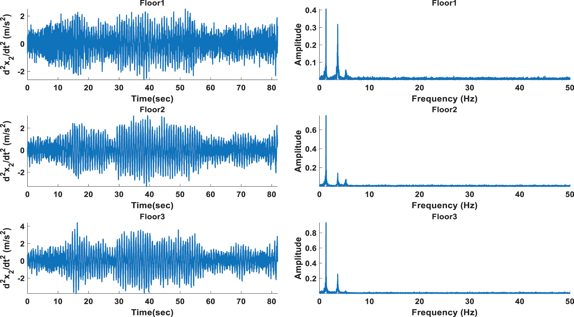
Figure 4: Acceleration from undamaged status in various stories and its corresponding spectrum

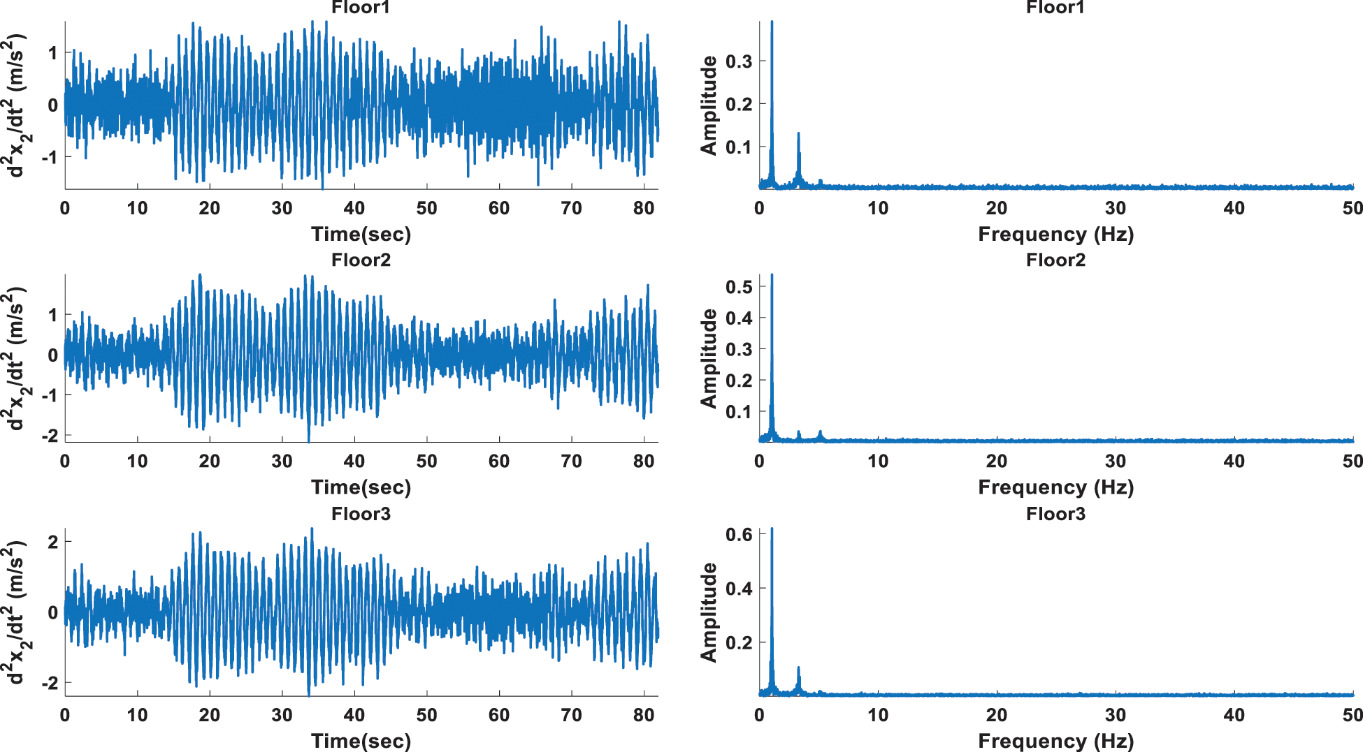
Figure 5: Acceleration from damaged status in various stories and its corresponding spectrum

Table 1: Peak values on the FFT spectrums of Floor1

5.4 Structural Modal Parameters

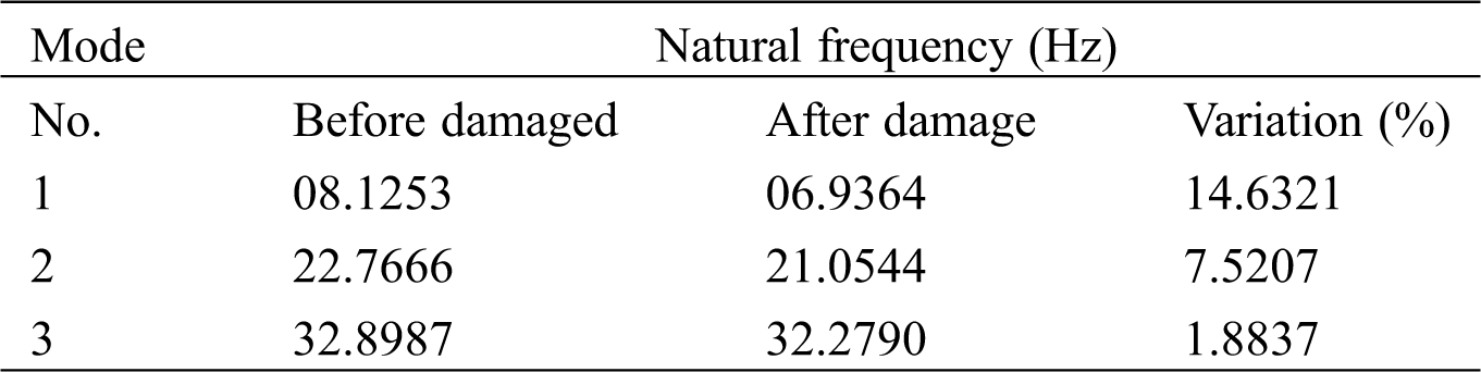
The measured acceleration responses are used to analyze and draw out the basic modal parameters (i.e., natural frequencies and mode shapes) in both damaged and undamaged scenarios. The first three modal frequencies of damaged and undamaged states are listed in Tab. 2. The comparison of natural frequencies of the un-damaged and damaged structure is carried out by calculating the relative errors, as shown in Tab. 2. It is clear that with an increase in the number of stories, the modal frequency of a frame decreases after damage. The natural frequency variation shown in Tab. 2 shows that the damaged case’s natural frequency decreased with the damage’s intensity increase.

Table 2: Natural frequency from modal analysis

6  Discussion and Results

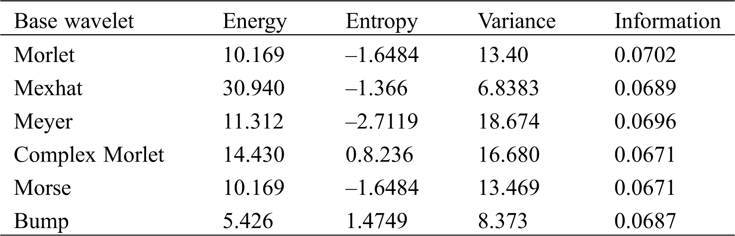
A comparative analysis among Mexican and Meyer, Morel, Morse, and Bump wavelet is conducted in this section. The signals captured from the damaged and undamaged cases on floor one have been considered. The comparative analysis is based on time-frequency representation and extracting features from wavelet coefficients based on the first scale. Tab. 3 lists the energy, entropy, and variance, sharing information values extracted from the test signal. It is seen that the Mexican wavelet shows maximum energy, and Meyer gives maximum variance, and minimum entropy, while the real Morlet wavelet provides maximum information. Also, it should be noted that real wavelet and Morse wavelet are nearly identical in their results. Also, all the functions are close in their mutual information.

Table 3: Quantitative measures

Figs. 6 and 7 show scale-time representations of floor1 for the undamaged and damaged cases, respectively, using various wavelets. These figures show whether the energy of a given frequency decreases or increases over time. Note that small scales correspond to high frequencies and large scales correspond to low frequencies in both figures. Accordingly, a small peak in the graph corresponds to the signal’s high-frequency components, and a large peak corresponds to the signal’s low-frequency components. It is noted that the analytic wavelets, Morlet, Morse, and Bump, offer the best definition in time-frequency resolution compared with non-analytic wavelets, Mexican and Meyer in both damaged and undamaged states. In Fig. 6, the analytic wavelets show the highest magnitude in scales 37 to 54 of undamaged condition, which indicates that these scales correspond to signal frequencies, which is continuous in time. There are significant changes in wavelet coefficients around these scales over time. In Fig. 7, a damaged state, it is clear that the frequency around scale 37 is shifted, which means that there is a loss of strength leading to a decrease in frequency, and most of the energy is concentrated around scale 54. The frequency shift is a typical nonlinear dynamic behavior in the signal related to energy balance in structure. It is known that the damage in the structure is a direct consequence of the energy balance within the structure [48].

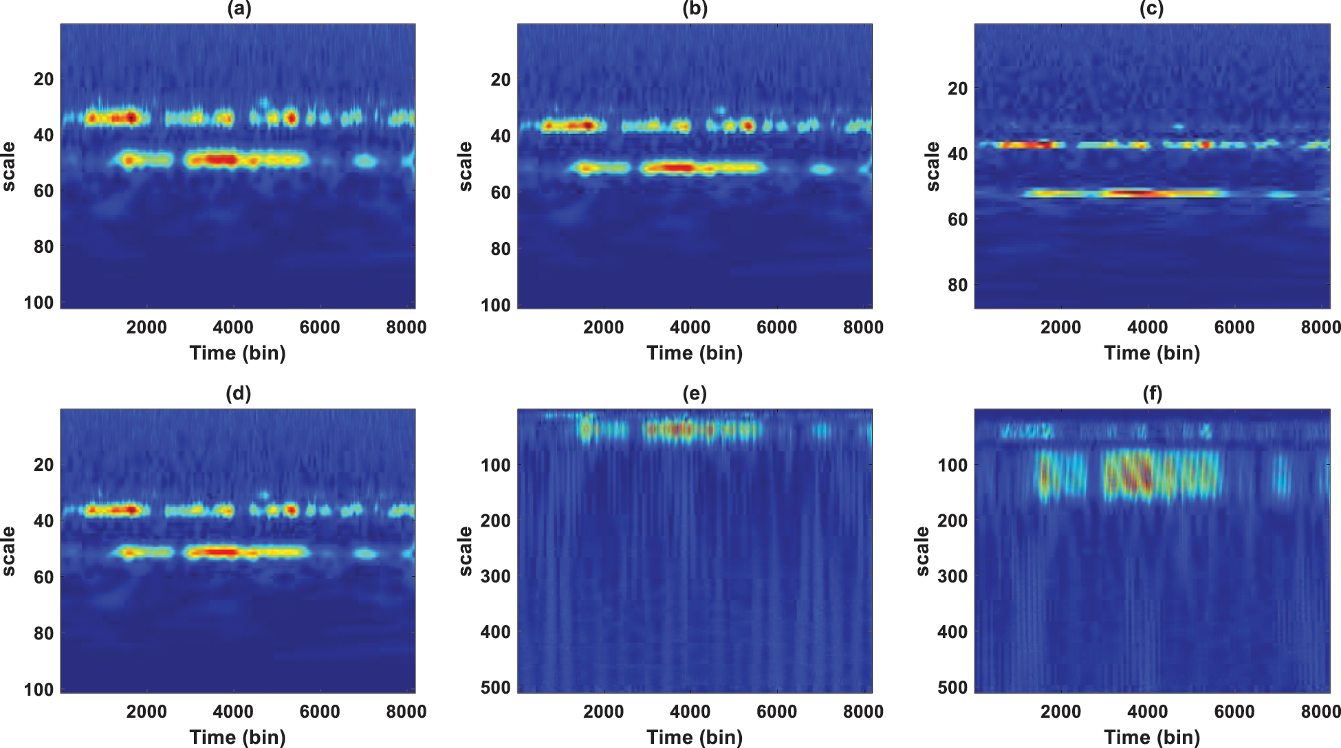
Figure 6: Time-scale representations, undamaged signal

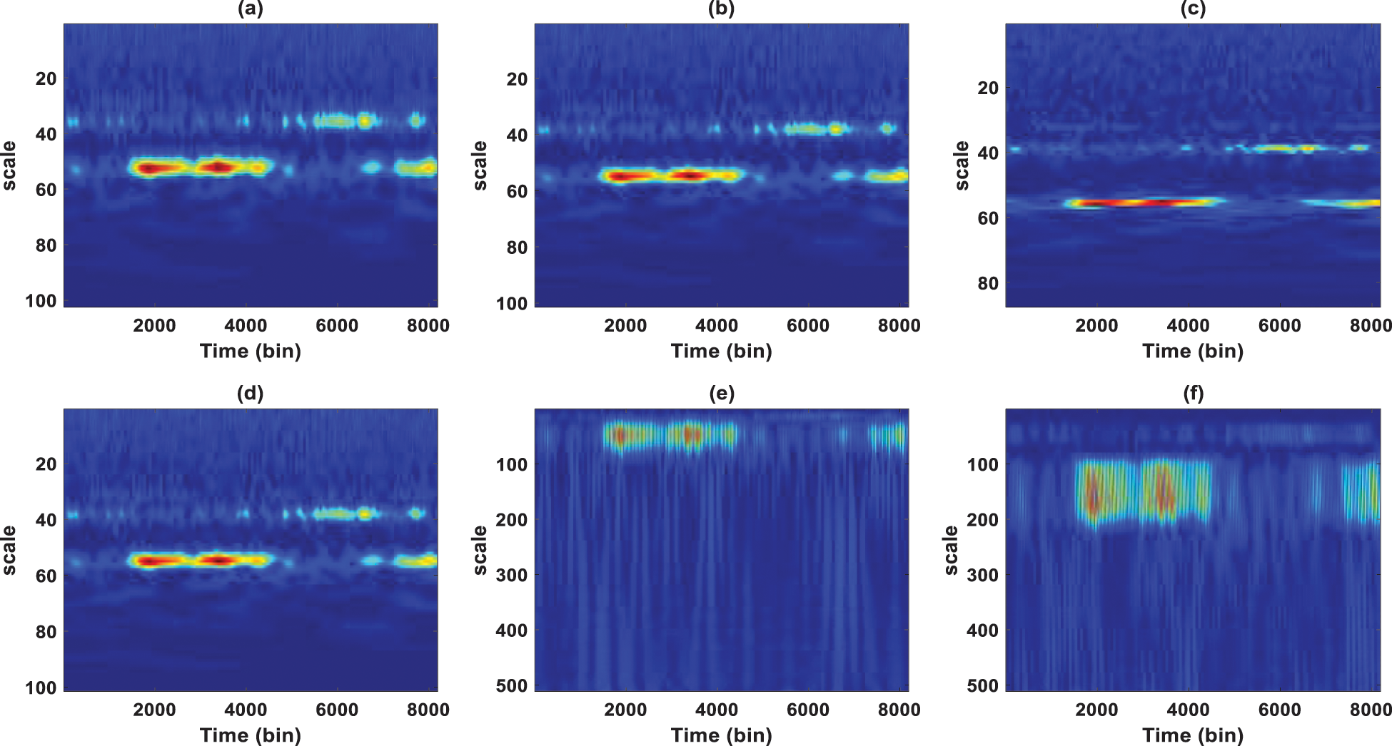
Figure 7: Time-scale representations, damaged signal

Comparing the scalograms obtained with Morlet, Morse, and Bump, it is shown that the result of Morse wavelet is nearly identical to the Morlet and all of these wavelets are nearly identical with respect to localized in time and frequency performance; however, it is shown that bump wavelet is more effective in noise separation and makes the results more amenable to interpretation. It can also be shown that the distribution of wavelet coefficient values on the time for the undamaged state is greater than the damaged state. Furthermore, it can be seen that the high value of wavelet coefficients is observed around 500 to 5000 bin for the undamaged condition and 2000 to 4000 bin for the damaged state. In general, there is a much lower level of high-frequency energy present in the signal after the damage. Finally, it can be stated that the sudden reduction of stiffness can have a significant influence on the scalogram. Based on these results, it is revealed that Morlet, Morse, and Bump functions are the best candidates for time-scale representations and more appropriate for oscillatory behavior, so these functions are used for further analysis

Figs. 8 and 9 show the 3D time-frequency representations of the signals using various analytic wavelets for damaged and undamaged states. The comparison shows that energy (bright bands) is dominated in the lower scales, i.e., there is a bright band for peaks. The blue bands result from the correlation integral to a small value due to the wavelet’s overlap with positive and negative values. It is also shown that there are some nearly steady-state fluctuations above 1 to 3 Hz and the transient events. The narrow bands represent the spikes, whereas thick bright ones represent the signal component. Besides, there are obvious changes near frequency 1 in the damaged state, which indicates how rapidly the magnitude of the wavelet coefficients changes due to damage.

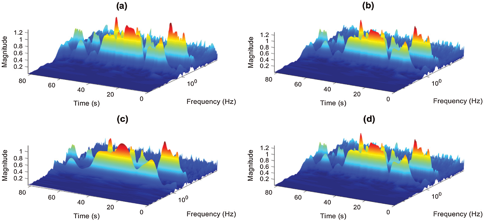
Figure 8: 3-D view of the frequency-time contour of signal, undamaged signal

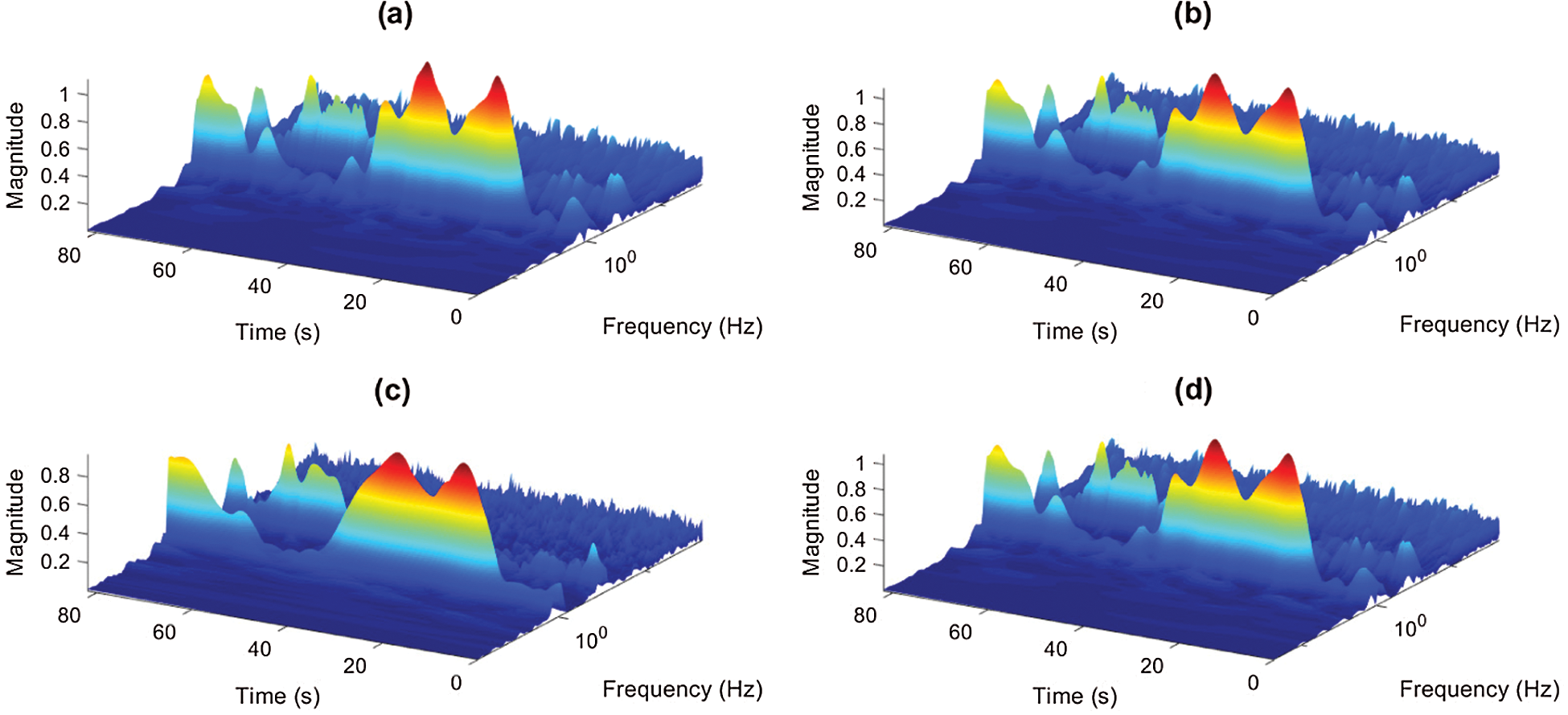
Figure 9: 3-D view of the frequency-time contour of signal, damaged signal

Fig. 10 shows the contour representations of the undamaged signal. It is evident that at scales 37, and 54 the highest magnitude can be observed. Areas with lower-density contours have weaker amplitudes, and regions with higher-density contours have higher amplitudes. The time-frequency coordinates afford a more traditional way to interpret the data. They demonstrate that most of the signal energy is focused around 37 and 54 scales. Besides, small activities at various points are observed at a contour scale of 37 and 54, which corresponds to the signal’s frequency. Fig. 11 shows the contour representations of the damaged signal. It is clear that at scales of 55 in Figs. 11a, 11b, 11d, and at scale 56 in Fig. 11c, they show the highest magnitude. Comparing Fig. 11 with Fig. 10, indicates there are switches in scales to show that some components are changed. Scale shift (or inversely frequency shift), which is a typical nonlinear behavior, was detected from the undulating contours. The frequency corresponding to scale 37 is disappeared, which is typical nonlinear behavior. In comparing damage and undamaged states, the different frequency ranges can be noticed. Most of the time, events seem to be evident, and no vertical structure is visible. It is also noted that the Bump wavelet has good frequency localization, and the deviation is higher than the others are. Thus, we can state that, Bump wavelet is the most suitable one to describe the signals’ frequency content compared to other wavelets. This proves that selecting a mother wavelet with a high correlation with the signal provides a more accurate time-frequency analysis.

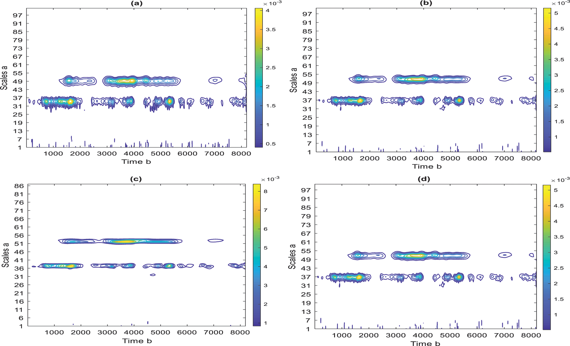
Figure 10: A contour representation of scalogram, undamaged signal

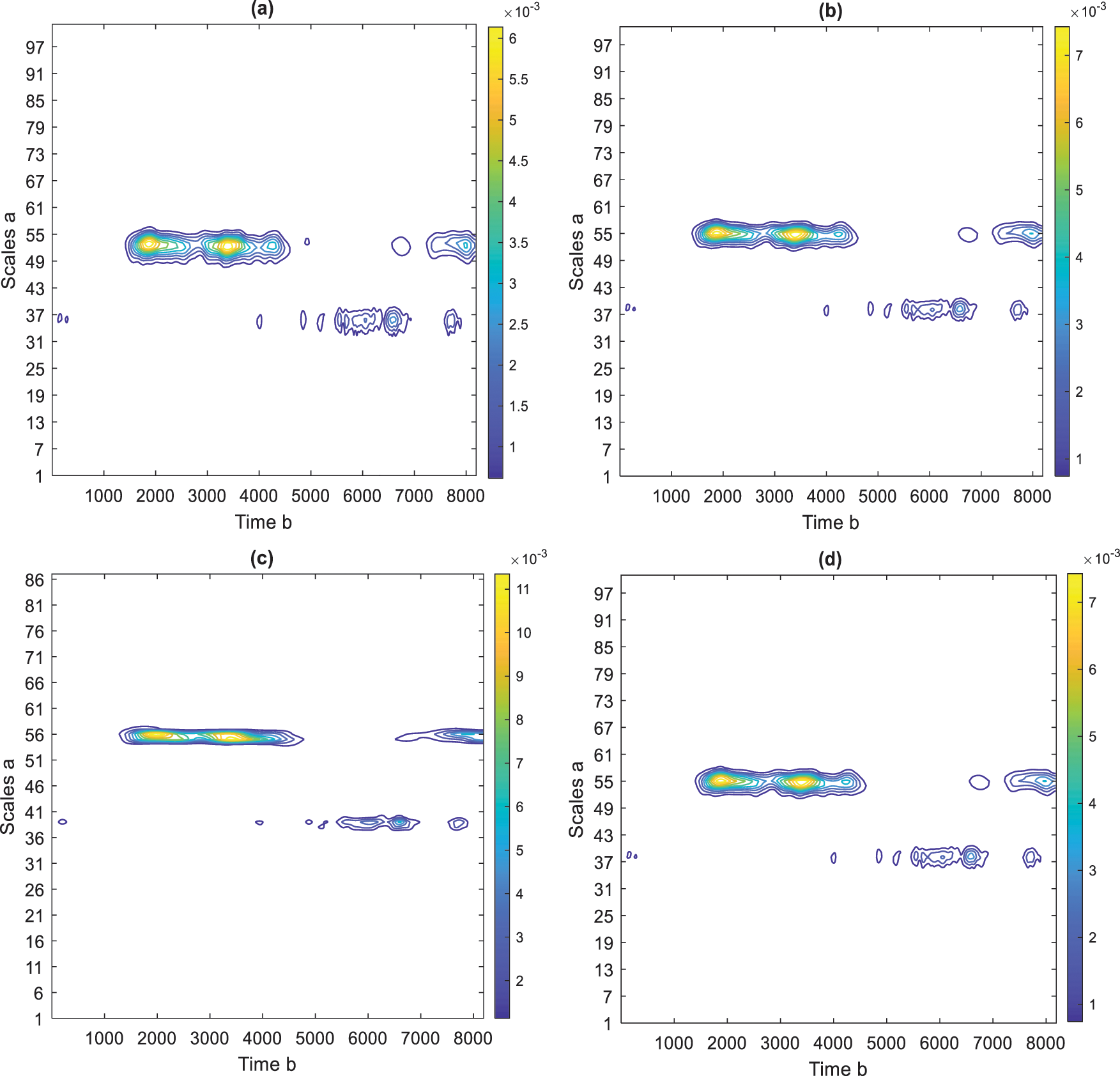
Figure 11: A contour representation of scalogram, damaged signal (a) Amor, (b) Morse, (c) Bump, (d) Morl

Fig. 12 shows finest-scale coefficients with the analyzed signal on the same plots. It is evident that the wavelet magnitudes capture the impulsive events at the exact times they occur in the signal. The Bump wavelet shows good results.

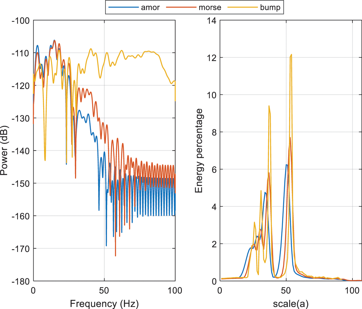
Figure 12: Finest-scale coefficients with the analyzed signal on the same plot

In order to validate the analytic wavelet function performances, power spectrum versus frequency and energy percentage versus scale are evaluated. Fig. 13 shows the power spectrum and energy percentages of Complex Morlet, Morse, and Bump. It is seen that the maximum values are given by the Bump wavelet, while the Complex Morlet wavelet shows the minimum values.

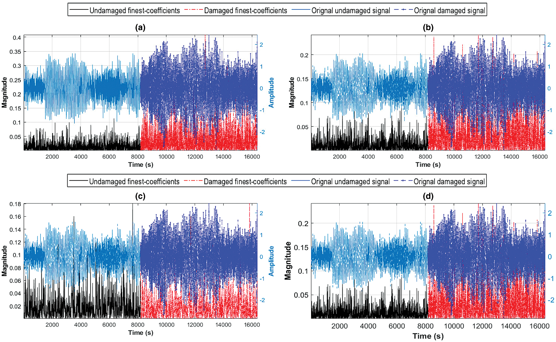
Figure 13: Power vs. Frequency (left), Energy percentage vs. scale (right)

In summary, based on the results presented herein, the analytic wavelets provide more details about time-frequency analysis. The results show that the time-frequency-based analytic wavelets are sensitive to different damage cases. They can easily extract the coefficients at a given scale that approximately correspond to the frequency of interest. This helps monitor and differentiate the transient signal frequency components that are imperative for assessing the structural status. Almost all results obtained through analyses via all analytic wavelets were close, although bump wavelets show good results. The Morse wavelet shows nearly identical to the Morlet results, and both have the advantage of allowing trade between time and frequency resolution through their parameters. In our previous studies, we found that Morse is more versatile than Morlet. The Morse wavelet can create wavelets with characteristics analogous to Morlet wavelet by adjusting Morse wavelet parameters to have a Morlet wavelet advantage and avoid its shortages. Since Morse wavelet can subsume other analytic wavelet families can create wavelets with characteristics similar to Morlet wavelet and can avoid the Morlet’s shortages, we conclude that Morse wavelet and Bump wavelet are appropriate for identifying defect induced transient components embedded within the vibration signal. They can also locate transient events or discontinuities in the data due to their time and frequency localization advantages and their ability to separate and extract quantifiable features in the time-frequency/scale domain.

7  Conclusion

In this paper, a comparative analysis for selecting the wavelet type is conducted, and subsequently, damage evaluation by wavelet scalogram is examined via numerical studies. The acceleration responses and their wavelet scalograms are utilized to evaluate the damage qualitatively. CWT has considerable potential in digital signal processing. The accelerations are obtained from the numerical models for simulated excitation under the damaged and undamaged scenario. The wavelet scalograms of these responses under external excitations are examined, and it is shown that there is a significant difference between damaged and undamaged scalograms. The process is carried out in Matlab® environment using 107 to 512 different scaled versions of the wavelet using Bump, Morse, Morlet, Mexhat and, Meyer wavelets. From scale-time representation results, it is found that the analytic wavelets show promising results compared with non-analytic wavelets. The time-frequency analysis based on complex wavelets accurately identifies the time at which various frequencies are present, it captures the instantaneous signal frequencies, and shows how the data frequency components change over time. It can be concluded that the wavelet scalogram is capable of revealing the presence of structural damage quite well, and it is recommended for time-frequency analysis for damage detection. Besides, the finest-scale components localize all the abrupt changes in the signal in time. Regarding the wavelet functions, the Bump wavelet is the most appropriate to describe the temporal organization of the signal’s frequency content compared to the other wavelets. Of course, such a conclusion cannot be generalized for all types of data processing since the type of wavelet analysis best suited for specific work depends on the data form that is used and the final objectives of the data analysis. As it is related to structural damage detection based wavelet analysis, further analytical and experimental studies on more practical cases are required for acquiring quantitative results and a more precise interpretation with results based on real field measurements.

Funding Statement: The author(s) received no specific funding for this study.

Conflicts of Interest: The authors declare that they have no conflicts of interest to report regarding the present study.

References

 1.  Sun, H., He, Z., Zi, Y., Yuan, J., Wang, X. et al. (2014). Multiwavelet transform and its applications in mechanical fault diagnosis—A review. Mechanical Systems and Signal Processing, 43(1–2), 1–24. DOI 10.1016/j.ymssp.2013.09.015. [Google Scholar] [CrossRef]

 2.  Zhao, Y., Noori, M., Altabey, W. A., Ghiasi, R., Wu, Z. (2018). Deep learning-based damage, load and support identification for a composite pipeline by extracting modal macro strains from dynamic excitations. Applied Sciences, 8(12), 2564. DOI 10.3390/app8122564. [Google Scholar] [CrossRef]

 3.  Wang, T., Altabey, W. A., Noori, M., Ghiasi, R. (2020). A deep learning based approach for response prediction of beam-like structures. Structural Durability & Health Monitoring, 14(4), 283–301. DOI 10.32604/sdhm.2020.010564. [Google Scholar] [CrossRef]

 4.  Ghiasi, R., Ghasemi, M. R., Noori, M., Altabey, W. (2019). A non-parametric approach toward structural health monitoring for processing big data collected from the sensor network. Structural health monitoring 2019: Enabling intelligent life-cycle health management for Industry Internet of Things (IIOT)—CD ROM Proceedings of the 12th International Workshop on Structural Health Monitoring, Stanford University, 2019. 10.12783/shm2019/32395. [Google Scholar] [CrossRef]

 5.  Amezquita-Sanchez, J. P., Adeli, H. (2016). Signal processing techniques for vibration-based health monitoring of smart structures. Archives of Computational Methods in Engineering, 23, 1–15. DOI 10.1007/s11831-014-9135-7. [Google Scholar] [CrossRef]

 6.  McNeill, D. K. (2009). Data management and signal processing for structural health monitoring of civil infrastructure systems. Structural health monitoring of civil infrastructure systems, pp. 283–304. Woodhead Publishing Limited. DOI 10.1533/9781845696825.1.283 [Google Scholar] [CrossRef]

 7.  Beskhyroun, S., Oshima, T., Mikami, S. (2010). Wavelet-based technique for structural damage detection. Structural Control and Health Monitoring, 17(5), 473–494. DOI 10.1002/stc.316. [Google Scholar] [CrossRef]

 8.  Hou, Z., Noori, M., Amand, R. S. (2000). Wavelet-based approach for structural damage detection. Journal of Engineering Mechanics, 126(7). DOI 10.1061/(ASCE)0733-9399(2000)126:7(677). [Google Scholar] [CrossRef]

 9.  Yan, R., Chen, X., Mukhopadhyay, S. C. (2017). Structural health monitoring: An advanced signal processing perspective. Smart sensors, measurement and instrumentation. [Google Scholar]

10. Aguirre, D. A., Gaviria, C. A., Montejo, L. A. (2013). Wavelet-based damage detection in reinforced concrete structures subjected to seismic excitations. Journal of Earthquake Engineering, 17(8), 1103–1125. DOI 10.1080/13632469.2013.804467. [Google Scholar] [CrossRef]

11. Qiao, L., Esmaeily, A., Melhem, H. G. (2009). Structural damage detection using signal pattern-recognition. Key Engineering Materials, 400–402, 465–470. DOI 10.4028/www.scientific.net/kem.400-402.465. [Google Scholar] [CrossRef]

12. Kaur, A. (2016). Commerce Mathematics comparative analysis of wavelet transform and Fourier transform, pp. 106–108. Department of Mathematics, Guru Nanak Dev University Amritsar. [Google Scholar]

13. Lei, J., Meyer, Y., Ryan, R. D. (1994). Wavelets: Algorithms & applications. Mathematics of Computation, 63, 22. DOI 10.2307/2153305. [Google Scholar] [CrossRef]

14. Rhif, M., Ben Abbes, A., Farah, I., Martínez, B., Sang, Y. (2019). Wavelet transform application for/in non-stationary time-series analysis: A review. Applied Sciences (Switzerland), 9(7), 1345. DOI 10.3390/app9071345. [Google Scholar] [CrossRef]

15. Shao, Y., Nezu, K. (2016). Extracting the symptoms of bearing faults in the wavelet domain. Proceedings of the Institution of Mechanical Engineers, Part I: Journal of Systems and Control Engineering, 218(1), 39–51. DOI 10.1177/095965180421800104. [Google Scholar] [CrossRef]

16. Kumar, H. S., Pai, S. P., Sriram, N. S., Vijay, G. S. (2014). Selection of mother wavelet for effective wavelet transform of bearing vibration signals. Advanced Materials Research, 1039(2014), 169–176. DOI 10.4028/www.scientific.net/AMR.1039.169 [Google Scholar] [CrossRef]

17. Rodrigues, A. P., Mello, G. D., Pai, P. S. (2016). Selection of mother wavelet for wavelet analysis of vibration signals in machining. Journal of Mechanical Engineering and Automation, 6(5A), 81–85. DOI 10.5923/c.jmea.201601.15. [Google Scholar] [CrossRef]

18. Fu, J., Xu, X., Chen, Y. (2017). Feature selection and optimization method based on CWT. 2017 IEEE International Conference on Signal Processing, Communications and Computing, pp. 1–4. Xiamen, China. DOI 10.1109/ICSPCC.2017.8242492. [Google Scholar] [CrossRef]

19. He, C., Xing, J. C., Yang, Q. L. (2014). Optimal wavelet basis selection for wavelet de-noising of structural vibration signal. Applied Mechanics and Materials, 578579, 1059–1063. DOI 10.4028/www.scientific.net/AMM.578-579.1059. [Google Scholar] [CrossRef]

20. Ngui, W. K., Leong, M. S., Hee, L. M., Abdelrhman, A. M. (2013). Wavelet analysis: Mother wavelet selection methods. Applied Mechanics and Materials. DOI 10.4028/www.scientific.net/AMM.393.953. [Google Scholar] [CrossRef]

21. Gaviria, C. A., Montejo, L. A. (2018). Optimal wavelet parameters for system identification of civil engineering structures. Earthquake Spectra, 34(1), 197–216. DOI 10.1193/092016EQS154M. [Google Scholar] [CrossRef]

22. Hera, A., Hou, Z. (2004). Application of wavelet approach for ASCE structural health monitoring benchmark studies. Journal of Engineering Mechanics, 130(1), 96–104. DOI 10.1061/(ASCE)0733-9399(2004)130:1(96). [Google Scholar] [CrossRef]

23. Kitada, Y. (1997). Identification of nonlinear structural dynamic systems using wavelets. Journal of Engineering Mechanics, 24, 395–410. [Google Scholar]

24. Noori, M., Wang, H., Altabey, W. A., Silik, A. I. H. (2018). A modified wavelet energy rate-based damage identification method for steel bridges. Scientia Iranica, 25(6B), 3210–3230. DOI 10.24200/sci.2018.20736. [Google Scholar] [CrossRef]

25. Zhao, Y., Noori, M., Altabey, W. A., Beheshti-Aval, S. B. (2018). Mode shape-based damage identification for a reinforced concrete beam using wavelet coefficient differences and multiresolution analysis. Structural Control and Health Monitoring, 25(1), e2041. DOI 10.1002/stc.2041. [Google Scholar] [CrossRef]

26. Fischer, W. R. (2010). Using the continuous wavelet transform to characterize differences between impact signals from non-cleated and cleated turf shoes (Ms. Thesis). Boise State University. [Google Scholar]

27. Kim, B., Jeong, H., Kim, H., Han, B. (2017). Exploring wavelet applications in civil engineering. KSCE Journal of Civil Engineering, 21(4), 1076–1086. DOI 10.1007/s12205-016-0933-3. [Google Scholar] [CrossRef]

28. Gholizad, A., Safari, H. (2017). Damage identification of structures using experimental modal analysis and continuous wavelet transform. Numerical Methods in Civil Engineering, 2(1), 61–71. DOI 10.29252/nmce.2.1.61. [Google Scholar] [CrossRef]

29. Rucka, M., Wilde, K. (2006). Application of continuous wavelet transform in vibration based damage detection method for beams and plates. Journal of Sound and Vibration, 297(3–5), 536–550. DOI 10.1016/j.jsv.2006.04.015. [Google Scholar] [CrossRef]

30. Ezra, Y. B., Lembrikov, B. I., Schwartz, M., Zarkovsky, S. (2018). Applications of wavelet transforms to the analysis of superoscillations. Wavelet Theory and Its Applications, 195. DOI 10.5772/intechopen.76333. [Google Scholar] [CrossRef]

31. Aguiar-Conraria, L., Soares, M. J. (2014). The continuous wavelet transform: Moving beyond uni- and bivariate analysis. Journal of Economic Surveys, 28(2), 344–375. DOI 10.1111/joes.12012. [Google Scholar] [CrossRef]

32. Janeliukstis, R., Rucevskis, S., Wesolowski, M., Kovalovs, A., Chate, A. (2015). Damage identification in beam structure using spatial continuous wavelet transform. IOP Conference Series: Materials Science and Engineering, 96(1), 012058. DOI 10.1088/1757-899X/96/1/012058. [Google Scholar] [CrossRef]

33. Ferrante, M., Brunone, B., Meniconi, S. (2007). Wavelets for the analysis of transient pressure signals for leak detection. Journal of Hydraulic Engineering, 133(11), 1274–1282. DOI 10.1061/(asce)0733-9429(2007)133:11(1274). [Google Scholar] [CrossRef]

34. Olhede, S. C., Walden, A. T. (2002). Generalized Morse wavelets. IEEE Transactions on Signal Processing, 50(11), 2661–2670. DOI 10.1109/TSP.2002.804066. [Google Scholar] [CrossRef]

35. Lilly, J. M., Olhede, S. C. (2012). Generalized Morse wavelets as a superfamily of analytic wavelets. IEEE Transactions on Signal Processing, 60(11), 6036–6041. DOI 10.1109/TSP.2012.2210890. [Google Scholar] [CrossRef]

36. Büssow, R. (2007). An algorithm for the continuous Morlet wavelet transform. Mechanical Systems and Signal Processing, 21(8), 2970–2979. DOI 10.1016/j.ymssp.2007.06.001. [Google Scholar] [CrossRef]

37. Cohen, M. X. (2019). A better way to define and describe Morlet wavelets for time-frequency analysis. NeuroImage, 199, 81–86. DOI 10.1016/j.neuroimage.2019.05.048. [Google Scholar] [CrossRef]

38. Torrence, C., Compo, G. P. (1998). A practical guide to wavelet analysis. Bulletin of the American Meteorological Society, 79(1), 61–78. DOI 10.1175/1520-0477(1998)079<0061:APGTWA>2.0.CO;2. [Google Scholar] [CrossRef]

39. Wachowiak, M. P., Wachowiak-Smolíková, R., Johnson, M. J., Hay, D. C., Power, K. E. et al. (2018). Quantitative feature analysis of continuous analytic wavelet transforms of electrocardiography and electromyography. Philosophical Transactions of the Royal Society A: Mathematical, Physical and Engineering Sciences, 376(2126), 20170250. DOI 10.1098/rsta.2017.0250. [Google Scholar] [CrossRef]

40. Quiñones, M. M., Montejo, L. A., Jang, S. (2015). Experimental and numerical evaluation of wavelet based damage detection methodologies. International Journal of Advanced Structural Engineering, 7(1), 69–80. DOI 10.1007/s40091-015-0084-7. [Google Scholar] [CrossRef]

41. Li, L., Cai, H., Jiang, Q. (2020). Adaptive synchrosqueezing transform with a time-varying parameter for non-stationary signal separation. Applied and Computational Harmonic Analysis, 49(3), 1075–1106. DOI 10.1016/j.acha.2019.06.002. [Google Scholar] [CrossRef]

42. Valenzuela, V., Oliveira, H. (2015). Close expressions for Meyer wavelet and scale function. Cornell University Aives. DOI 10.14209/sbrt.2015.2. [Google Scholar] [CrossRef]

43. Mi, X., Ren, H., Ouyang, Z., Wei, W., Ma, K. (2005). The use of the Mexican hat and the Morlet wavelets for detection of ecological patterns. Plant Ecology, 179(1), 1–19. DOI 10.1007/s11258-004-5089-4. [Google Scholar] [CrossRef]

44. de Oliveira, H. M., de Souza, D. F. (2006). Wavelet analysis as an information processing technique. 2006 International Telecommunications Symposium, pp. 7–12. Cornell University Aives. DOI 10.1109/ITS.2006.4433232. [Google Scholar] [CrossRef]

45. Peng, Z. K., Chu, F. L. (2004). Application of the wavelet transform in machine condition monitoring and fault diagnostics: A review with bibliography. Mechanical Systems and Signal Processing, 18(2), 199–221. DOI 10.1016/S0888-3270(03)00075-X. [Google Scholar] [CrossRef]

46. Bialasiewicz, J. T. (2015). Application of wavelet scalogram and coscalogram for analysis of biomedical signals. Proceedings of the World Congress on Electrical Engineering and Computer Systems and Science, pp. 1–8. Barcelona, Spain. [Google Scholar]

47. Gurley, K., Kareem, A. (1999). Applications of wavelet transforms in earthquake, wind and ocean engineering. Engineering Structures, 21(2), 149–167. DOI 10.1016/S0141-0296(97)00139-9. [Google Scholar] [CrossRef]

48. Cano, M. S., Sha, G. G., Gao, Y. F., Ostachowicz, W. Structural damageidentification using damping: A compendium of uses and features. Smart Materials and Sructures, 26(4), 14. DOI 10.1088/1361-665X/aa550a. [Google Scholar] [CrossRef]

This work is licensed under a Creative Commons Attribution 4.0 International License, which permits unrestricted use, distribution, and reproduction in any medium, provided the original work is properly cited.