A New Framework for Vegetation Productivity Dynamics Assessment in Patagonia: Rangeland Functional Archetypes

1  Introduction

The pastoral production systems of Argentine Patagonia are characterized by covering large areas, high heterogeneity, low animal receptivity, and high environmental variability [1], which makes their management complex. Effective assessment and grazing management decisions are essential to foster sustainability in the extensive arid rangelands of Patagonia, amid the challenges posed by climate change and desertification [2]. Additionally, land degradation assessment and monitoring tools are in high demand for intervention programs [3]. In these contexts, assessing rangelands for forage estimates is a crucial means of measuring resource conditions, allowing land managers to make informed decisions to prevent overgrazing and other processes that degrade ecosystems [4]. From an agronomy perspective, rangeland evaluations that aim to characterize the forage base—which is mostly determined by the physiognomic and floristic structure of the vegetation, primary productivity, and the annual quality of the forage—are conducted to estimate the carrying capacity of livestock [5]. The goal is to adjust the average annual animal stock load to the annual availability of forage [6].

Given the characteristics of the pastoral systems of Argentine Patagonia [7], rangeland assessments face the dilemma of prioritizing the collection of data with high spatial or temporal resolution, or generating information for large areas, making these assessments very laborious and costly in terms of time and financial resources. Rangeland assessment methods in Patagonia have primarily focused on understanding the structural elements of rangelands, considering ecological processes, grazing management, and environmental characteristics. Patch structure and floristic surveys are essential for characterizing landscapes [8–10], and rely on models supported by data obtained at plot scale or through transect measurements [11,12]. Recently, there has been an effort to extend this data collection to landscape or ecological site scales, taking spatial variation into account [13]. However, this shift requires new approaches, especially in areas with significant spatiotemporal variation [14].

Studies of the composition and biological dynamics of rangelands, with an emphasis on the processes of degradation and desertification in arid areas, served as the inspiration for another body of study [15]. According to various studies, advances in this area include landscape metric studies, analysis of vegetation and soil structure and dynamics, diversity, and patch and inter-patch types and their relationships (e.g., [16,17]). Recently, Environmental Monitoring for Arid and Semi-Arid Regions (MARAS) [18,19] has been proposed to evaluate Patagonian ecosystems both spatially and temporally. In assessing rangelands, this system looks at the floristic composition, soil cover, patch structure, inter-patch stability and function, and patch structure [2]. The process of analyzing at the regional level involves the consolidation of all sampling sites, the locations of which are determined by structural factors, primarily including geomorphology and floristic composition at the local level. This monitoring system (MARAS) is very useful for providing valuable information, but at an operational level, it is very costly both in time and economic resources.

Among the methods based on an agronomic perspective, the Net Aboveground Primary Productivity and Harvest Index Method (NAPP-HI) allows for estimating livestock carrying capacity as the ratio between forage biomass and individual animal consumption [6]. This method calculates forage availability as the product of NAPP and HI, which is the portion of NAPP that could be consumed by herbivores [20]. The most used conceptual model is that of Monteith [21], which was used in several studies of Patagonia (e.g., [22,23]). Conversely, the HI is calculated using the regional relationship between NAPP and domestic herbivore biomass, which was established by Oesterheld et al. [24]. In Patagonia, estimates of forage productivity have been tackled in a few recent studies (e.g., [25,26]). Lastly, a different approach that also uses NAPP calculated from remote sensors offers a substitute for the original method for figuring out animal carrying capacity. In this instance, coefficients are assigned to (i) the ratio of forage cover to total vegetation cover; and (ii) an animal use factor (NAPP-UF) [27], to determine the fraction of NAPP that herbivores can ingest. Notwithstanding the contribution to forage productivity, one of the main bottlenecks of these methodologies is the lack of a perspective on vegetation productivity dynamics and changes over time.

Whereas most efforts were oriented to assess vegetation structure, a profound comprehension of the temporal variation of vegetation has received less attention. The majority of traditional rangeland assessment methods focus either on data resolution (e.g., field monitoring plots or assessment plots) or area extension of information (e.g., classifications utilizing remote sensors). The limited time series of satellite data accessible until a few decades ago as well as the high expense of doing field assessments over time, are among the main restrictions for filling this gap of a functional perspective of vegetation. However, the most recent availability of satellite data series covering more than 20 years is currently advantageous as it opens up new avenues for focusing efforts on the temporal and spatial dynamics of vegetation productivity.

The functioning of vegetation refers to the dynamics of key variables such as phenology or primary productivity. This approach was proposed to discriminate biozones, using the functional characteristics of vegetation as the classification basis, mainly associated with temporal variations in net aboveground primary productivity [28,29]. Functional types serve as a precedent and characterize vegetation using the Normalized Difference Vegetation Index (NDVI) as a proxy variable for vegetation activity, through an analysis that combines statistics obtained from the annual cycle: (i) mean, (ii) range, and (iii) month with maximum value [30]. The focus was on seasonality (periodic variation throughout the year) but did not explicitly incorporate variations at other temporal scales such as intra-annual and inter-annual variations. As we mentioned above, the increase in the length of the remote sensing data series has allowed for a more comprehensive approach to studying the different time-domain frequency components that characterize the dynamics of vegetation productivity (e.g., [31]). However, this promising advance in the amount of satellite data requires new approaches to analyze and detect patterns in the dynamics that are of interest for understanding ecosystem functioning and pastoral management.

Rangeland Functional Archetypes have recently been proposed as a methodological approach to identifying temporal patterns in vegetation productivity [32]. A Rangeland Functional Archetype is an abstraction representing an ideal or typical dynamics of vegetation productivity, which is the result of a historical interaction between climate, vegetation, soil, and grazing (including pastoral management). For this work, a Rangeland Functional Archetype (RFA) is a class that represents a rangeland environment characterized by the distribution of variability in the set of frequencies that describe the dynamics of vegetation productivity, estimated from the time series of a vegetation index over a given period [33]. This study aimed to compare and evaluate the complementarity of information between two classification systems: one based on vegetation productivity dynamics, which we have termed RFA derived from remote sensing, and the other based on geomorphological features and field data at a farm level. This comparison examines the integration of remote sensing-derived archetypes with field-based classifications. We discuss the potential for RFA to enhance adaptive planning and management in Patagonian pastoral production systems in the future.

2  Materials and Methods

2.1 Study Case

The study was conducted at the INTA (National Institute of Agricultural Technology)-Pilcaniyeu Annex Field in the province of Río Negro, Argentina (Fig. 1). It is an experimental field from the institution (INTA) and, therefore, we have a wide range of information about it. There is a structural classification of landscapes from the field (see Section 2.3), widely used by the institution (INTA) in the productive farm. Situated 75 km from the city of San Carlos de Bariloche, it lies within the ecological area of Western Sierras and Plateaus, characterized by an arid and cold climate, with an average annual precipitation of 265 mm. The farm covers an area of 7345 hectares, divided into 12 main blocks (>100 hectares) and paddocks (<100 hectares).

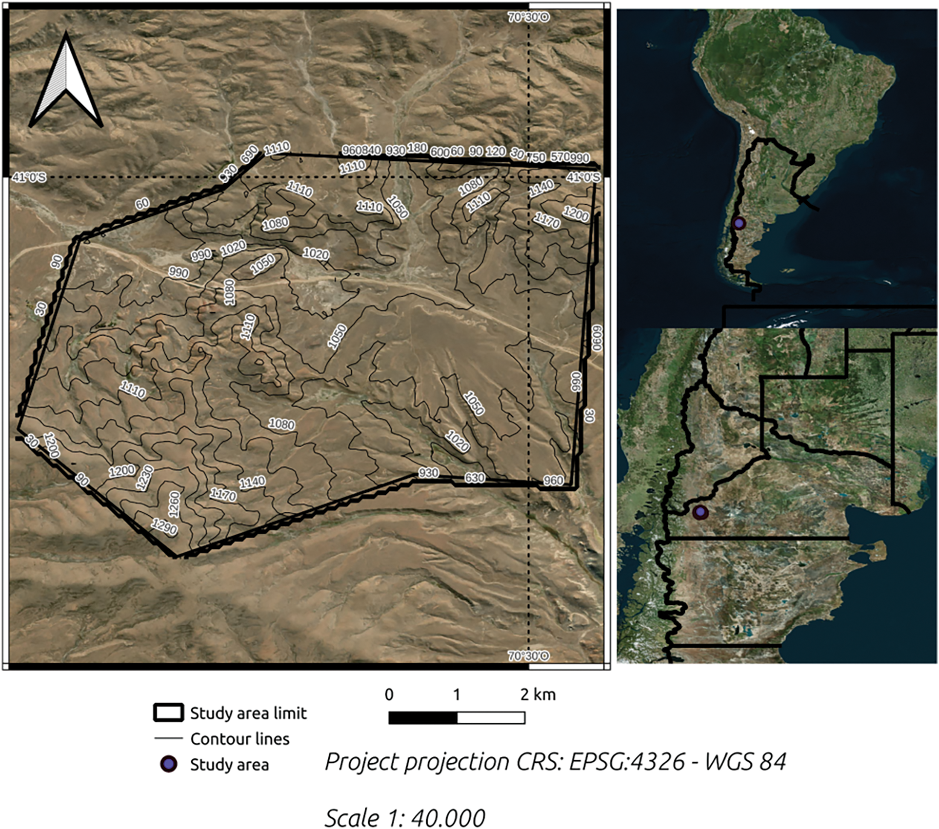
Figure 1: Location of the Pilcaniyeu annex field study area. With elevation contour lines in meters above sea level

2.2 Data

MODIS images (MODIS13Q1 product, version 6) with information on the NDVI were utilized for the period 2000–2021. The data had a frequency of every 16 days and a spatial resolution pixel of 250 m × 250 m (6.25 hectares) for the study area. These NDVI composites were downloaded from the MODIS data archive [34]. Following the methodology [32] for preprocessing the time series, we removed negative values and retained only those with a pixel reliability index of 0 or 1. Any other values were deemed invalid and excluded from the analysis. Subsequently, the NDVI data were integrated into a three-dimensional matrix (latitude, longitude, time), known as a spatiotemporal cube, which encapsulated all spatial and temporal information.

Sentinel 2 satellite images were utilized, employing bands from the visible and near-infrared spectrum with a 10-m optical resolution. Image selection prioritized quality, absence of cloud cover, and the availability of scenes corresponding to the summer season (1 January 2022), as this period observed the maximum vegetation response. The image was downloaded from the Copernicus website [35].

Details of the image used:

Product uri: S2A_msil2a_20220110t142731_n0301_r053_t19gcq_20220110t185113

Processing level: Level-2A

Product type: S2MSI2A

The digital elevation model (DEM) MDE-Ar v. 2.1 was used. This DEM has a spatial resolution of 30 m and a vertical accuracy of approximately 3 m. The model is based on quality improvement processes carried out by the National Geographic Institute using information from the ALOS Advanced Land Observing Satellite (DAICHI) project generated by the Japan Aerospace Exploration Agency (JAXA) as part of the ALOS World 3D project [36].

2.3 Classification of Landscape Units: The Traditional Methodology

For the processing of the Sentinel 2 image, it was cropped to the area of interest and subjected to unsupervised classification of 10 classes using K-MEANS. These classes were determined beforehand based on previous information from several rangeland assessments in the farm (a research station with more than 60 years of scientific studies) as well as broad information of the region. Then, based on field assessment plots the 10 original classes were corroborated and regrouped into 8 final classes [37]. The processes were mainly carried out using Quantum GIS (Open Source) software [38]. The accuracy of the cartography was confirmed by verifying classes through ground assessment plots established using biophysical scientific knowledge and previous assessments of the rangelands following this methodology [39], a total of 163 rangeland assessment plots were conducted. These evaluations involved surveying the physiognomy of the vegetation, determining the percentages of vegetation cover, and corroborating the geomorphological characteristics of the landscape units. In each rangeland assessment plot, the coverage of dominant species and total vegetation coverage were estimated, and forage productivity in kilograms of dry matter per ha year (kg*DM)/(ha*year) was determined for each landscape type. Once the landscape classes were defined and controlled, recoding was carried out to obtain a layer exclusively for wetlands. Pixels or areas not corresponding to the wetlands class were removed from this resulting layer based on field observations, and once the correction was completed, it was vectorized and overlaid with the existing landscape unit layer. Therefore, the boundaries of the wetlands unit were replaced with the newly obtained ones.

2.4 Rangeland Functional Archetypes: The New Framework

Rangeland Functional Archetypes refers to a protocol for analyzing the dynamics of vegetation productivity at the farm scale (Fig. 2). It involves using time series data of spectral indices obtained from remote sensors as a proxy variable for vegetation photosynthetic activity. We used MODIS images because their extensive time series spans over more than 20 years and is consistently measured with the same methodology. This provides an adequate spatial resolution suitable for the scale of our study. The unit of analysis is the information pixel, and the extent is the farm under study. As a first step, a cropped area of interest (i.e., space-time cube) is obtained, and then the Fast Fourier Transform [40,41] is applied to the time series of the selected vegetation index to obtain the power spectrum of each pixel within the study area. The power spectrum allows determining the distribution of signal power over a frequency range given by the length of the observation period and the temporal resolution of the data series. In the developed protocol, this range includes the frequency associated with the annual cycle, high frequencies referring to intra-annual cycles, and low frequencies linked to inter-annual cycles.

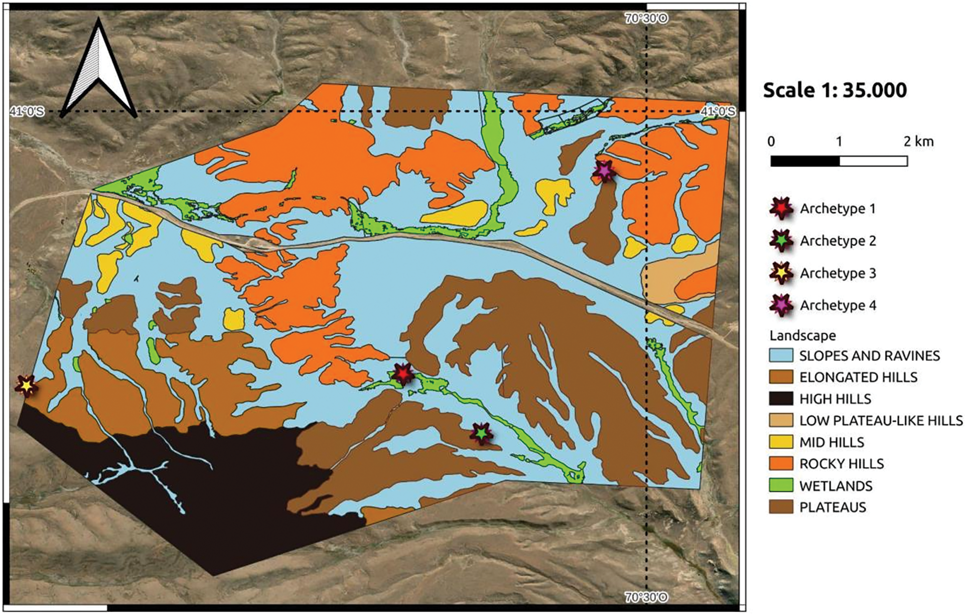
Figure 2: Map of landscape units of the study area Pilcaniyeu annex field

Subsequently, the power spectrum information is used to perform a classification through archetype analysis [42], which is a classificatory approach that identifies recurrent patterns among cases where general regularities cannot be expected, being a sensitive method to capture both extended situations and singularities [43]. To have an empirical approach to this dynamic, those cases that best represent each archetype, called archetypoids, are selected. Archetypoids are pixels with the highest individual weighting and the greatest similarity in terms of the correlation coefficient to an archetype.

Then, to understand the characteristics of vegetation dynamics in the most representative areas of a property, a Wavelet analysis is applied to the time series of these archetypoids. This characterizes the shapes of the waves contained in a series (whether regular, irregular, or asymmetrical) using different scales or time windows. Finally, the dynamics of vegetation productivity on a property are described by the relative proximity of all pixels to the most representative sites of the archetypes, defined by the archetypoids.

2.4.1 Data Preprocessing

Data preprocessing followed this procedure [44]. The images were processed by stacking the image sequence into a three-dimensional space-time matrix, hereafter referred to as the spatio-temporal cube. The NDVI is a straightforward numerical indicator utilized for remote analysis of vegetation vigor [45]. The NDVI is calculated with the following equation:

NDVI =(NIR − RedNIR) / (NIR + RedNIR) →(where 0 < NDVI > 1) (1)

where RED is visible red reflectance, and NIR is near infrared reflectance. The wavelength range of the NIR band is (750–1300 nm), and RED band is (600–700 nm). Before grouping the data, NDVI values less than 0 and measurements with a reliability index different from 0 were marked as invalid and excluded from the analysis [46].

Once the data was grouped into spatiotemporal cubes, temporal NDVI series were obtained for each pixel in the MODIS grid. Anomalies were identified in these temporal series using the find_peaks routine from the Python scientific computing library scipy [47]. Once identified, these anomalies were marked as invalid and also excluded from the rest of the analysis.

2.4.2 Power Spectra

The mean was subtracted (i.e., centered), and a linear detrending was applied to the NDVI data series for each pixel. Each individual series was transformed using the Fast Fourier Transform (FFT) [48,49]. This transformation was then converted into a power spectrum by calculating the hypotenuse between the real (cosine) and imaginary (sine) components of the transformation [50]. The spectrum was normalized by dividing it by the sum of all frequency components in the series, resulting in a normalized spectrum where the sum is one, and each individual component contains the proportion of total variability explained by each frequency. This made the variability independent of the mean and magnitude of the standard deviation of the series.

2.4.3 Archetypes Analysis

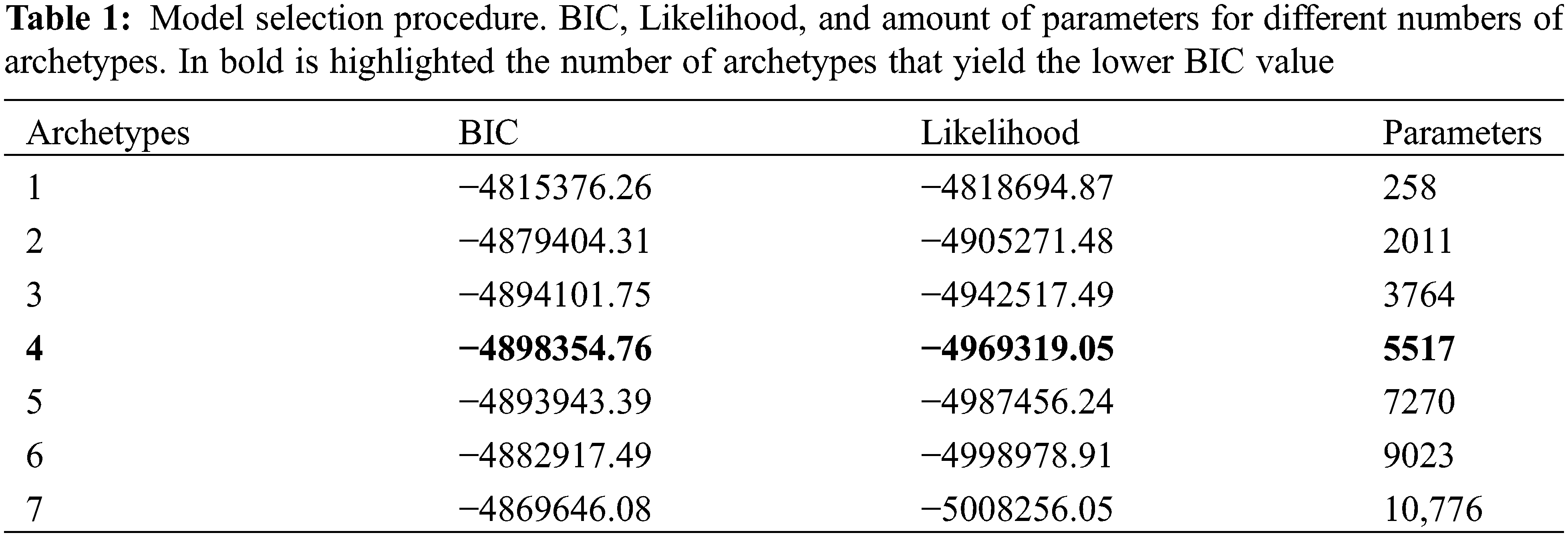
Power spectra of NDVI series for each pixel were used for an unsupervised classification through archetypes analysis [42], following this protocol [32]. Power spectra matrices were processed using the py_pcha module [51] for convex hull analysis in Python. To determine the number of archetypes, the Bayesian Information Criterion (BIC), also known as Schwarz criterion, was used [52]. The BIC value depends on the likelihood function of the model (highly related to the model’s error) and it is penalized by the number of parameters estimated. Greater number of archetypes reduce the model’s error, reducing BIC value, but increase model complexity presenting more parameters, increasing the BIC value. The analysis involved incrementing the number of archetypes until the BIC started to increase, and the resulting number of archetypes was the one with the lowest BIC [52].

As a result, two matrices were obtained: (a) one containing the archetypes themselves, meaning a matrix with theoretical power spectra corresponding to each archetypal form of the NDVI dynamics, and (b) a second one with weights, representing the coefficients by which each pixel is characterized as a linear (and convex) combination of archetypes.

Finally, archetypoids were identified, which are the most representative pixels of each archetype, defined by the highest individual weighting of a pixel with respect to an archetype and the greatest linear correlation between the archetype and the power spectrum of the temporal series of that pixel. These archetypoids contain the most similar power spectra between the observed series and the theoretical archetypes and were used for the next stage.

2.4.4 The Time-Frequency Analysis of the NDVI Series

The original NDVI series for each archetypoid were selected. For each case, the data series were re-centered without removing the trend. Subsequently, noise was eliminated, and filtering was performed using the wavelet technique. The pixel value series were decomposed into a series of Gabor atoms (i.e., sinusoidal functions localized in time through a Gaussian window) using the Basis Pursuit Denoising procedure [53]. This resulted in an optimal decomposition of the time series in terms of the number of parameters and information content of the original series. This procedure generated a time-frequency version of the Lomb-Scargle periodogram.

Once the wavelet transform was calculated, residuals were obtained by subtracting the reconstructed series from the original series. An Auto-Regressive Moving Average (ARMA) [54], model was then applied to these residuals to separate correlated noise (or colored noise) (RC) from white noise (i.e., without serial correlation) (RB) in the residual series. Thus, the stochastic component of the series was characterized, consisting of correlated (or colored) noise (RC), and uncorrelated (or white) noise (RB), corresponding to the remaining stochasticity and measurement errors. The procedure was performed in two steps. Firstly, the order of the two components of the ARMA model was calculated: the order of the autoregressive process (denoted as p) and the order of the moving average process (denoted as q). This was done by fitting increasingly complex models until the Akaike Information Criterion (AIC) started to increase [55]. The procedure began with the white noise model (ARMA (0,0)), and each step increased one order, testing all combinations of p and q and calculating the corresponding AIC. Once the best ARMA (p, q) model was selected, the RC time series was calculated using the predicted values of the ARMA fit, and the RB time series was obtained from the residuals of the procedure.

Once the decomposition (wavelets + ARMA) was obtained, the series was reconstructed according to the following criteria proposed [32]: (1) Trend, the series was reconstructed using Gabor atoms whose characteristic wavelength is greater than or equal to the length of the time series; (2) Low Frequencies, the series was reconstructed using only atoms with a wavelength shorter than the length of the series but greater than 4 years; (3) Medium Frequencies, the series was reconstructed using atoms with a wavelength between 1 and 4 years; (4) Annual Cycle, the series was reconstructed with atoms whose wavelength was one year or its harmonic series (i.e., integer multiples of 1/year); (5) High Frequencies, the series was reconstructed with atoms with wavelengths less than one year but not part of the harmonic series of the year; (6) White Noise, the series was reconstructed using the residuals from the ARMA analysis, obtaining only white or uncorrelated noise, a remnant from the analysis; (7) Colored Noise, the series was reconstructed using the coefficients of the ARMA model, containing only autocorrelated noise.

2.5 Comparison between the Structural and Functioning of Rangelands

Boxplots of the Rangeland Functional Archetypes weights were used to evaluate the relationship between the archetypes and the structural landscape units classification. If a structural landscape class exhibits high weight values of a specific archetype, then this archetype is capturing the dynamics of that class. Moreover, since there is a relationship between elevation and structural and functional aspects of rangeland ecosystems [56], a visual analysis was done comparing the high archetypes weights (over 0.5) and the pixel elevation (meters above sea level).

3  Results

3.1 Landscape Units and Vegetation Physiognomy Types

The study area was classified into eight (8) classes of landscape units defined by the geomorphology. The physiognomic composition found in each landscape unit is described as follows: (1) Wetlands: prairies with 80% to 100% of vegetation cover, (2) Low Plateau-like Hills: comprising a medium rangeland shrub steppe with 40%–50% of vegetation cover, (3) Slopes and Ravines: comprised of a medium rangeland shrub steppe with 40% of vegetation cover, a low rangeland shrub steppe with 45% of vegetation cover, a rangeland shrub steppe with 30% of vegetation cover, and a medium rangeland steppe with 25% of vegetation cover, (4) Elongated Hills: comprising a sub-shrub rangeland steppe with 30% of vegetation cover and a low rangeland shrub steppe with 45% of vegetation cover, (5) High Hills: comprising a low rangeland shrub steppe with 30% of vegetation cover and a low rangeland shrub steppe with 25% of vegetation cover, (6) Mid Hills: comprising a low rangeland shrub steppe with 40% of vegetation cover, (7) Rocky Hills: comprising a low rangeland shrub steppe with 40% of vegetation cover, a low rangeland shrub steppe with 35% of vegetation cover, and a medium rangeland shrub steppe with 35% of vegetation cover, (8) Plateaus: comprised of a low rangeland shrub steppe with 35% of vegetation cover, a medium rangeland shrub steppe with 35% of vegetation cover, a low rangeland shrub steppe with 35% of vegetation cover, and a medium rangeland shrub steppe with 40% of vegetation cover.

The wetlands in the Patagonia region are located along drainage lines, which, due to their relatively low position, receive contributions of surface or subsurface water. This increased availability of water leads to the development of azonal soils and vegetation types. They are the environments with the highest forage production per area.

3.2 Rangeland Functional Archetypes

Four Rangeland Functional Archetypes were identified in the study site (Table 1), using the lower BIC value as the selection criterion.

The four archetypes differed in terms of their power spectrum, although all exhibited peaks associated with the annual cycle and biennial periodicities (Fig. 3). Archetype 1 showed a predominance of the annual cycle, with lesser variability in higher frequencies (Fig. 3A). Archetype 2 was characterized mainly by high frequencies, above the magnitude of the annual cycle, indicating a complex annual cycle (Fig. 3B). Archetype 3 also featured a predominance of high frequencies, similar to Archetype 2, but with greater amplitudes and a stronger presence of frequencies around 1–2 months (Fig. 3C). Lastly, Archetype 4 was characterized by high frequencies and a peak around 2 years, predominating in magnitude above the annual cycle (Fig. 3D).

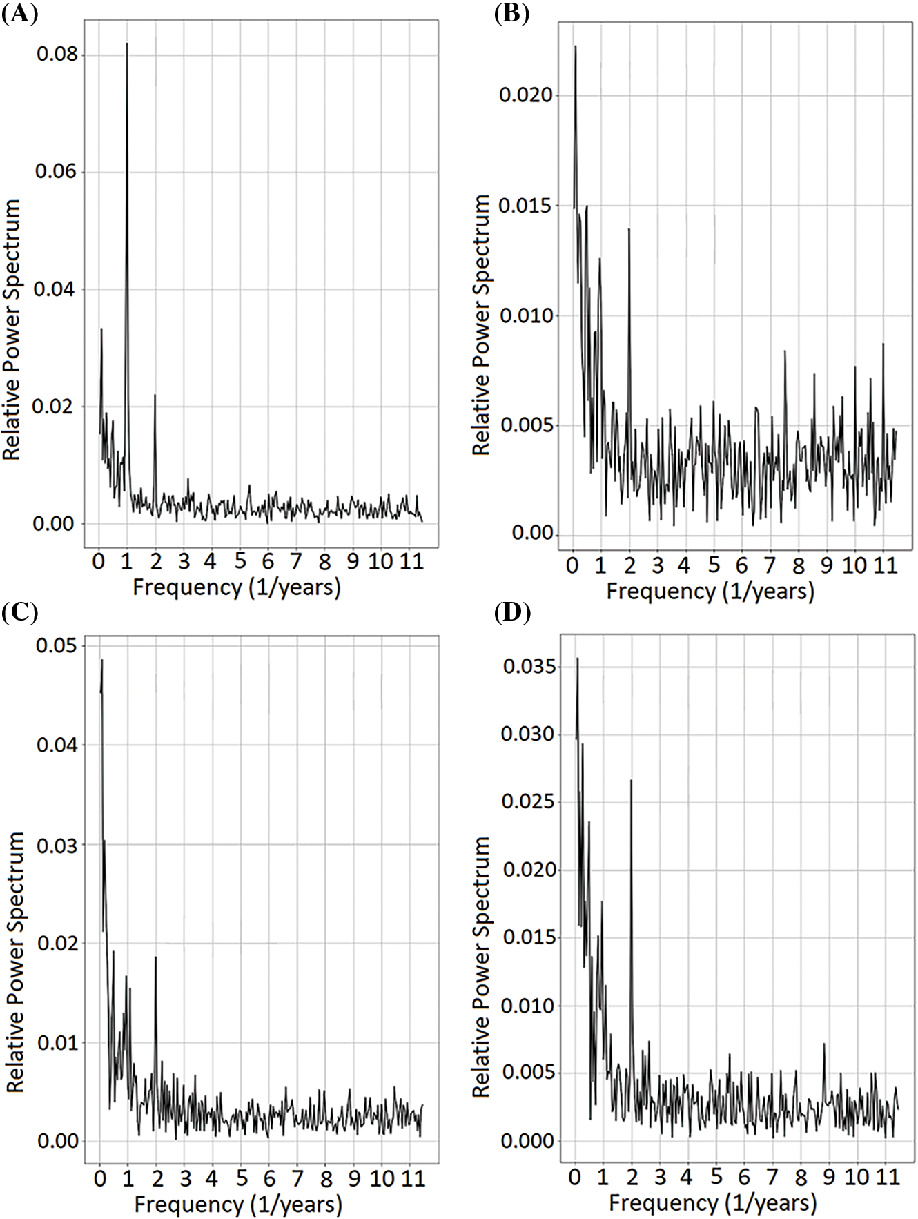
Figure 3: Power spectra for different frequencies of NDVI series of the selected arquetypoids. Panel (A) Archetype 1, (B) Archetype 2, (C) Archetype 3 and (D) Archetype 4

Geographically, archetype 1 was located in the center of the farm with a longitudinal distribution and partly in the western area (Fig. 4A). Archetype 2 does not exhibit a clearly defined distribution pattern within the farm (Fig. 4B). However, its peak values are concentrated around areas of significant human disturbance, such as the ranch area, roads, and forest plantations. Archetypes 3 and 4 will be located in the southwest and northeast part of the farm, respectively (Fig. 4C,D).

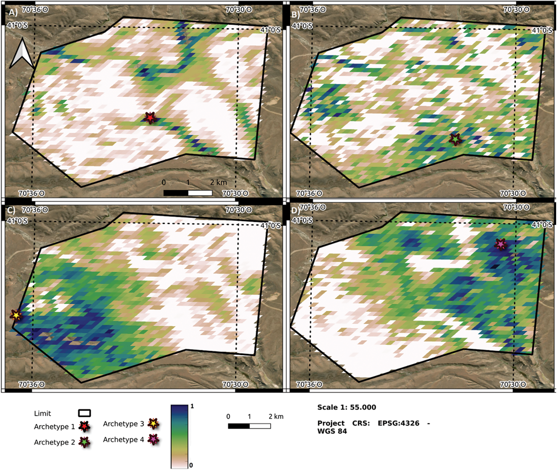
Figure 4: Classification of pixels in the study area according to the weight of each one with respect to Archetype 1 (A), Archetype 2 (B), Archetype 3 (C), Archetype 4 (D). The lighter colors correspond to lower pixel weights with respect to the archetype (White = 0), and the darker ones to higher weights (Blue dark = 1). The star identifies the location of the most representative pixel of archetype or archetypoids

3.3 Time-Frequency Analysis of Archetypes

Archetype 1. The trend peaked around the years 2002–2004 and then declined slowly to a minimum in 2012, stabilizing thereafter (Fig. 5A). Variability explained by medium and low frequencies was higher than the trend, and was significantly impacted by a disturbance in 2011 related to the ashfall from the Caulle-Puyehue Volcanic Complex eruption [57], with effects extending until 2013 (Fig. 5B,C). The annual cycle exhibited changes between a distinctly seasonal pattern and a bimodal cycle, with its amplitude increasing until 2010–2012 and then beginning to decrease (Fig. 5D). High frequencies recorded the disturbance occurring mid-study period, affecting their subsequent behavior (Fig. 5E). Noise remained constant throughout the period, with uncorrelated noise being more prominent (Fig. 5F,G).

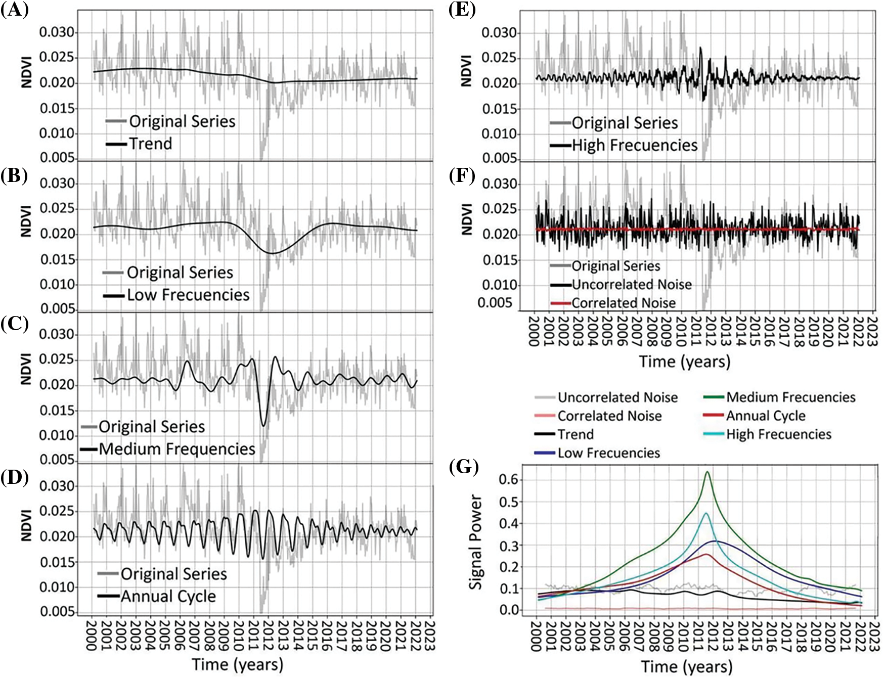
Figure 5: NDVI time-series decomposition for Archetypoid 1. Original time-series is shown in light-gray. In black line shows the decomposition of: trend (panel A), low frequencies (panel B), medium frequencies (panel C), annual cycle (panel D), high frequencies (panel E), and uncorrelated noise (panel F). Red line in panel F shows the correlated noise. Panel (G) shows the power signal over time of the different frequencies

Archetype 2. The trend explained a very small portion of the variance, with minimum values in its amplitude around the dates of the disturbance in 2011 (Fig. 6A). Low and medium frequencies followed a similar pattern as described for Archetype 1, explaining the most variance (Fig. 6B,C). The annual cycle changed over the study period, transitioning gradually from a bimodal cycle with differences between its peaks to an approximately sinusoidal bimodal cycle around 2014 (Fig. 6D). High frequencies exhibited an increase in amplitude following the 2011 disturbance and a peak in amplitude between 2020 and 2021 (Fig. 6E). Noise remained constant throughout the period, with uncorrelated noise being more prominent (Fig. 6F,G).

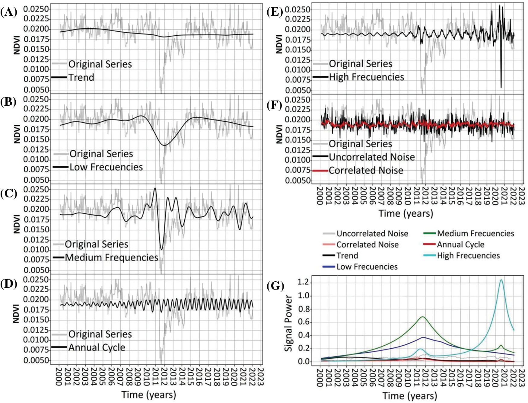
Figure 6: NDVI time-series decomposition for Archetypoid 2. Original time-series is shown in light-gray. In black line shows the decomposition of: trend (panel A), low frequencies (panel B), medium frequencies (panel C), annual cycle (panel D), high frequencies (panel E), and uncorrelated noise (panel F). Red line in panel F shows the correlated noise. Panel (G) shows the power signal over time of the different frequencies

Archetype 3. The dynamics exhibited a trend and low to medium frequencies similar to Archetype 1, but with greater amplitudes (Fig. 7A–C). The annual cycle displayed a bimodal behavior that increased in amplitude until around 2010 and then remained constant (Fig. 7D). High frequencies saw an increase in amplitude around the disturbance in 2011 (Fig. 7E). The noise remained constant in both magnitude and structure throughout the period, with uncorrelated noise also being more prominent (Fig. 7F,G).

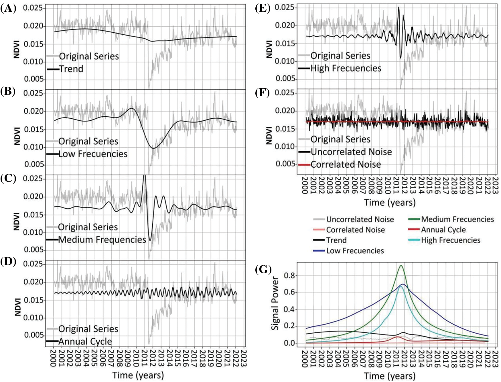
Figure 7: NDVI time-series decomposition for Archetypoid 3. Original time-series is shown in light-gray. In black line shows the decomposition of: trend (panel A), low frequencies (panel B), medium frequencies (panel C), annual cycle (panel D), high frequencies (panel E), and uncorrelated noise (panel F). Red line in panel F shows the correlated noise. Panel (G) shows the power signal over time of the different frequencies

Archetype 4. The dynamics showed a trend and low to medium frequencies similar to Archetype 1, although the medium frequencies maintained higher amplitudes after the disturbance in 2011 compared to before (Fig. 8A–C). The annual cycle exhibited a bimodal behavior that slightly increased in amplitude and tended towards a sinusoidal pattern, which persisted roughly between 2011 and 2019 (Fig. 8D). High frequencies maintained almost negligible amplitudes until the disturbance in 2011, after which they peaked and then stabilized at a higher value (Fig. 8E). As in the previous cases, noise remained constant throughout the period, with uncorrelated noise being more prominent (Fig. 8F,G).

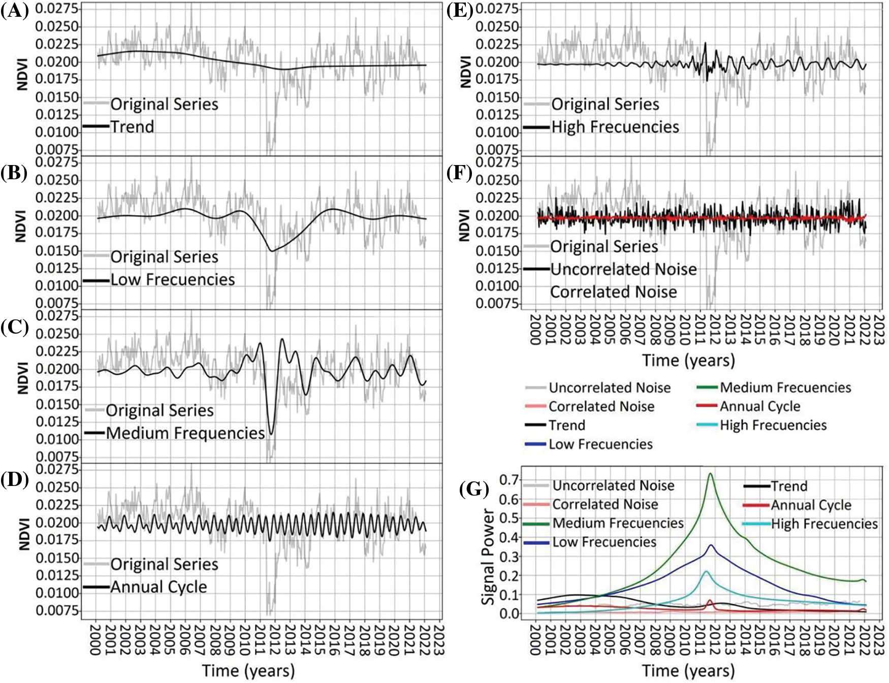
Figure 8: NDVI time-series decomposition for Archetypoid 4. Original time-series is shown in light-gray. In black line shows the decomposition of: trend (panel A), low frequencies (panel B), medium frequencies (panel C), annual cycle (panel D), high frequencies (panel E), and uncorrelated noise (panel F). Red line in panel F shows the correlated noise. Panel (G) shows the power signal over time of the different frequencies

3.4 Relationship between Landscape Classification and Productivity Dynamics

In order to further study the RFA relationships, they were compared with the landscape units (Fig. 9) and with the terrain altitude (Fig. 10) of the representative pixels. Functional Archetype 1 had a greater relative weight associated with the wetland landscape unit and, also, with lower elevation areas. This association was expected since wetlands are generally located above drainage lines in relatively low positions, thus receiving surface or underground water contributions. Regarding Archetype 2, no relationship or association with the landscape units were found, which might reflect a combination or mixture of the other three archetypes. Archetype 3 had a greater relative weight in areas associated with the landscape unit of high hills and elongated hills. In turn, it recorded the greatest representation in areas of high elevation. Finally, Archetype 4 had a greater relative weight in areas associated with the landscape unit of low plateau-like hill, plateaus, rocky hills, and slopes and ravines. This archetype was located in high areas but at a lower elevation than Archetype 3.

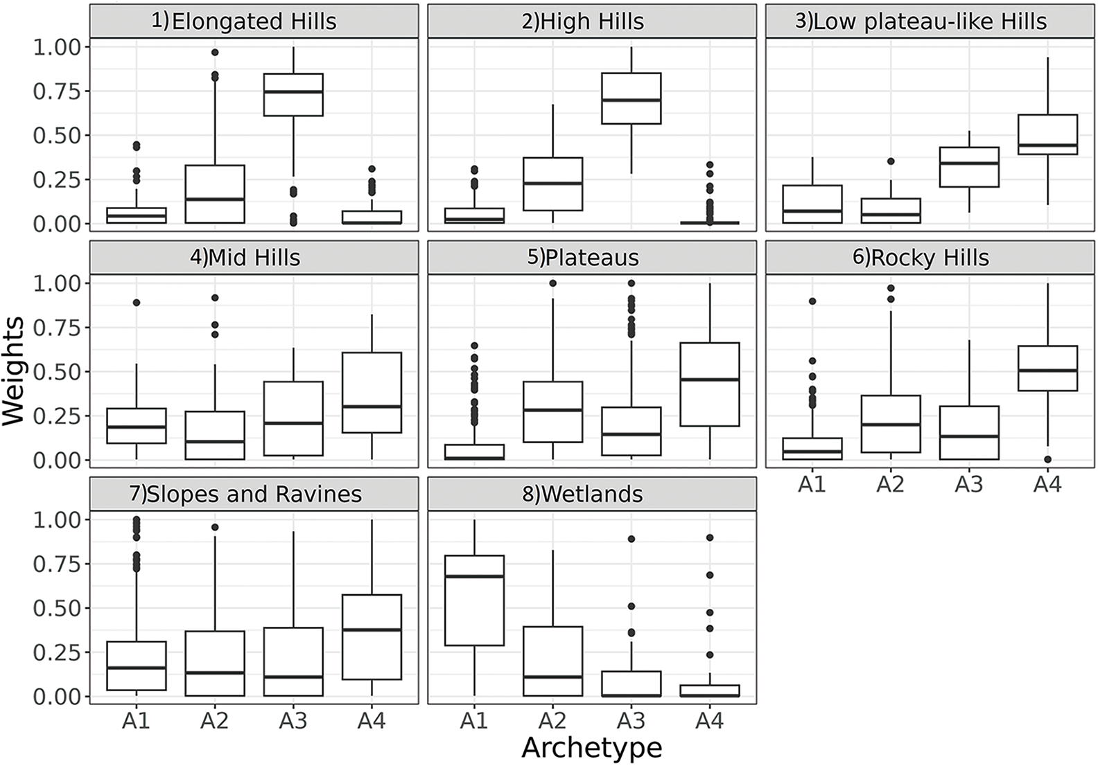
Figure 9: Boxplot of pixel’s weights of each Rangeland Functional Archetype for each structural landscape unit: (1) Elongated Hills, (2) High Hills, (3) Low plateau-like Hills, (4) Mid Hills, (5) Plateaus, (6) Rocky Hills, (7) Slopes and Ravines, (8) Wetlands

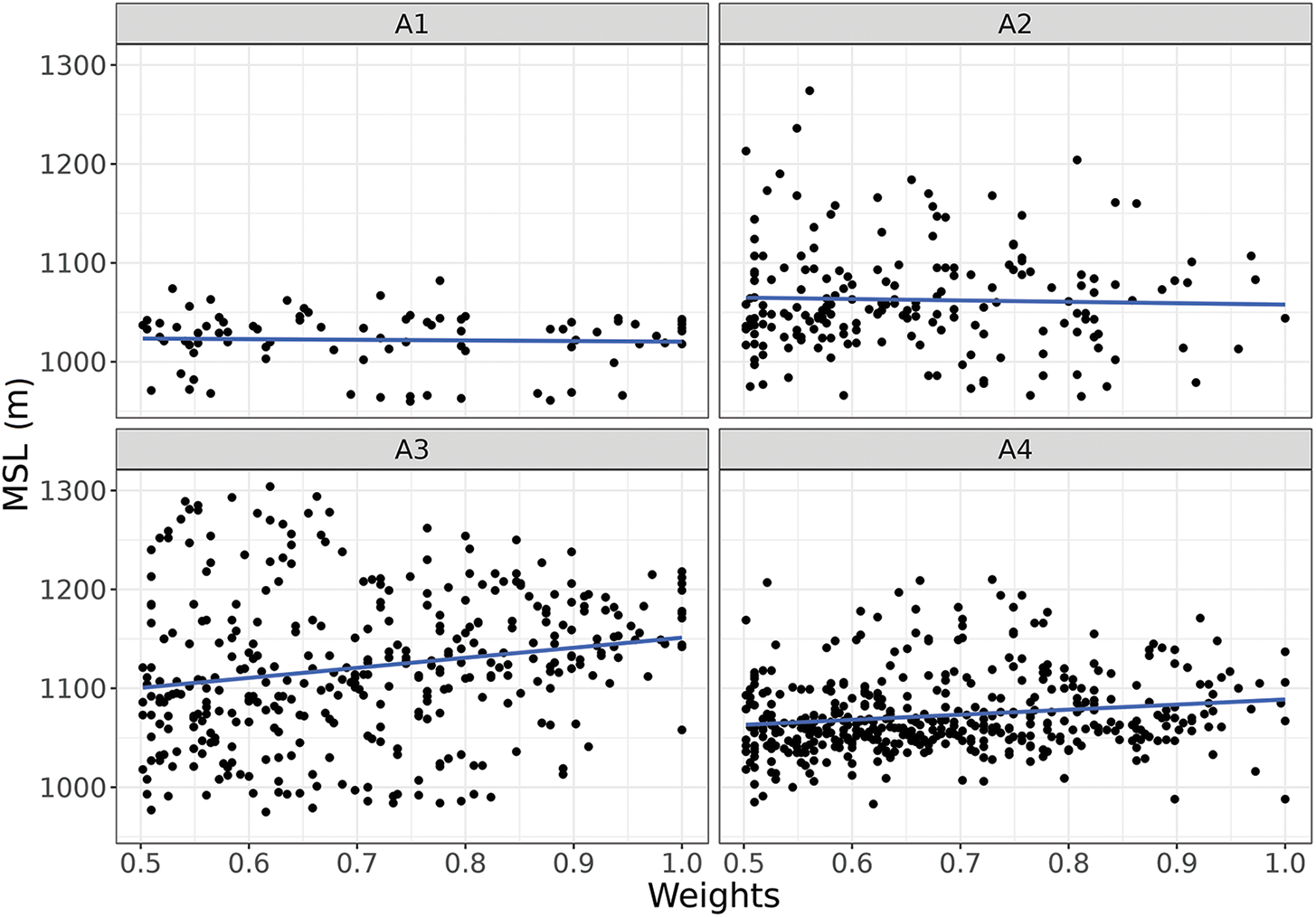
Figure 10: Scatter-plot of high archetypes weights (over 0.5; X-axis) and the pixel elevation (Y-axis) in meters above sea level (MSL). Each panel corresponds to the weight of a different archetype. The blue line shows the mean height for each archetype: 1022 m for Archetype 1, 1063 m for Archetype 2, 1122 m for Archetype 3, and 1073 m for Archetype 4. Panel references: (A1) Archetypoid 1, (A2) Archetypoid 2, (A3) Archetypoid 3 and (A4) Archetypoid 4

4  Discussion

The dynamics of vegetation productivity, discriminated using the Rangeland Functional Archetypes, was analyzed in a pastoral farm in Patagonia to compare and evaluate its complementarity with structural studies such as the differentiation of landscape units, classified according to their geomorphology. In general terms, the functioning of the vegetation was correlated with the landscape units at a regional scale. The Rangeland Functional Archetypes protocol proved to be sensitive enough to identify and characterize differences in some frequencies of the NDVI series associated with certain landscape units. For example, archetype 1 was strongly associated with wetlands, while Archetype 3 was associated with hills and higher elevation areas (Fig. 9). Archetype 4 also showed similarity with various landscape units such as plateaus, associated with high elevations, although lower than those of Archetype 3 (Fig. 9). Hence, these results emphasize that changes in time of vegetation productivity should be used as a classificatory factor and not solely as a descriptive variable. The ecosystems of the study area had undergone significant changes influenced by external environmental factors, such as the climatic regime change in Northern Patagonia around 2006–2008 towards conditions of higher temperature and reduced precipitation [58]. Furthermore, in 2011, the ecosystem experienced an abrupt disturbance caused by a volcanic ashfall [57], which also negatively affected pastoral production [59]. This event accentuated the challenges posed by the current climate transition, further impacting the ecological dynamics of the area. These environmental processes and events have acted as drivers at a regional scale, hierarchically modulating the dynamics of vegetation productivity (mainly in the trend and low frequencies) for the last 20 years. Added to the environmental processes and events, the ecological conditions of the site, the historical management practices, and degradation processes would influence the response in the vegetation dynamics [60,61], which could be reflected in frequencies other than the annual cycle, such as either high or medium frequencies or even in the noise component. These results suggest that more research is needed in the study of vegetation dynamics from a more integrative perspective.

More than 30 years ago, the classification of vegetation functioning was proposed with the idea of discriminating biozones of interest through observations of temporal variations in the aboveground net primary productivity [27]. NDVI was frequently used as a proxy variable [31] but with a main focus on annual seasonality, which was based on a stationary approach. With broad temporal analyses, we can address either multi-annual (inter-annual) periods or smaller periods that allow incorporating non-seasonal intra-annual variation and noise components [32,62]. This more detailed description of differences in rangeland productivity dynamics is a powerful tool, especially when it comes to studying non-stationary changes in vegetation [35] and spatiotemporal transitions [63]. In turn, the most representative sites of vegetation dynamics (i.e., archetypes, Fig. 4) can be used to orient field monitoring plots for rangeland assessments as well as for testing the implementation of management decisions and adapting proposals to changes in climatic variables [63,64]. These key sites could also be prioritized for the installation of new monitoring plots for the long-term study of vegetation, such as those proposed by the MARAS [18,19], as well as for studies of vegetation patches and interpatches monitored by sensors mounted on Unmanned Aerial Vehicles (UAVs) [65].

Incorporating information about these changes would be beneficial for decision-making in farms, enabling the implementation of adaptive pastoral management and helping to identify areas that could have different grazing schemes. The combination of a structural classification (based on landscape units) and a functional classification (based on RFAs) offers an innovative perspective for its application in the pastoral systems of Patagonia. In the studied farm, the productivity dynamics were mainly explained by biennial and intra-annual cycles in the steppes, whereas the annual cycle prevailed in the wetlands. Pastoral management decisions could consider these medium-term oscillations, characterized by two-year phases (more relevant in steppes located in lower altitude areas), to anticipate changes in the stocking rates or grazing requirements that may fluctuate according to this pattern. Additionally, the biennial dynamics could be included in the assignment of resting periods for different rangelands. Finally, the intra-annual behavior (cycles of less than six months) reflects an opportunistic dynamic of productivity (especially in steppes) that could be considered in pastoral planning to promote flexibility in management, aiming to take advantage of these pulses.

The Rangeland Functional Archetypes framework can help to address the necessary balance between the effort to obtain quality information on the coverage of the studied area and increasing the breadth of the period considered [3]. Given that pastoralism in Patagonia is based on the usage of wide extensions and great heterogeneity [1], it is necessary to search for new tools that help reduce operating costs and provide novel solutions for future rangeland evaluations. As a new procedure, certain issues need more research, and other factors could be further incorporated such as slope orientations, slope degrees, and soil types. Therefore, we consider it necessary to delve deeper into future research to expand knowledge and help shed light on the vegetation response to environmental changes as well as rangeland management decisions. We emphasize that the combination of structural classifications [66] and a functional classification [32,33] could offer a starting point for future integrative solutions and research associated with the more efficient management and monitoring of Patagonia’s rangelands.

Acknowledgement: None.

Funding Statement: This study was carried out with funding from the National Institute of Agricultural Technology (INTA-I099) and BIRF-8867 (GIRSAR 2.3.3, Project 12, 2022).

Author Contributions: The authors confirm contribution to the paper as follows: study conception and design: Mario Eugenio Sello, Rafael Adrian Maddio, Octavio Agusto Bruzzone, Marcos Horacio Easdale; data collection: Daniel Alejandro Castillo, Mario Eugenio Sello, Rafael Adrian Maddio; analysis and interpretation of results: Mario Eugenio Sello, Rafael Adrian Maddio, Santiago Ignacio Hurtado, Daniel Alejandro Castillo, Daiana Vanesa Perri, Octavio Agusto Bruzzone, Marcos Horacio Easdale; draft manuscript preparation: Mario Eugenio Sello, Rafael Adrian Maddio, Santiago Ignacio Hurtado, Daniel Alejandro Castillo, Daiana Vanesa Perri, Octavio Agusto Bruzzone, Marcos Horacio Easdale. All authors reviewed the results and approved the final version of the manuscript.

Availability of Data and Materials: MODIS images are open and found on the US Geological Survey (USGS) website [38]. The digital elevation model is available on the IGN website [40]. Sentinel-2 satellite images are open access and available on the web through the Copernicus Data Space Browser [39]. The layers of landscape units are not available because it is for private use of the institution (INTA).

Ethics Approval: Not applicable.

Conflicts of Interest: The authors declare that they have no conflicts of interest to report regarding the present study.

References

1. Ormaechea SG, Peri P, Cipriotti P, Distel R. El cuadro de pastoreo en los sistemas extensivos de Patagonia Sur. Percepción y manejo de la heterogeneidad. Ecol Austral. 2019;29(2):174–84 (In Spanish). doi:10.25260/ea.19.29.2.0.829. [Google Scholar] [CrossRef]

2. Oñatibia GR. Grazing management and provision of ecosystem services in patagonian arid rangelands. In: Peri PL, Martínez Pastur G, Nahuelhual L, editors. Ecosystem services in patagonia. natural and social sciences of patagonia. Cham: Springer; 2021. doi:10.1007/978-3-030-69166-0_3. [Google Scholar] [CrossRef]

3. Easdale MH, Fariña C, Hara S, Pérez León N, Umaña F, Tittonell P, et al. Trend-cycles of vegetation dynamics as a tool for land degradation assessment and monitoring. Ecol Indic. 2019;107(3):105545. doi:10.1016/j.ecolind.2019.105545. [Google Scholar] [CrossRef]

4. Hudson TD, Reeves MC, Hall SA, Yorgey GG, Neibergs JS. Big landscapes meet big data: informing grazing management in a variable and changing world. Rangelands. 2021;43(1):17–28. [Google Scholar]

5. McNaughton SJ, Oesterheld M, Frank DA, Williams KJ. Ecosystem-level patterns of primary productivity and herbivory in terrestrial habitats. Nature. 1989;341(6238):142–4. doi:10.1038/341142a0. [Google Scholar] [PubMed] [CrossRef]

6. Golluscio R. Receptividad ganadera: marco teórico y aplicaciones prácticas. Ecol Austral. 2009;19:215–32 (In Spanish). [Google Scholar]

7. Castillo L, Rostagno CM, Ladio A. Ethnoindicators of environmental change: local knowledge used for rangeland management among smallholders of Patagonia. Rangeland Ecol Manag. 2020;73(5):594–606. [Google Scholar]

8. Sutter GC, Brigham RM. Avifaunal and habitat changes resulting from conversion of native prairies to crested wheatgrass: patterns at songbird community and species level. Can J Zool. 1998;76(5):869–75. doi:10.1139/cjz-76-5-869. [Google Scholar] [CrossRef]

9. Schenk HJ, Holzapfel C, Hamilton JG, Mahall BE. Spatial ecology of a small desert shrub on adjacent geological substrates. J Ecol. 2003;91(3):383–95. doi:10.1046/j.1365-2745.2003.00782.x. [Google Scholar] [CrossRef]

10. Vogel B, Rostagno CM, Molina L, Antilef M, La Manna L. Cushion shrubs encroach subhumid rangelands and form fertility islands along a grazing gradient in Patagonia. Plant Soil. 2022;475(1–2):623–43. doi:10.1007/s11104-022-05398-1. [Google Scholar] [CrossRef]

11. López DR, Brizuela MA, Willems P, Aguiar MR, Siffredi G, Bran D. Linking ecosystem resistance, resilience, and stability in steppes of North Patagonia. Ecol Indic. 2013;24:1–11. doi:10.1016/j.ecolind.2012.05.014. [Google Scholar] [CrossRef]

12. Kröpf AI, Deregibus VA, Cecchi GA. Un modelo de estados y transiciones para el Monte oriental rionegrino A state and transition model for the eastern Monte Phytogeographycal Province in Rio Negro. Phyton-Int J Exp Bot. 2015;84(2):390–6 (In Spanish). [Google Scholar]

13. Bestelmeyer BT, Tugel AJ, Peacock Jr GL, Robinett DG, Shaver PL, Brown JR, et al. State-and-transition models for heterogeneous landscapes: a strategy for development and application. Rangeland Ecol Manage. 2009;62(1):1–15. doi:10.2111/08-146. [Google Scholar] [CrossRef]

14. Bestelmeyer BT, Goolsby DP, Archer SR. Spatial perspectives in state-and-transition models: a missing link to land management? J Appl Ecol. 2011;48(3):746–57. doi:10.1111/j.1365-2664.2011.01982.x. [Google Scholar] [CrossRef]

15. Tongway DJ, Ludwig JA. Small-scale resource heterogeneity in semi-arid landscapes. Pac Conserv Biol. 1994;1(3):201–8. doi:10.1071/pc940201. [Google Scholar] [CrossRef]

16. Aguiar MR, Sala OE. Patch structure, dynamics and implications for the functioning of arid ecosystems. Trends Ecol Evol. 1999;14(6):273–7. doi:10.1016/S0169-5347(99)01612-2. [Google Scholar] [PubMed] [CrossRef]

17. Bisigato AJ, Bertiller MB, Ares JO, Pazos GE. Effect of grazing on plant patterns in arid ecosystems of Patagonian Monte. Ecography. 2005;28(5):561–72. doi:10.1111/j.2005.0906-7590.04170.x. [Google Scholar] [CrossRef]

18. Oliva G, dos Santos E, Sofía O, Umaña F, Massara V, García Martínez G, et al. The MARAS dataset, vegetation and soil characteristics of dryland rangelands across Patagonia. Sci Data. 2020;7(1):327. doi:10.1038/s41597-020-00658-0. [Google Scholar] [PubMed] [CrossRef]

19. Oliva G, Bran D, Gaitán J, Ferrante D, Massara V, Martínez GG, et al. Monitoring drylands: the MARAS system. J Arid Environ. 2019;161:55–63. doi:10.1016/j.jaridenv.2018.10.004. [Google Scholar] [CrossRef]

20. Golluscio RA, Deregibus VA, Paruelo JM. Sustainability and range management in the Patagonian steppes. Ecol Austral. 1998;8(2):265–84. [Google Scholar]

21. Monteith JL. Solar radiation and productivity in tropical ecosystems. J Appl Ecol. 1972;9(3):747–66. doi:10.2307/2401901. [Google Scholar] [CrossRef]

22. Buono G, Oesterheld M, Nakamatsu V, Paruelo JM. Spatial and temporal variation of primary production of Patagonian wet meadows. J Arid Environ. 2010;74(10):1257–61. doi:10.1016/j.jaridenv.2010.05.026. [Google Scholar] [CrossRef]

23. Irisarri JGN, Oesterheld M, Paruelo JM, Texeira MA. Patterns and controls of above-ground net primary production in meadows of Patagonia. A remote sensing approach. J Veg Sci. 2012;23(1):114–26. doi:10.1111/j.1654-1103.2011.01326.x. [Google Scholar] [CrossRef]

24. Oesterheld M, Sala OE, McNaughton SJ. Effect of animal husbandry on herbivore-carrying capacity at a regional scale. Nature. 1992;356(6366):234–6. doi:10.1038/356234a0. [Google Scholar] [PubMed] [CrossRef]

25. Golluscio RA, Román ME, Cesa A, Rodano D, Bottaro H, Nieto MI, et al. Aboriginal settlements of arid Patagonia: preserving bio-or sociodiversity? The case of the Mapuche pastoral Cushamen Reserve. J Arid Environ. 2010;74(10):1329–39. doi:10.1016/j.jaridenv.2010.05.012. [Google Scholar] [CrossRef]

26. Peri PL, Rosas YM, Pastur GM. Human appropriation of net primary production related to livestock provisioning ecosystem services in Southern Patagonia. Sustainability. 2022;14(13):7617. [Google Scholar]

27. Hunt ERJr., Miyake BA. Comparison of stocking rates from remote sensing and geospatial data. Rangeland Ecol Manage. 2006;59(1):11–8. doi:10.2111/04-177r.1. [Google Scholar] [CrossRef]

28. Soriano A, Paruelo JM. Biozones: vegetation units defined by functional characters identifiable with the aid of satellite sensor images. Glob Ecol Biogeogr Lett. 1992;2(3):82–9. doi:10.2307/2997510. [Google Scholar] [CrossRef]

29. Paruelo JM, Jobbágy EG, Sala OE, Lauenroth WK, Burke IC. Functional and structural convergence of temperate grassland and shrubland ecosystems. Ecol Appl. 1998;8(1):194–206. doi:10.1890/1051-0761(1998)008. [Google Scholar] [CrossRef]

30. Paruelo JM, Jobbágy EG, Sala OE. Biozones of patagonia (Argentina). Ecol Austral. 1998;8(2):145–53. [Google Scholar]

31. Easdale MH, Perri DV, Bruzzone OA. Arid and semiarid rangeland responses to non-stationary temporal dynamics of environmental drivers. Remote Sens Appl Soc Environ. 2022;27(3):100796. doi:10.1016/j.rsase.2022.100796. [Google Scholar] [CrossRef]

32. Bruzzone OA, Easdale MH. Archetypal temporal dynamics of arid and semi-arid rangelands. Remote Sens Environ. 2021;254(2):112279. doi:10.1016/j.rse.2020.112279. [Google Scholar] [CrossRef]

33. Easdale MH, Castillo DA, Aramayo MVL, Sello ME, Umaña F, Maddio RA, et al. Arquetipos Funcionales de Pastizal: recuperando el eslabón perdido de la evaluación de pastizales en la Patagonia. Ecol Aust. 2024;34:346–63 (In Spanish). [Google Scholar]

34. US Geological Survey (USGS). MODIS data. Available from: http://e4ftl01.cr.usgs.gov/MOLT/. [Accessed 2024]. [Google Scholar]

35. Copernicus Data Space Ecosystem. Copernicus data space browser. Available from: https://browser.dataspace.copernicus.eu/. [Accessed 2024]. [Google Scholar]

36. Instituto Geográfico Nacional (IGN). Modelo Digital de Elevaciones de la República Argentina versión 2.1. Instituto Geográfico Nacional de la Argentina: Dirección de Geodesia Instituto Geográfico Nacional; 2021 (In Spanish). Available from: https://www.ign.gob.ar/archivos/Informe_MDE-Ar_v2.1_30m.pdf. [Accessed 2024]. [Google Scholar]

37. Chuvieco E. Fundamentals of satellite remote sensing: an environmental approach. Boca Raton: CRC Press; 2020. doi:10.1201/9780429506482. [Google Scholar] [CrossRef]

38. QGIS.org. QGIS Geographic Information System. QGIS Association; 2024. Available from: http://www.qgis.org. [Accessed 2024]. [Google Scholar]

39. Siffredi GL, Boggio F, Giorgetti H, Ayesa JA, Kröpfl A, Alvarez JM. Guía para la evaluación de pastizales, para las áreas ecológicas de Sierras y Mesetas Occidentales y de Monte de Patagonia Norte. Estación Experimental Agropecuaria Bariloche “Dr. Grenville Morris”: Ediciones INTA; 2013. p. 69 (In Spanish). [Google Scholar]

40. Rajaby E, Sayedi SM. A structured review of sparse fast Fourier transform algorithms. Digit Signal Process. 2022;123(2):103403. doi:10.1016/j.dsp.2022.103403. [Google Scholar] [CrossRef]

41. Nigmatullin RR, Lino P, Maione G. New digital signal processing methods. Cham: Springer Nature Switzerland AG; 2020. [Google Scholar]

42. Osting B, Wang D, Xu Y, Zosso D. Consistency of archetypal analysis. SIAM J Math Data Sci. 2021;3(1):1–30. doi:10.1137/20M1331792. [Google Scholar] [CrossRef]

43. Aggarwal RM, Anderies JM. Understanding how governance emerges in social-ecological systems: insights from archetype analysis. Ecol Soc. 2023;28(2):1–25. doi:10.5751/ES-14061-280202. [Google Scholar] [CrossRef]

44. Easdale MH, Bruzzone OA, Mapfumo P, Tittonell P. Phases or regimes? Revisiting NDVI trends as proxies for land degradation. Land Degrad Dev. 2018;29(3):433–45. doi:10.1002/ldr.2871. [Google Scholar] [CrossRef]

45. Ahmadi H, Nusrath A. Vegetation change Detection of Neka river in Iran by using remote sensing and GIS. J Geogr Geol. 2012;2(1):58–67. [Google Scholar]

46. Didan K, Munoz AB. MODIS vegetation index user’s guide (MOD13 series). Version 3.10. University of Arizona: Tucson, AZ, USA, Vegetation Index and Phenology Lab; 2019. [Google Scholar]

47. Virtanen P, Gommers R, Oliphant TE, Haberland M, Reddy T, Cournapeau D, et al. SciPy 1.0: fundamental algorithms for scientific computing in Python. Nat Methods. 2020;17(3):261–72. doi:10.1038/s41592-019-0686-2. [Google Scholar] [PubMed] [CrossRef]

48. Bingham C, Godfrey M, Tukey JW. Modern techniques of power spectrum estimation. IEEE Trans Audio Electroacoust. 1967;15(2):56–66. doi:10.1109/TAU.1967.1161895. [Google Scholar] [CrossRef]

49. Hu J, Jia F, Liu W. Application of fast fourier transform. Highlights Sci Eng Technol. 2023;38:590–7. doi:10.54097/hset.v38i.5888. [Google Scholar] [CrossRef]

50. Brigham EO, Morrow RE. The fast Fourier transform. IEEE Spectrum. 1967;4(12):63–70. doi:10.1109/MSPEC.1967.5217220. [Google Scholar] [CrossRef]

51. Aslak U. Py_pcha; 2016. Available from: https://github.com/ulfaslak/py_pcha. [Accessed 2024]. [Google Scholar]

52. Neath AA, Cavanaugh JE. The Bayesian information criterion: background, derivation, and applications. Wiley Interdiscip Rev Comput Stat. 2012;4(2):199–203. doi:10.1002/wics.199. [Google Scholar] [CrossRef]

53. Han Y, Feng Y, Yang P, Xu L, Zalhaf AS. An efficient algorithm for atomic decomposition of power quality disturbance signals using convolutional neural network. Electr Power Syst Res. 2022;206:107790. doi:10.1016/j.epsr.2022.107790. [Google Scholar] [CrossRef]

54. Box GEP, Jenkins GM, Reinsel GC, Ljung GM. Time series analysis: forecasting and control. 5th ed. Hoboken, NJ: John Wiley & Sons, Inc.; 2016. p. 53. doi:10.1111/jtsa.12194. [Google Scholar] [CrossRef]

55. Akaike H. A new look at the statistical model identification. IEEE Trans Automat Contr. 1974;19(6):716–23. doi:10.1109/TAC.1974.1100705. [Google Scholar] [CrossRef]

56. Giraudo C, Villar L. Manejo nutricional de la majada para la producción de lana y carne. In: Mueller J, Cueto M, editors. Sitio Argentino de Producción Animal: INTA EEA Bariloche; 2010. p. 15–38 (In Spanish). [Google Scholar]

57. Conti ME, Plà R, Simone C, Jasan R, Finoia MG. Implementing the monitoring breakdown structure: native lichens as biomonitors of element deposition in the southern Patagonian forest connected with the Puyehue volcano event in 2011—a 6-year survey (2006–2012). Environ Sci Pollut Res. 2020;27(31):38819–34. doi:10.1007/s11356-020-10001-0. [Google Scholar] [PubMed] [CrossRef]

58. Pessacg N, Flaherty S, Solman S, Pascual M. Climate change in northern Patagonia: critical decrease in water resources. Theor Appl Climatol. 2020;140(3–4):807–22. doi:10.1007/s00704-020-03104-8. [Google Scholar] [CrossRef]

59. Stewart C, Damby DE, Tomašek I, Horwell CJ, Plumlee GS, Armienta MA, et al. Assessment of leachable elements in volcanic ashfall: a review and evaluation of a standardized protocol for ash hazard characterization. J Volcanol Geotherm Res. 2020;392:106756. [Google Scholar]

60. Verón SR, Paruelo JM. Desertification alters the response of vegetation to changes in precipitation. J Appl Ecol. 2010;47(6):1233–41. doi:10.1111/j.1365-2664.2010.01883.x. [Google Scholar] [CrossRef]

61. Gaitán JJ, Bran DE, Oliva GE, Aguiar MR, Buono GG, Ferrante D, et al. Aridity and overgrazing have convergent effects on ecosystem structure and functioning in Patagonian rangelands. Land Degrad Dev. 2018;29(2):210–8. doi:10.1002/ldr.2694. [Google Scholar] [CrossRef]

62. Yengoh GT, Dent DL, Olsson L, Tengberg A, Tucker C. The use of the normalized difference vegetation index (NDVI) to assess land degradation at multiple scales: a review of the current status, future trends and practical considerations. USA: Springer; 2014. doi:10.1007/978-3-319-24112-8_4. [Google Scholar] [CrossRef]

63. Bruzzone OA, Hurtado SI, Perri DV, Maddio RA, Sello ME, Easdale MH. Tracking states and transitions in semiarid rangelands: a spatiotemporal archetypal analysis of productivity dynamics using wavelets. Remote Sens Environ. 2024;308:114203. [Google Scholar]

64. Su Y, Zhang J, Peng S, Ding Y. Simulating ecological functions of vegetation using a dynamic vegetation model. Forests. 2022;13(9):1464. [Google Scholar]

65. Polley HW, Kolodziejczyk CA, Jones KA, Derner JD, Augustine DJ, Smith DR. UAV-enabled quantification of grazing-induced changes in uniformity of green cover on semiarid and mesic grasslands. Rangel Ecol Manag. 2022;80(7):68–77. doi:10.1016/j.rama.2021.10.001. [Google Scholar] [CrossRef]

66. Nauman TW, Burch SS, Humphries JT, Knight AC, Duniway MC. A quantitative soil-geomorphic framework for developing and mapping ecological site groups. Rangeland Ecol Manage. 2022;81(3):9–33. doi:10.1016/j.rama.2021.11.003. [Google Scholar] [CrossRef]