Assessing the Environmental Impact of Extensive Beef Production in Grazing Lands of Argentina

1  Introduction

Because of environmental constraints, beef cattle was for more than a century the only viable farming option in the extensive semiarid and subhumid lands of Argentina, and the main source of nutrients for humans as well. However, a growing concern and criticism have risen today about its possible negative impact on the climate and environment. These worries tend to affect current public opinions, national policies, and international trade.

Cattle farming has a significant global relevance, not only in terms of beef and milk production and a livelihood for farmers in environments that lack other food options [1,2] but also because of its role in the international trade of proteins and global food security [3,4]. However, in the last two decades, many prestigious academic and scientific media have assumed that cattle farming hurts the environment [5,6], the climate [7], and even human health [8].

Beyond the soundness of such arguments, those authors set aside other essential roles and functions that extensive cattle production systems play in nature and human wellbeing. Many grazing lands in the world are located in semi-arid and arid regions. Due to water shortages and soil conditions, these lands are unable to produce plant-based food and other byproducts. Nor is it possible to raise domestic animals such as pigs and poultry that demand concentrated feed that these regions do not produce. Only fibrous forages of very low nutritional value thrive in these areas, and only the ruminants can convert these resources into proteins of high biological value and other essential nutrients [9]. Furthermore, in poor regions where humans must overcome extreme conditions, ruminants offer life insurance. They not only contribute food (meat and milk), but also reduce the biological and economic risk of surviving there. Besides traction, bovines provide feces and urine as well, which are used as a source of soil nutrients, bioenergy, and construction material. Urine may also act as a disinfectant and repellent resource for animal-borne pests [1,10]. Likewise, grazing lands are still an undervalued carbon sink in marginal lands [11].

In recent years, metrics aimed at quantifying the environmental impact of different agricultural activities have proliferated. Life-Cycle Assessment (LCA) is a well-known metric tool to account for environmental impacts at different stages in the food system, from “cradle to grave”. Thus input manufacturing, primary production, transport, processing, retailing, and domestic consumption are relevant stages throughout the entire food chain [12]. Studies increasingly rely on full LCA to identify footprint categories, such as those related to carbon emission, water consumption, land demand, eutrophication, acidification, and fossil energy use [6,13]. Since LCA provides numerical data on emissions, waste, and resource use per unit (kg or ton) of food, it become a useful information source for consumers and policymakers. The carbon footprint (CF) is a well-known tool for guiding people to choose or refuse a product on the supermarket shelf [14,15]. Thus, LCA has had an increasing influence on trade, marketing, and consumption strategies by establishing benchmarks in the food system [16,17].

Is LCA a useful tool for judging different beef production systems? This question gave us enough space to pose some hypotheses. Despite its usefulness in evaluating the environmental load per kg or ton of product, LCA may not be so effective in quantifying the environmental impact per hectare in areas where land abounds [18–20]. In such cases, a Land-Based Approach (LBA) may be more informative to assess extensive, grazing cattle production systems. Since LBA is only relevant at the farm stage, a comparison with a multi-stage LCA may sound inappropriate.

Considering that both methods differ a lot, to allow a viable comparison, we decided to focus our study on the initial stage, that is the farm-stage one. One reason to do that was that the farm stage is the only one that the cattle farmer can control. The remaining stages are de-localized and involve extra-farmer sectors that are part of the food chain. Because of the inability of operators to collect equally reliable data from all stages within a food chain, Rønning et al. [21], and van der Meer et al. [22] raised some skepticism about the practical use of LCA beyond the farm stage because transparency may be lacking. Another reason was that the impact at the farm stage weighs significantly on the impact of the entire chain. According to Poore et al. [6], the farm stage appears may globally account for about 50%–60% of impacts occurring in the beef supply system. Thus, LCA and LBA comparison was undertaken at the farm stage.

Within these analytical arguments, the objective of this research was to compare LCA and LBA in 40 georeferenced beef-production farms scattered across different climatic regions of Argentina. To do that, we assessed three environmental-impact categories: carbon (C), water (W), and pollution risk by nitrogen (N)-phosphorus (P).

LCA and LBA approaches provide different perspectives on the environmental impact of beef production and consequently should be handled in a complementary way. Taking into account that EF does not allow proper discrimination among primary producers, we expected that EB would be useful in detecting such differences. This will allow identifying successful options for extensive beef farming, and benefit them in terms of public image, policy-making, and commercial opportunities.

2  Methods

2.1 The Analytical Approach

We divided the analysis in four parts: First, we accounted for C, W and N-P pollution per t of food. Second, we did the same per hectare of land. Third, we calculated C and water balance per hectare. Fourth, through regression analysis we calculated the performance of each environmental indicators and compared them per unit of product and per unit of land.

2.2 Surveyed Farms

During the farming year 2019–2020, we surveyed 40 commercial farms mostly scattered across semiarid and subhumid regions that cover about one million hectares in Argentina (Fig. 1). We selected 40 of them in which beef cattle raising was the predominant activity. The selection of farms was driven by the availability of reliable records that were necessary to undertake the analysis. Both farm owners and agronomic advisors provided data on land use, land cover, land conversion, areas affected by wildfires and burning, native forest logging, cattle-herd composition, management practices, input-use and productivity of beef farming activities. In cases in which quantitative data on input use was scarce or uncertain, we decided to rely on data from published regional reports in order to detect dominant practices. After a thorough data checking, we set aside several farms because of inconsistencies, retaining only those whose records fell within well-known and safe ranges. Farms differ in their size from less than 2500 to more than 50,000 hectares.

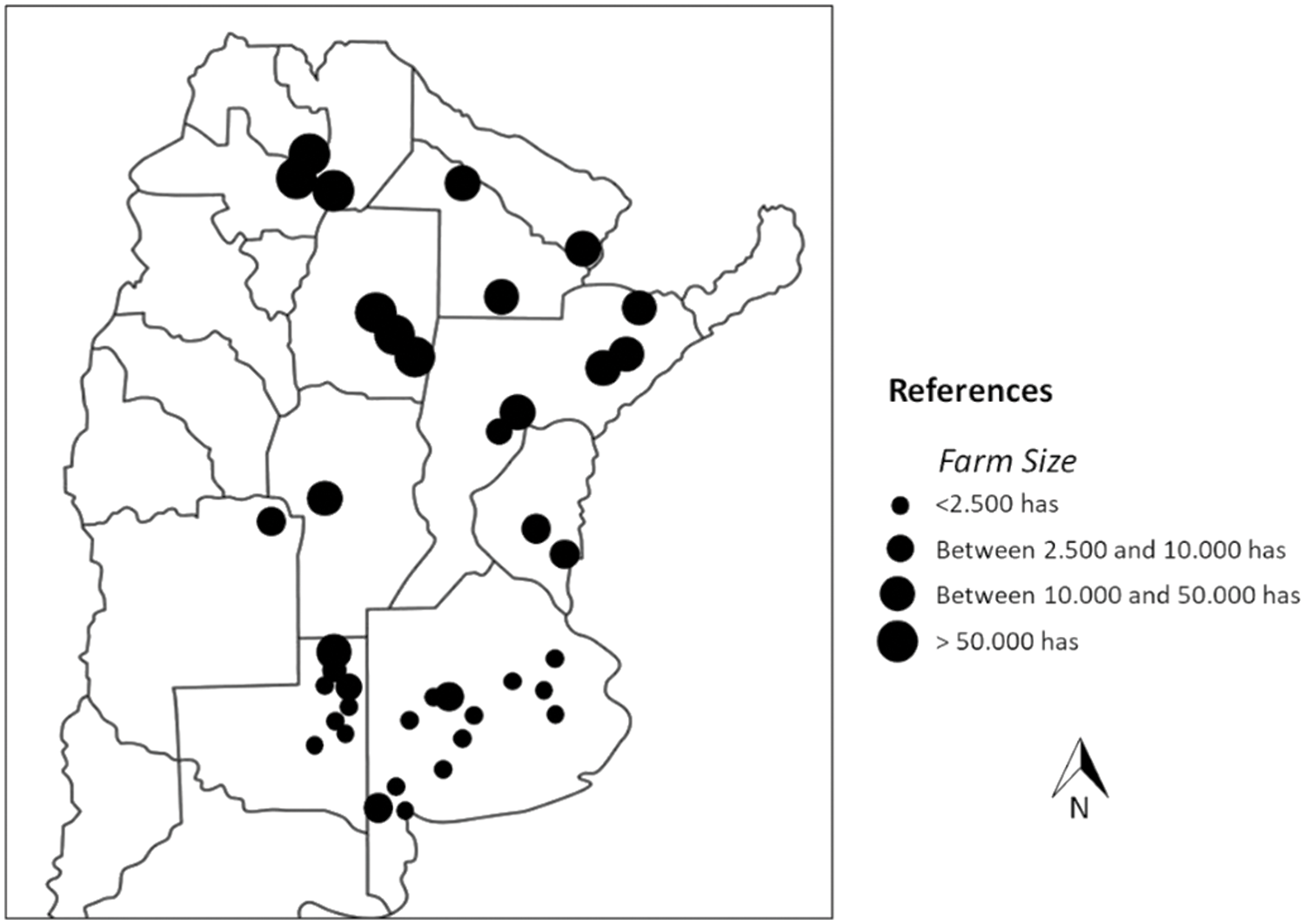
Figure 1: The geographical location in Argentina of 40 cattle-raising farms analyzed in this study

Many of the studied systems in semiarid areas, generally known as “beef production on native woodlands”, respond to some of the typologies of silvo-pastoral systems that involve extensive cattle farming with cows and steers spending part of the year in woodlands that host native grasses. Native species of the genus Erodium, Medicago, Stipa, Poa and Panicum are common and frequent in vegetation patches, especially in temperate semi-arid lands. In the open sectors of the farms, native species tend to be replaced by C4 cultivated grasses such as Gatton panic or Panicum spp. This substitution model is spreading rapidly especially in subtropical and temperate semarid lands. In order to supplement the pastoral base, some agricultural plots may be allocated to produce forage from cultivated species in the more intensive production schemes.

2.3 Comparing Approaches for Carbon Accounting

While the EF resulting from LCA expresses the impact per unit of food (t), the EB, derived from LBA, aims at quantifying the impact per unit of land (ha). Based on the International Panel on Climate Change (IPCC) [23] guidelines and default factors, we computed on annual basis both emissions and capture/storage of C.

Main emissions sources of carbon dioxide (CO2), methane (CH4) and nitrous oxide (N2O) were converted in CO2eq and then into C multiplying by a factor of 0.273, obtaining the C emitted (CE) (Eq. (1)). The study includes those emissions due to (i) changes in C stocks due to land-use change (LUC), (ii) biomass burning (fire/burning), (iii) CH4 from enteric fermentation (enteric), (iv) CH4 and N2O from manure deposited on pasture by grazing animals (manure), (v) CO2 soil management practices (Soil mng), (vi) N2O from fertilizers use (N-fert) and (vii) CO2 from fossil-fuels used in field operations (fuels). Beyond the analysis of emissions due to beef production, we included emissions from the most common annual crops of soy and maize in order to estimate the C footprint of grains used as cattle supplementary feeds.

CE=[LUC+fireburning+enteric+manure+soil mgn+N−fert+fuels]×0.273 (1)

In terms of default data/factors, we relied on different sources that included data from IPCC Tier 1 [23], FAO [4,24], Tubiello et al. [25], Allen et al. [26], Cain et al. [27], Smith et al. [28], Brander et al. [29], Colomb et al. [30] and ICSU EU [31]. In Tables S1–S5, we show the default factors that we used in this work.

We expressed production outputs in terms of kilograms of live weight leaving the farm gate in the case of beef and in terms of fresh weight in the cases of maize, soybean and wheat production. We computed the same data to account for both, emissions per unit of product (kg C t product−1) and emissions per unit of land (kg C ha−1 year−1).

Various sources [11,32–38] were used to an annual account for C captured/stored in dry matter (CDM) by above-ground (AGB) and below-ground biomass (BGB). We did not considered C stored in soil organic matter (the most stable fraction) because of uncertainty regarding reliable values. AGB and BGB were the resources (r) that we used to assess capture and store of C in woody vegetation (wbr). On the other hand, we only assessed BGB in the case of grazing resources (g) (grasslands, cultivated pastures, etc.) and crops (c) because the aerial biomass (gcbr) was the fraction consumed in the case of grazing animals, and harvested by humans in the case of annual crops. A factor = 0.47 was used to convert the dry matter of biomass into C (Eq. (2)). In Tables S1–S5, we show the default data we applied to estimate C stored by biomass in different biomes.

CDM= [∑n=1wbrAGBBGB x wbr]+ [∑n=1gcbr⁡BGB x gcbr] x 0.47 (2)

The annual CB in areas of beef production was the result of the difference between the carbon captured/stored by different biomass resources, and the carbon emitted from different sources (Eq. (3)). Expressing both in terms of t C ha−1 year−1, the net result can be positive, neutral or negative. Positive balances only involve cases in which the stored C is greater than C emitted, and thus the farm can show a C credit.

CB=CDM−CE (3)

2.4 Comparing Approaches for Water Accounting

Water use in farming is an issue of increasing global interest because the competition for freshwater between different economic and social sectors grows. Most studies generally refer to water withdrawals, but studies about evaporative water use (or water consumption) are rather scarce. We focused our research on this last issue.

Without being a mirror image, the notions of water footprint (WF) and water balance (WB) resemble the notions of CF and CB. Agricultural activities consume and pollute water. We refer here to the WF as the total water consumed and polluted by a given product throughout different stages in its food chain. The concept of WF was originally developed by Zimmer [39–41]. Based on the guidelines of the Water Footprint Network, Mekonnen et al. [42] quantified the water footprint of global crops and their derived products, such as flours, beverages, fibers and biofuels. Primary production normally occurs at a specific site, but the WF of a final product in a super-market may show spatial and temporal disconnection from water processes that occur at the farm stage. According to Hoekstra et al. [43], the global food system accounts for about 85% of global freshwater consumption.

The WF of the beef chain represents the total volume (liters (l) or cubic meters (m3)) of freshwater used, directly or indirectly, to produce one kg or ton beef. On the other hand, the WB (expressed as m3 ha−1 year−1) refers to amount of water used to produce beef at the farm stage. The WB is the difference between the amount of water consumed and the amount of water demanded by beef cattle per hectare in one year. Both indicators comprise different sources: Water may come from rain, from water body reserves or circulating water, or from polluted wastewater. The green water refers to the rainwater directly captured and transpired by plants at the farm stage. The blue water refers to the volume of surface and groundwater consumed for producing beef, milk or animal feeds. The grey water refers to the volume of freshwater that is loading pollutants.

In the case of the WF of beef (WF beef), expressed in liters per kg beef, is equal to the sum of water consumption (WC) based on WF of feeds consumed (WF feeds) plus the water drunk (WD) by different cattle categories k (cows, steers, finishing steers, bulls), and then divided by beef production P (kg) (Eq. (4)).

WF beef= ∑n=1k⁡[WF feeds+WDP] (4)

We relied on data from a publication by Frank et al. [44] based on the survey of 198 commercial farms in the Pampas of Argentina. Authors utilized an approach that assessed the water consumed by different farming activities. In the case of beef production, the two main ways of consumption were drinking water and the water used for the production of animal feeds. The notion of ‘‘water memory’’ referred to the indirect usage of water through the food (grasslands, pastures, concentrates) consumed by each animal. Despite there are factors affecting the daily consumption of drinking water by cattle, like dry matter intake, animal size, activity or environmental factors [45], a mean value of 60 liters per head−1 day−1 was adopted. In the study areas, cattle are raised under grazing conditions, and eventually, fattening steers normally stay a short period of time (less than 20% of their life cycle) in pens for intensive feeding [46]. Around 35% of the fattening steers are finished using supplements [47]. Cattle usually graze freely on cultivated pastures, rangelands, annual crop-forages and maize stubble throughout the whole year. The “water memory” of each feeding resource was estimated for each grazing resource. We expressed water used for plant growth in terms of evapotranspiration (ET0), which comprises both fractions, evaporation (E) and transpiration (T). Likewise, we estimated the water use of grazing resources and concentrate feed through default values proposed by the standards provided by the FAO-56 approach [48]. The amount of water consumed by cattle was determined through indirect equations that estimate the daily food intake (kg dry matter head−1 day−1) for different cattle categories. To calculate water consumption, we relied on the estimation of daily dry matter (DM) consumed by each cattle category (Table 1).

To estimate the “water memory” supplied by main grain-crops (soybean and maize) utilized for animal feeding, we calculated the water consumption per crop (WCCr), expressed in mm year−1 [48], by multiplying the Kc (a dimensionless factor) of each crop and its mm of evapotranspiration rate (ET) during the evaluated farming year (Eq. (5)). Based on data from Murphy et al. [49] we obtained local ET values for the study areas in Argentina. The crop coefficient (Kc), introduced by Jensen [50], corresponds to the ratio between etc., and a reference ET (ET) value that corresponds to the atmospheric evaporative demand of a pre-defined grass typology. Data on crop coefficients, which has been empirically determined for many crops, aims to incorporate into the equation the crop type, variety and development stage. Later, we adjusted WCCr values by introducing a yield relation (Y) that represents the proportional difference between actual yields from field records, and the theoretical yields provided by literature (Eq. (5)).

WCCr=∑i=13 ET x Kc x Y (5)

2.5 Accounting for Nutrients Pollution

Assessments on intensive beef cattle warn that nitrogen (N) and phosphorus (P) excretion (among other elements) are increasingly polluting water, soil and air. Most of the excreted N pollutes through volatilization, denitrification, leaching to groundwater, and runoff to surface water. On the other hand, runoff of P excretions to waterways causes eutrophication, strongly affecting the quality of water resources [51]. International assessments predict that global livestock production will increase by 115%, triggering 23% and 54% of N and P surpluses, respectively, towards year 2050 [52].

Regarding N, the prediction of pollution risk was not still well developed. Duda et al. [53] pointed out that there is no a comprehensive, universal method to assess it in response to land-use change in agricultural and non-agricultural areas. Methods to assess nitrate pollution were described by Teng et al. [54–58].

Pollution risk in relation to the amount of N and P excreted by cattle relates to several excretion factors. Excretion coefficients vary a lot with animal categories. In order to assess cross-country estimates of pollution risk, universal excretion coefficients should aim at a common methodology supported by updated statistics. It did not still occur. In practice, there are no standardized and accurate accounting methods for calculating N and P excretion coefficients per cattle category and production level. In an attempt to clarify the issue, Šebek et al. [59] compared excretion coefficients among 10 selected European countries. Regional as well as cross-country differences in N and P excretion coefficients are large and not always comparable. The authors concluded that the so-called Balance Approach tends to be the best option available to estimate N and P excretion based on country figures.

Beyond uncertainties, we estimated the pollution risk of beef cattle production by relying on the well-documented German experience that uses a Balance Approach supported by input/output measurements. The German methodology, described by DLG [60] and Haenel et al. [61], calculates excretions for a 365-day period by subtracting the mineral deposition in feces and urine from the mineral intake via feed. The following data were required for calculations: (i) N and P content of diets, (ii) feed intake levels, (iii) amount of produced animal products and (iv) N and P contents of animal products. On this basis, we estimated the percentage of excreted minerals for different cattle categories (breeding cows, suckling calves, growing heifers, fattening steers and bulls) under extensive production conditions of Argentina (Table 2).

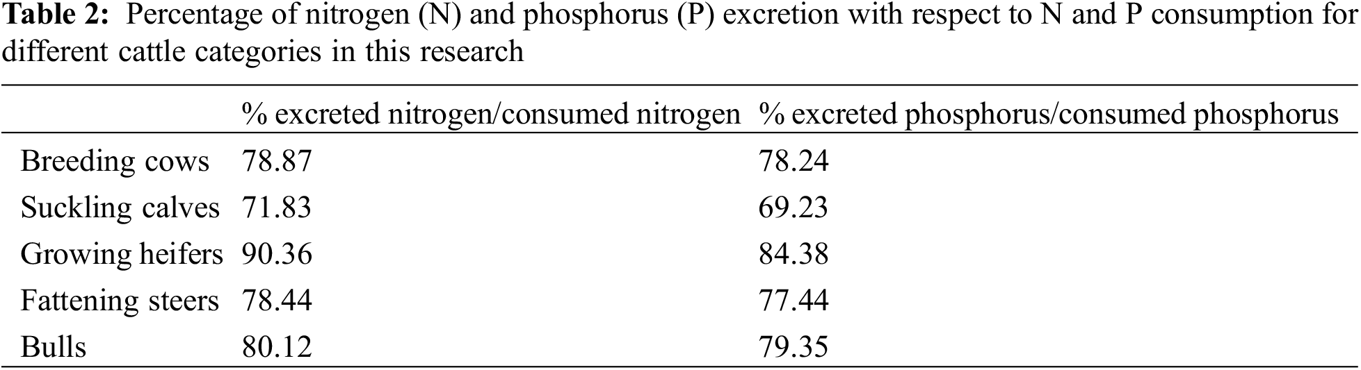
As mentioned above, we focused our study on the farm stage. In the case of beef production, expressed in kg of N or P per head per day, the calculation (Table 2 and Eq. (6)) comprised the sum of N and P consumed (C (N; P)) by each animal through feed, multiplied by the excreted N or P (Exc (N; P)) divided by 100. We estimated the consumption of N and P through the N and P density per kg dry matter of pastures and feeds that were consumed per day by each cattle category (k); N(k) represents the number of heads of each cattle category k. The factor 365 allows expressing excretions on annual basis.

PR(N;P)= ∑n=1k⁡[C(N;P) × Exc(N;P)/100 × N(k)]×365 (6)

3  Results and Discussion

The results show the environmental impact per (i) each ton of beef produced per head and (ii) per hectare of land affected to beef production. The purpose of this comparison is to evaluate which approach is the best suited to represent the environmental impacts of grazing cattle along a varying range of intensification.

In the case of carbon, the balance arises from the difference between vegetation capture/storage and emissions. In the case of water, the balance refers to the self-capacity of the system to depend exclusively on green water, or the dependency of more intense systems on supplementary water supply. As there is no a compensation mechanism to assess a balance in mineral pollution, only N and P emissions were assessed.

3.1 Characterization of Extensive Beef Production Systems in Argentina

Across the Argentine rangelands, most farmers in water-scarce regions raise beef cattle under extensive production conditions. In the most intensive cases, forage accounted for more than 80% of the feed and steers eventually received high-grain diets during a short finishing period. In our study, the maintenance of beef cattle occurred on large areas of grazing lands, which comprise a combination of native grasslands, shrublands, cultivated pastures, woody renewals and lands of sparse vegetation [11,62,63]. Worldwide, some authors consider that the extensive grazing systems play a dual role of both the beef production and the maintenance of the rural landscape [64,65].

During the last 40 years, many attempts were done to define typologies of extensive beef production systems that rely on a variety of farming views and management practices [64,66]. Since farmers in Argentina pay special attention to cattle density for handling their forage resources, quantifying stocking rates and per hectare is a suitable way to represent the notion of extensive beef production. Based on the surveyed 40 farms scattered across rangelands and pasturelands in Argentina, in Fig. 2, we show the relationships between stocking rate and per-hectare beef production. Up to certain stocking densities, the positive relationship between the number of heads per unit area and the beef production per hectare is well known. We used here the animal density as an indicator of beef cattle intensification. The lowest stocking rate and productivity per hectare correspond to the most extensive systems, and the opposite occurs as the stocking density and productivity increase. The deployment of sampled farms allows us to work on the range that varies across an extensive-intensive gradient under grazing conditions. Thus, we assumed that the most extensive beef production systems are those that fell below an annual stocking rate of one head per hectare and a beef production below 100 kg ha−1 year−1. Higher stocking rates fell within a range that varies between semi-intensive to intensive beef production systems. About 43% of analyzed data was categorized as extensive farms.

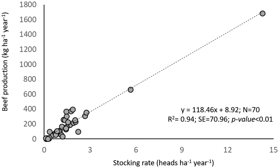
Figure 2: Relationships between stocking rate of beef cattle and annual productivity per hectare

3.2 The Environmental Footprint Per-Head

Cattle producers have continuously improved beef production efficiency in Argentina during the last 30 years by improving their breeding and management practices. The annual rate of beef production per cattle head is an important determinant of various environmental footprints [67]. Given the increasing demand for beef, cutting C emissions is a global priority. Thus, reducing the carbon footprint (CF) of beef production (expressed in kg carbon emitted per ton of beef) became an important climate mitigation strategy [68].

We found that the four evaluated footprints (C, W, and N and P pollution) tend to decline as the annual production rate per head increases (Fig. 3). In statistical terms, these environmental indicators kept in all cases a negative and significant relationship (p < 0.01) with per head beef productivity. At first sight, one may conclude that the extensive, grass-fed cattle tend to reduce their CF by consuming grasses with no intervention of feeds that demand fossil fuels for their manufacturing. On the other hand, this advantage tends be attenuated by a lower productivity rate in comparison to concentrate-fed animals. In practice, free-ranging cattle generally spend more time grazing on fields (and then emitting more C) before reaching the market [69]. In agreement with many evidences, our results show is that the CF tends to decrease as the beef production system becomes more intensive and more productive per unit of time. However, another aspect that sparks a debate deserves consideration. Most LCA methods has the limitation of setting aside the capture and storage of C in biomass and soil. As Blaustein-Rejto et al. [70] state, this gives an incomplete picture of the C economy in farming. For example, the notion of carbon footprint implies the sole consideration of carbon emissions as the only indicator of environmental impact. Under this vision, the possibility of capturing and retaining carbon in biomass and soil, as occurs in terrestrial ecosystems is set aside. Footprinting therefore offers only a partial picture of the carbon economy in the case of extensive grazing systems. To compensate for this shortcoming, here we introduced the concept of carbon balance (CB) in Section 3.4, which not only accounts for emissions losses, but also for carbon gains through captures and storage in some biophysical components of the ecosystem. In Fig. 3 and Table 3, we show the estimated footprints for C, WF and N and P pollution.

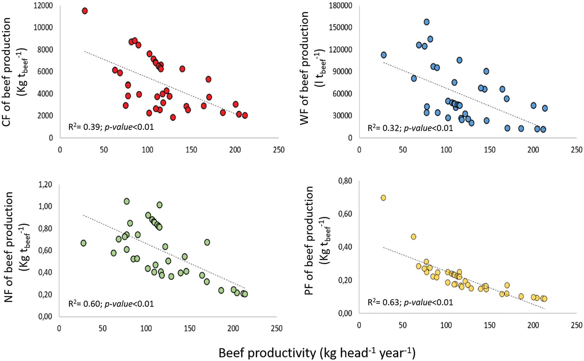
Figure 3: Relationships between per head beef productivity (kg head−1 year−1) and the environmental footprints of carbon (C), water (W), and nitrogen (N) and phosphorus (P) pollution in 40 beef production farms of Argentina

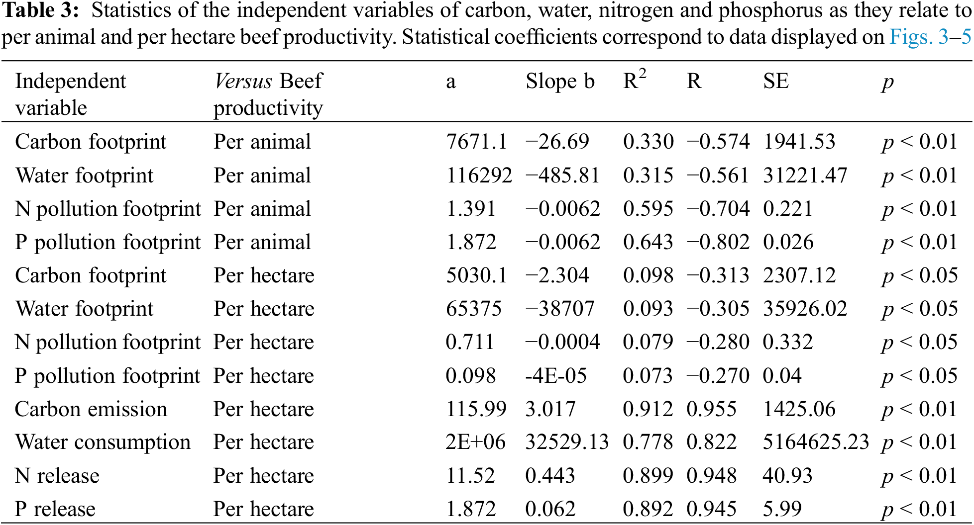
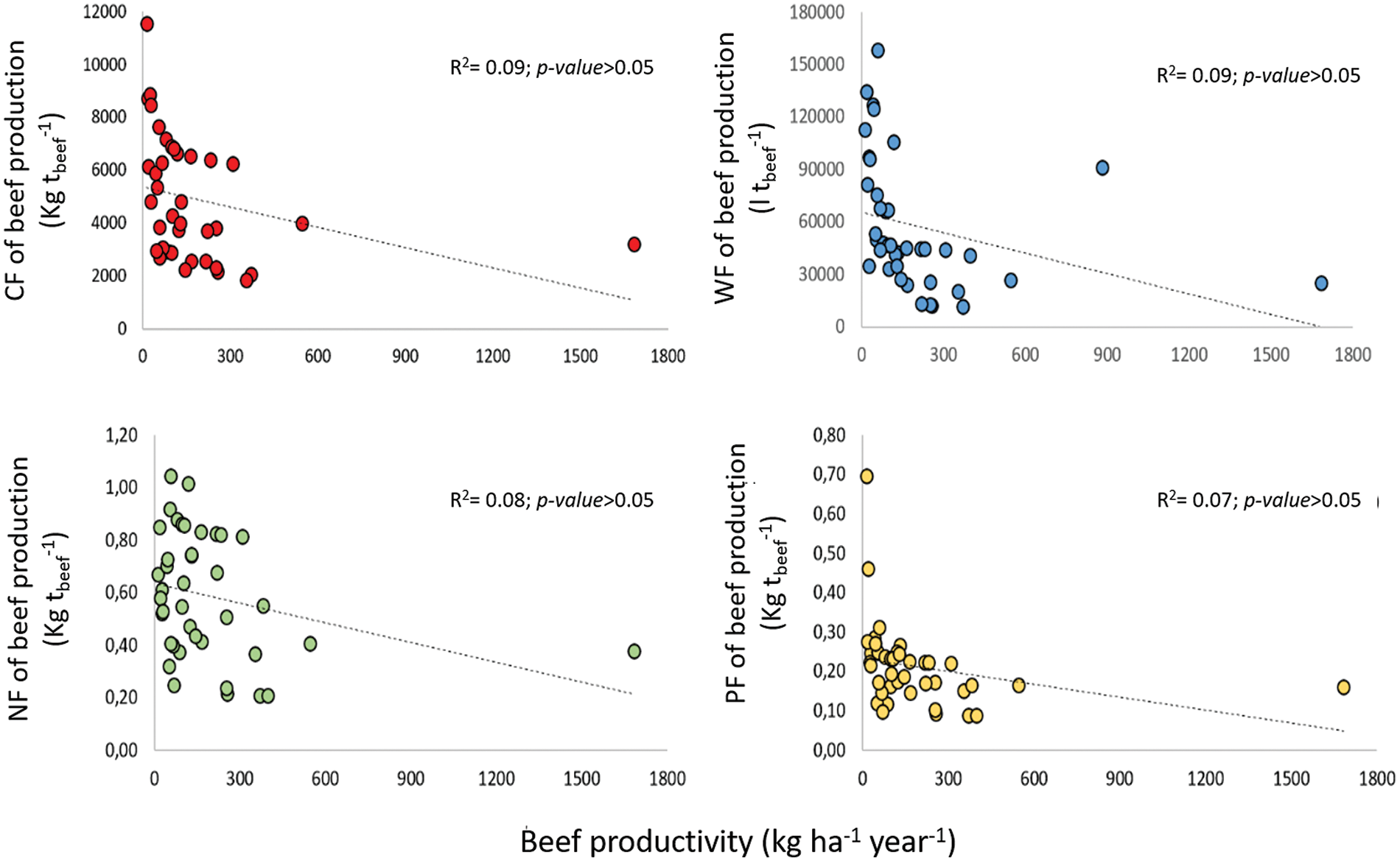
Figure 4: Relationships between per hectare beef productivity (kg ha−1year−1) and the environmental footprint of carbon, water, and nitrogen and phosphorus pollution in 40 beef-production farms of Argentina

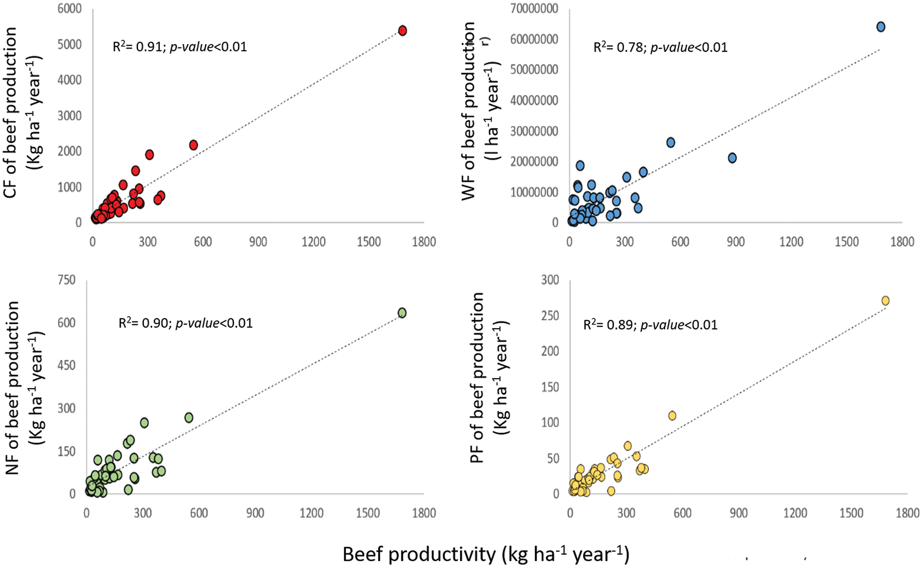
Figure 5: Relationships between per hectare beef productivity (kg head−1 year−1) and the environmental footprint of carbon, water, and nitrogen and phosphorus pollution in 40 beef-production farms of Argentina

Regarding the water footprint, the growing demand of beef due to the growth of world population has risen concerns about the pressure of beef cattle on water resources [71]. Pahlow et al. [72] have investigated impacts of intensive and extensive production systems. Cattle raised under the traditional extensive system generally utilize lands of poor soils that receive low precipitation. Those lands are generally unsuitable for cropping and breeding of non-ruminant species. Besides, extensive beef cattle systems largely depend only from scarce rainfall (green water) to persist. On the other hand, the most intensive systems usually require supplementary feeds produced elsewhere to sustain a higher beef productivity. In practice, this represents a non-material input of extra water embedded in the external feeds. In turn, this input should be added to the WF calculations. In agreement with research from Deutsch et al. [73–75], our results show that the WF tends to decrease as the intensity of beef production increases. Given that the more extensive systems utilize only green water, the competition with other sectors for extra water disappear. As Ricard [76] demonstrated, more than 90% of green water use in Argentina, Brazil, Paraguay and Uruguay occurs in lands allocated to extensive beef production.

The multiplication of pollution cases due to the release of excessive amounts of P and N to the environment are increasing cause of concern since many years ago [77,78]. In USA, for example, the estimations indicate that more than 30% of the total N and P loading to the national drinking water resources is related to livestock activities, which are a primary accelerator of global nutrient cycling [79]. Few investigations have provided enough information about the potential for nutrient pollution of extensive cattle farming in Argentina. The opposite occurs with intensive cattle farming, which is a cause of growing concern in areas where this type of livestock systems tends to increase.

In response to the method applied, our results show pollution trends that were similar to those of the CF and WF. Both, N and P emissions, tends to decrease in response to the increasing cattle head production. Despite this decreasing response, the total amount of nutrients released to the environment grows as the intensification level increases.

3.3 The Environmental Footprint Per-Hectare

Do environmental footprints maintain the same trends when evaluated per hectare instead of per animal head? If trends stayed the same, environmental footprints would be equally useful both for farmers who prioritize per capita production and for producers who favor production per hectare. We should not expect a symmetrical behavior.

When we display the environmental footprints in relation to beef productivity per hectare, we found that the relationships were not statistically significant (p > 0.05) in any case (Fig. 4 and Table 3). The notion of EF, which is valuable and useful when evaluated in terms of animal production, does not seem to be equally useful when analyzed per hectare of land. A recent research in Argentina [80] showed that the CF is insensitive to variations in the production intensity of the farm. In other terms, CF appears as a rigid method that does not detect the transition from an extensive system to a more intensive one.

This lack of relationship may confound beef producers who are accustomed to handle the hectare of land as a reference unit. A possible alternative to clarify the matter is to replace the notion of environmental footprint with the notion of environmental impact per hectare. In countries where intense beef production predominates, the notion of environmental impact per hectare is rarely used in practice. Most research generally relies on the LCA approach as universal method and the EF as a reference indicator [81,82]. However, the impact per hectare seems to be useful and necessary in areas of extensive beef production where land is a not-limiting resource [11,18,20,80].

In Fig. 5 and Table 3, results show what happened with the environmental impact per hectare when associated with the beef production per hectare. The coefficients of determination (R2) were highly significant (p < 0.01) with each of the indicators assessed.

The impact increases linearly with the level of farming intensification, and clearly the most extensive systems appear to be most friendly in environmental terms. The producers can rapidly understand the sense of this linear relationship, and even can be easily understood by consumers and social actors not strictly linked to livestock farming. This alternative insight strongly contrasts with the LCA estimates that show that EF decreases as intensification increases. Common sense indicates that both approaches are useful to interpret reality and can fruitfully be used as complementary tools to illustrate producers, consumers and policy makers.

Regarding the N and P pollution through feces and urine, there is little evidence that the accumulation of nutrients in extensive cattle farming adversely affect the surrounding environment. On the contrary, as livestock production intensifies, the long-term accumulation of N and P may become an important concern for society [83]. Based on the 40 livestock farms investigated, in Fig. 6, we display a frequency distribution of different N and P ranges of excretion. The study of the frequency distribution in the case of both nutrients allowed us to detect within which excretion ranges the most frequent impacts can occur. Both figures demonstrate that the highest frequency occurs in the lowest ranges of N and P excretion, which reveals a typical characteristic of extensive livestock systems of low animal density and low beef productivity per hectare.

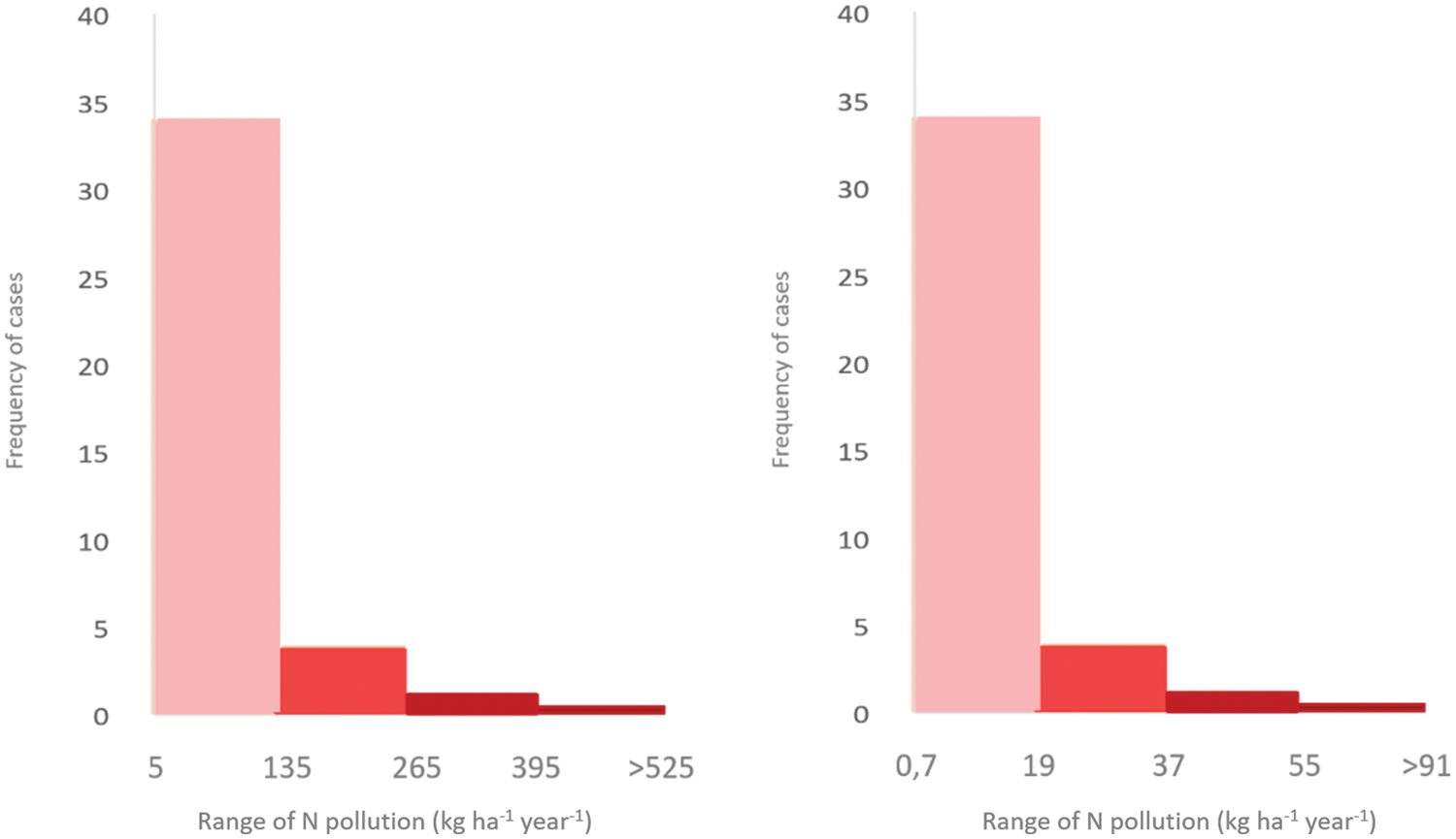
Figure 6: Estimated frequency of cases within different ranges of pollution by nitrogen and phosphorus excreted per hectare per year by cattle in 40 beef-cattle farms in Argentina

For both nutrients, almost 85% of the study farms fell within the lowest pollution range. Only a few semi-intensive and intensive farms fell within the higher pollution ranges. These results simply reflect a low risk of nutrient pollution in extensive cattle systems.

3.4 The Environmental Balance Per-Hectare

An interesting view emerged when a third dimension was incorporated into the analysis: the notion of environmental balance. The concept of balance is not generalizable to all environmental indicators since it is suitable to evaluate some of them (such as C and W) but not to others such as those of N and P pollution. In the first two cases, but not in the second ones, operate a compensation factor (e.g., C capture can offset C emission).

Due to its implication on climate change, the CB is surely the most relevant in extensive livestock farming. The CB per hectare involves both, C sources and C sinks. C sources implies all ways of emission, and C sinks are associated with plant photosynthesis. Following the conventional guidelines that IPCC Tier 1 recommends [23,36], we used default values to estimate both, the C emissions by cattle and farm operations and the C capture and store in biomass. Despite IPCC applied this procedure to forest lands, as mentioned above we extended our calculations to a variety of grazing areas that comprised grasslands, savannahs, cultivated pastures, shrublands, woodlands, woody renewals and semi-desert areas of sparse vegetation [11].

In Fig. 7, we deploy data from our analysis of CB in the 40 surveyed cattle-farms. The identification of farmers that generated C credits was quite feasible, opening a window to certify a positive CB (positive green bars). On the opposite side fell the farmers who presented a negative C balance (negative red bars). Their failed performance can be explained by deforestation of native forests and the frequent use of fire as common management practice. Farmers that can show verifiable C credits may eventually get a financial reward, a tax advantages or a public social recognition. Unlike the advantage provided by the CB, the CF would not provide the same benefit because it only estimates emissions and not C capture.

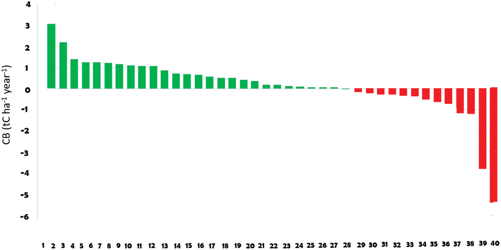
Figure 7: Estimation of the annual CB per hectare by accounting both annual carbon emission and capture in 40 beef cattle farms in Argentina. Green bars: farms showing positive balance. Red bars: farms showing negative balance

Although not strictly comparable to the CB, the WB offers a novel perspective about the use of water resources. Contrary to C, various sectors in society usually need to compete for water. Based on the method described above, the WB allows differentiating those extensive systems that only depend on green water to persist (self-sufficient), from the more intensive ones that depend on a supplementary supply of water to sustain a higher beef production level. In dependent cases, the greater productivity is supported by water embedded in supplementary feeds. Fig. 8 allows differentiating livestock systems that are self-sufficient (green bars) from those that require supplementary water (blue bars). Clearly, the most extensive livestock systems are those that show less dependence on supplementary water supplies.

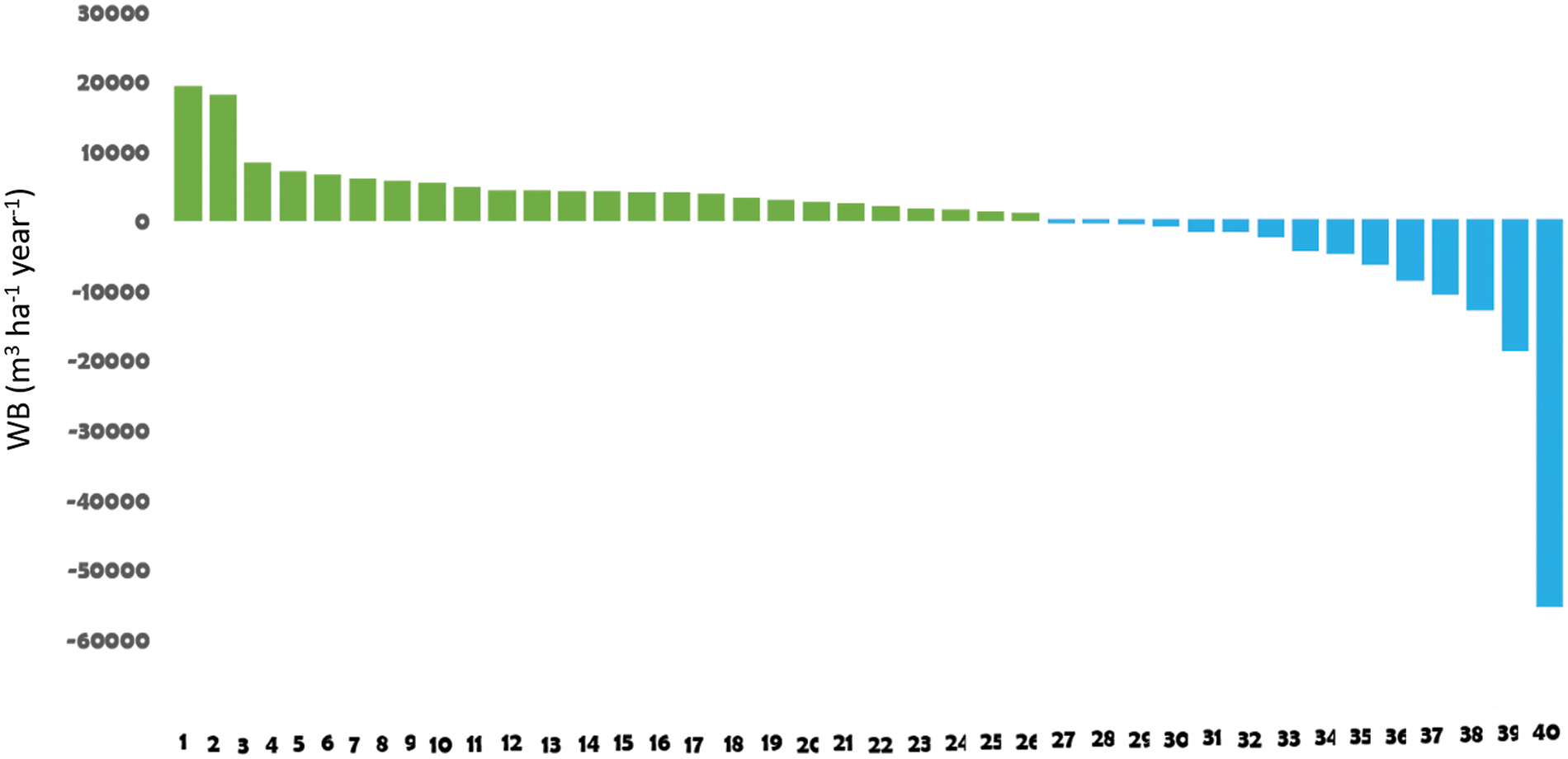
Figure 8: Estimation of the annual WB (m3 ha−1) in 40 beef cattle farms of Argentina. The balance accounted for the difference between farms that were self-sufficient in terms of pastures that only consume green water (green bars), and those that also depended on the water embedded in supplementary feeds (blue bars) produced outside the farms

3.5 Limitations of the Study and Additional Considerations

This type of studies based on the analysis of real commercial farms is limited by data availability and data quality. As we mentioned above in the methodological section, the selection of the study farms was driven by the access to reliable records. Thus we discarded farms that showed doubtful data in relation to the average values recorded in each study region. This procedure was used to reduce the degree of uncertainty regarding the information and data, assuming that some biases were inevitable in a context of practical farming.

We based our study on a limited sample of beef production farms in Argentina. Although the data reflect common farming conditions in the analyzed sites, the geographical extrapolation of results to geographically larger areas is not feasible.

Regarding analytical results, it is clear that correlation does not mean causality. Beyond the statistical significance of the relationships, other factors not considered in this study can partially explain the trends showed by our regression analyses.

4  Conclusions

Given its usefulness for informing the consumer located at the end of the food chain, the notion of Footprint allows quantifying the environmental impact of a full beef supply system. It is understandable how easy may be for a consumer in industrialized countries to interpret an impact per unit of weight of the product they are buying at the supermarket.

It may not be the same case for producers and consumers in developing societies that are located at the beginning of the beef supply chain. The notion of Footprint may not necessarily be equally useful. It is more useful to quantify the Environmental Impact per unit of land allocated to cattle farming. Even more useful if it allows differentiating the individual performance of each livestock producer. This benefit materializes if society wills to reward good management practices through tools such as C credits (valuable in the C market), tax exemptions, or simply to reward social recognition because of their transparency to in managing critical environmental variables.

The notions of CB and WB are relevant in these times in which the production and marketing of beef is associated with climate change and the use of increasingly scarce resources such as land and freshwater. Limiting land and freshwater is probably more relevant in developed countries than in developing ones. In the particular case of Argentina and other South American countries, neither land nor water is dramatically limiting the production of beef as occurs in the European Union. The availability of grazing land (especially in semi-arid regions) makes it possible to sustain extensive systems in which not only carbon emissions are relatively low, but also carbon capture and storage in biomass and soil is significant. These systems do not normally impose pressure on blue water reserves; instead, they depend almost entirely on green water use. Since land and rainfall are not limited to sustaining an extensive beef cattle system, there is no competition with other social and economic sectors for land and freshwater resources.

These differential characteristics determine that it is not equally useful to use the same ideas, concepts, and indicators to assess the environmental impact in countries of extensive cattle farming as in countries where intensive beef production predominates. Beyond differences, the dissemination of data resulting from applying both tools (Footprints and Environmental Impact) at the same time may become an important step to address a more comprehensive view of the environmental assessment and the certification of production processes.

Regarding climate change, it is essential to consider the practical implications of using different environmental indicators to address policy-and decision-making. Practical examples can support mitigation strategies and climate adaptation efforts. Both policymakers and stakeholders can get reliable information to make decisions under an increasingly unpredictable climate. Future research should focus on the refining of existing approaches and propose novel methods for improving the environmental impact assessment in extensive beef-production systems.

Acknowledgement: The authors are deeply appreciative of the academic environment and institutional backing that made this research possible.

Funding Statement: The authors received no specific funding for this study.

Author Contributions: The authors confirm contribution to the paper as follows: research design: Ernesto Viglizzo; data collection: Ernesto Viglizzo; data analysis: Florencia Ricard; analysed data interpretation: Florencia Ricard; figures and tables elaboration: Florencia Ricard; interpretation of results: Ernesto Viglizzo; writing: Ernesto Viglizzo. All authors reviewed the results and approved the final version of the manuscript.

Availability of Data and Materials: The data supporting the findings of this study are included in the supplementary material, which comprises five detailed tables containing all the indices and coefficients utilized. For further inquiries or access to additional data, readers are encouraged to contact the corresponding author.

Ethics Approval: Not applicable.

Conflicts of Interest: The authors declare that they have no conflicts of interest to report regarding the present study.

Supplementary Materials: The supplementary material is available online at https://doi.org/10.32604/phyton.2024.052513.

References

1. Sargison ND. The critical importance of planned small ruminant livestock health and production in addressing global challenges surrounding food production and poverty alleviation. N Z Vet J. 2020;68(3):136–44. doi:10.1080/00480169.2020.1719373. [Google Scholar] [PubMed] [CrossRef]

2. Henchion M, Moloney AP, Hyland J, Zimmermann J, McCarthy S. Trends for meat, milk and egg consumption for the next decades and the role played by livestock systems in the global production of proteins. Animal. 2021;15:100287. doi:10.1016/j.animal.2021.100287. [Google Scholar] [PubMed] [CrossRef]

3. Ricard MF, Mayer MA, Viglizzo EF. The impact of beef and soybean protein demand on carbon emissions in Argentina during the first two decades of the twenty-first century. Environ Sci Pollut Res. 2021;29(14):20939–46. doi:10.1007/s11356-021-16744-8. [Google Scholar] [PubMed] [CrossRef]

4. Faostat FAO. Food and agriculture data. Available from: http://www.fao.org/faostat/en/. [Accessed 2023]. [Google Scholar]

5. Steinfeld H, Gerber P, Wassenaar T, Castel V, Rosales M, de Haan C. The Livestock’s long shadow: environmental issues and options. Rome: Food and Agriculture Organization of the United Nations; 2006. [Google Scholar]

6. Poore J, Nemecek T. Reducing food’s environmental impacts through producers and consumers. Science. 2018;360(6392):987–92. doi:10.1126/science.aaq0216. [Google Scholar] [PubMed] [CrossRef]

7. Grippa M, Solazzo E, Guizzardi D, Monforti-Ferrario F, Tubiello FN, Leip AJNF. Food systems are responsible for a third of global anthropogenic GHG emissions. Nat Food. 2021;2(3):198–209. doi:10.1038/s43016-021-00225-9. [Google Scholar] [PubMed] [CrossRef]

8. Clark M, Springmann M, Rayner M. Estimating the environmental impacts of 57,000 food products. Proc Natl Acad Sci U S A. 2022;119(33):e2120584119. doi:10.1073/pnas.2120584119. [Google Scholar] [PubMed] [CrossRef]

9. Stritzler NP, Rabotnikof CM. Nutrición y Alimentación de rumiantes en la región semiárida central argentina. 1st edArgentina: EdUNLPam; 2019 (In Spanish). [Google Scholar]

10. Saxena D, Sandhwar VK. Cow farm wastes: a bioresource for sustainable development. In: Saxena D, Sandhwar VK, editors. Bio-based materials and waste for energy generation and resource management. Netherlands: Elsevier; 2023. p. 411–29. [Google Scholar]

11. Viglizzo EF, Ricard MF, Taboada MA, Vázquez-Amábile G. Reassessing the role of grazing lands in carbon-balance estimations: meta-analysis and review. Sci Total Environ. 2019;661:531–42. doi:10.1016/j.scitotenv.2019.01.130. [Google Scholar] [PubMed] [CrossRef]

12. Putman B, Rotz CA, Thoma G. A comprehensive environmental assessment of beef production and consumption in the United States. J Clean Prod. 2023;402:136766. doi:10.1016/j.jclepro.2023.136766. [Google Scholar] [CrossRef]

13. Finkbeiner M, Ackermann R, Bach V. Challenges in life cycle assessment: an overview of current gaps and research needs. In: Klöpffer W, editor. Background and future prospects in life cycle assessment. Germany: Springer; 2014. p. 207–58. [Google Scholar]

14. Clune S, Crossin E, Verghese K. Systematic review of greenhouse gas emissions for different fresh food categories. J Clean Prod. 2017;140:766–83. doi:10.1016/j.jclepro.2016.04.082. [Google Scholar] [CrossRef]

15. Camilleri AR, Larrick RP, Hossain S. Consumers underestimate the emissions associated with food but are aided by labels. Nat Clim Chang. 2019;9:53–8. [Google Scholar]

16. Hauschild MZ, Goedkoop M, Guinée J, Heijungs R, Huijbregts M, Jolliet O, et al. Identifying best existing practice for characterization modelling in life cycle impact assessment. Int J Life Cycle Assess. 2013;18:683–97. [Google Scholar]

17. Rotz CA, Asem-Hiablie S, Place S, Thoma G. Environmental footprints of beef cattle production in the United States. Agric Syst. 2019;169:1–13. [Google Scholar]

18. West TO, Marland G. Net carbon flux from agriculture: carbon emissions, carbon sequestration, crop yield, and land-use change. Biogeochemistry. 2003;63:73–83. [Google Scholar]

19. Viglizzo EF, Frank FC, Carreño LV, Jobbágy EG, Pereyra H, Clatt J, et al. Ecological and environmental footprint of 50 years of agricultural expansion in Argentina. Glob Chang Biol. 2011;17:959–73. [Google Scholar]

20. Oliveira JD, Madari BE, Carvalho MTD. Integrated farming systems for improving soil carbon balance in the southern amazon of Brazil. Reg Environ Change. 2018;18:105–16. [Google Scholar]

21. Rønning A, Brekke A. Life cycle assessment (LCA) of the building sector: strengths and weaknesses. In: Pacheco-Torgal F, Cabeza LF, Labrincha J, de Magalhães A, editors. Eco-efficient construction and building materials. United Kingdom: Woodhead Publishing; 2014. p. 63–83. [Google Scholar]

22. van der Meer K, Ignacio L. Governance, coordination and distribution along commodity value chains. Rome: FAO; 2006. p. 85–94. [Google Scholar]

23. Eggleston HS, Buendia L, Miwa K, Ngara T, Tanabe K. IPCC guidelines for national greenhouse gas inventories. Japan: Institute for Global Environmental Strategies; 2006. [Google Scholar]

24. Gerber P, Vellinga T, Opio C, Henderson B, Steinfeld H. Greenhouse gas emissions from the dairy sector: a life cycle assessment. Rome: Food and Agriculture Organization of the United Nations (FAO); 2010. [Google Scholar]

25. Tubiello FN, Biancalani R, Salvatore M, Rossi S, Conchedda GA. Worldwide assessment of greenhouse gas emissions from drained organic soils. Sustainability. 2021;8:1–13. [Google Scholar]

26. Allen MR, Shine KP, Fuglestvedt JS, Millar RJ, Cain M, Frame DJ, et al. A solution to the misrepresentations of CO2-equivalent emissions of short-lived climate pollutants under ambitious mitigation. npj Clim Atmos Sci. 2018;1:16. [Google Scholar]

27. Cain M, Lynch J, Allen MR, Fuglestvedt JS, Macey AH, Frame DJ. Improved calculation of warming-equivalent emissions for short-lived climate pollutants. npj Clim Atmos Sci. 2019;2:29. [Google Scholar] [PubMed]

28. Smith MA, Cain M, Allen MR. Further improvement of warming-equivalent emissions calculation. npj Clim Atmos Sci. 2021;4:1–3. doi:10.1038/s41612-021-00169-8. [Google Scholar] [CrossRef]

29. Brander M, Sood A, Wylie Ch, Haughton A, Lovell J. Electricity-specific emission factors for grid electricity. Ecometrica. 2011;1–22. [Google Scholar]

30. Colomb V, Amar SA, Mens CB, Gac A, Gaillard G, Koch P, et al. AGRIBALYSE®, the French LCI database for agricultural products: high quality data for producers and environmental labelling. OCL. 2014;22:D104. doi:10.1051/ocl/20140047. [Google Scholar] [CrossRef]

31. ICSU EU. ISCC EU 205. Greenhouse gas emissions, version 4.0. Brussels: European Commission; 2021. [Google Scholar]

32. Ansín OE, Oyhamburu EM, Hoffmann EA, Vecchio MC, Ferragine MC. Distribución de raíces en pastizales naturales y pasturas cultivadas de La Pampa Deprimida Bonaerense y su relación con la biomasa forrajera. Rev Fac Agron. 1998;103:141–8 (In Spanish). [Google Scholar]

33. Liebman MZ, Jarchow ME, Dietzel RN, Sundberg DN. Above-and below-ground biomass production in corn and prairie bioenergy cropping systems. In: Iowa State University Research and Demonstration Farms Progress Reports; 2014. [Google Scholar]

34. Mitsch WJ, Bernal B, Amanda M, Nahlik AM, Mander U, Anderson CJ, et al. Wetlands, carbon, and climate change. J Landsc Ecol. 2013;28:583–97. doi:10.1007/s10980-012-9758-8. [Google Scholar] [CrossRef]

35. Mónaco N, Santa V, Rosa MJ, Autran V. Evaluación de métodos indirectos para estimar biomasa en un pastizal natural del Sur de Córdoba (Argentina Central). Eur Sci J. 2017;13:1857–7881 (In Spanish). [Google Scholar]

36. Gitarskiy ML. The refinement to the 2006 IPCC guidelines for national greenhouse gas inventories. Fundam Appl Climatol. 2019;2:5–13. doi:10.21513/0207-2564-2019-2-05-13. [Google Scholar] [CrossRef]

37. Kehoe E, Salvagiotti F. Contribución de la biomasa subsuperficial de soja al índice de cosecha. Oliveros, INTA: EEA; 2020 (In Spanish). [Google Scholar]

38. Spawn SA, Sullivan CC, Lark TJ, Gibbs HK. Harmonized global maps of above and belowground biomass carbon density in the year 2010. Sci Data. 2020;7:1–22. [Google Scholar]

39. Zimmer D. Virtual water trade: proceedings of the international expert meeting on virtual water trade; 2003. Available from: https://cir.nii.ac.jp/crid/1370567187526717441. [Accessed 2024]. [Google Scholar]

40. Hoekstra AY, Chapagain A. Globalization of water: sharing the planets freshwater resources. Oxford, UK: Blackwell; 2008. p. 224. [Google Scholar]

41. Hoekstra AY, Mekonnen MM. The water footprint of humanity. Proc Natl Acad Sci U S A. 2012;109(9):3232–7. [Google Scholar] [PubMed]

42. Mekonnen MM, Hoekstra AY. National water footprint accounts: the green, blue and grey water footprint of production and consumption. In: Value of water research report series no. 50. Delft, Netherlands: UNESCO-IHE; 2011. p. 95. [Google Scholar]

43. Hoekstra AY, Chapagain AK. Water footprints of nations: water use by people as a function of their consumption pattern. In: Craswell E, Bonnell M, Bossio D, Demuth S, van de Giesen N, editors. Integrated assessment of water resources and global change: a north-south analysis. Netherlands: Springer; 2007. p. 35–48. [Google Scholar]

44. Frank FC, Viglizzo EF. Water use in rain-fed farming at different scales in the Pampas of Argentina. Agric Syst. 2012;109:35–42. [Google Scholar]

45. Eisemann JH. The 8th revised edition of the nutrient requirements of beef cattle: protein and metabolic modifiers. In: Memoria. XXVI Reunion Internacional sobre Producción de Carne y Leche en Climas Cálidos. Univ. Autónoma de Baja California. México: Instituto de Ciencias Agrícolas; 2016. p. 45–54. [Google Scholar]

46. Ministerio de Economía de Argentina. Informe de Cadenas de Valor. Ficha sectorial: ganadería y carne vacuna, Año 6, N° 59. Available from: https://www.argentina.gob.ar/sites/default/files/ficha_sectorial_carne_bovina_-_diciembre.2021.pdf. [Accessed 2021] (In Spanish). [Google Scholar]

47. INDEC. Censo Nacional Agropecuario. Dosier de principales resultados preliminares: ganadería; 2018. Available from: https://www.indec.gob.ar/ftp/cuadros/economia/dosier_cna_2018_ganaderia.pdf. [Accessed 2023]. [Google Scholar]

48. Allen RG. Crop evapotranspiration: guidelines for computing crop water requirements. FAO Irrig Drain. 1998;56:147–51. [Google Scholar]

49. Murphy GM, Hurtado RH, Fernández Long ME, Serio LA, Faroni AP, Maio S, et al. Atlas Agroclimático de la Argentina. Buenos Aires: FAUBA; 2008 (In Spanish). [Google Scholar]

50. Jensen ME. Water consumption by agricultural plants. In: Kozlowski TT, editor. Water deficits and plant growth. New York: Academic Press; 1968. vol. II, p. 1–22. [Google Scholar]

51. Sakadevan K, Nguyen ML. Livestock production and its impact on nutrient pollution and greenhouse gas emissions. Adv Agron. 2017;141:147–84. doi:10.1016/bs.agron.2016.10.002. [Google Scholar] [CrossRef]

52. Bouwman L, Goldewijk KK, Van Der Hoek KW, Beusen AHW, Van Vuuren DP, Willems J, et al. Exploring global changes in nitrogen and phosphorus cycles in agriculture induced by livestock production over the 1900–2050 period. Proc Natl Acad Sci U S A. 2013;110:20882–7. doi:10.1073/pnas.1012878108. [Google Scholar] [PubMed] [CrossRef]

53. Duda R, Zdechlik R, Kania J. Groundwater nitrate pollution risk assessment based on the potential impact of land use, nitrogen balance, and vulnerability. Environ Sci Pollut Res. 2023;58:122508–23. doi:10.1007/s11356-023-30850-9. [Google Scholar] [PubMed] [CrossRef]

54. Teng Y, Zuo R, Xiong Y, Wu J, Zhai Y, Su J, et al. Risk assessment framework for nitrate contamination in groundwater for regional management. Sci Total Environ. 2019;697:134102. doi:10.1016/j.scitotenv.2019.134102. [Google Scholar] [PubMed] [CrossRef]

55. Wu W, Liao R, Hu Y, Wang H, Liu H, Yin S, et al. Quantitative assessment of groundwater pollution risk in reclaimed water irrigation areas of northern China. Environ Pollut. 2020;261:114173. doi:10.1016/j.envpol.2020.114173. [Google Scholar] [PubMed] [CrossRef]

56. Jahromi MN, Gomeh Z, Busico G. Developing a SINTACS-based method to map groundwater multi-pollutant vulnerability using evolutionary algorithms. Environ Sci Pollut Res. 2021;28:7854–69. [Google Scholar]

57. Atoui M, Agoubi B. Assessment of groundwater vulnerability and pollution risk using AVI, SPI, and RGPI indexes: applied to southern gabes aquifer system, Tunisia. Environ Sci Pollut Res. 2022;29:50881–94. [Google Scholar]

58. Xu H, Yang X, Wang D, Hu Y, Cheng Z, Shi Y, et al. Multivariate and spatio-temporal ground-water pollution risk assessment: a new long-time serial groundwater environmental impact assessment system. Environ Pollut. 2023;317:120621. [Google Scholar] [PubMed]

59. Šebek LB, Bikker P, Vuuren AM, Krimpen M. Nitrogen and phosphorous excretion factors of livestock. Task 2: in-depth analyses of selected country reports. Wageningen: UR Livestock Research; 2014. [Google Scholar]

60. DLG. Update brochures to adjust the methodology or to add other animal categories to the listing. Available from: http://www.dlg.org/fachinfos-naehrstoffausscheidung.html. [Accessed 2009]. [Google Scholar]

61. Haenel HD, Rösemann C, Dämmgen U, Poddey E, Freibauer A, Döhler H, et al. Calculations of gaseous and particulate emissions from German agriculture 1990–2010: report on methods and data (RMD). Germany: Johann Heinrich Von Thünen-Institut; 2012. [Google Scholar]

62. Viglizzo EF. Huella de carbono e intensificación sustentable en la región de Argentina, Brasil, Paraguay y Uruguay. Grupo Países Productores del Sur (GPS). Available from: https://grupogpps.org/huella-de-carbono-e-intensificacion-sustentable-en-la-region-de-argentina-brasil-paraguay-y-uruguay-por-ernesto-f-viglizzo/. [Accessed 2014] (In Spanish). [Google Scholar]

63. Jaurena M, Lezama F, Salvo L, Cardozo G, Ayala W, Terra J, et al. The dilemma of improving native grasslands by overseeding legumes: production intensification or diversity conservation. Rangeland Ecol Manag. 2016;69(1):35–42. [Google Scholar]

64. Morgan-Davies C, Waterhouse A, Wilson R. Characterisation of farmers’ responses to policy reforms in Scottish hill farming areas. Small Ruminant Res. 2012;102:96–107. [Google Scholar]

65. McAllister TA, Stanford K, Chaves AV, Evans PR, de Souza Figueiredo EE, Ribeiro G. Nutrition, feeding and management of beef cattle in intensive and extensive production systems. In: Bazer FW, Lamb GC, Wu G, editors. Animal agriculture. USA: Academic Press; 2020. p. 75–98. [Google Scholar]

66. Norton LR, Bruce A, Chapman P. Identifying levers for change in UK grazing livestock systems. Front Food Syst. Available from: https://www.frontiersin.org/articles/10.3389/fsufs.2024.1366204/full. [Accessed 2024]. [Google Scholar]

67. Ogino A, Sommart K, Subepang S, Mitsumori M, Hayashi K, Yamashita T, et al. Environmental impacts of extensive and intensive beef production systems in Thailand evaluated by life cycle assessment. J Clean Prod. 2015;112(1):22–31. [Google Scholar]

68. Swain M, Blomqvist L, McNamara J, Ripple WJ. Reducing the environmental impact of global diets. Sci Total Environ. 2018;610-611:1207–9. [Google Scholar] [PubMed]

69. Capper JL. Replacing rose-tinted spectacles with a high-powered microscope: the historical versus modern carbon footprint of animal agriculture. Animal Front. 2011;1:26–32. [Google Scholar]

70. Blaustein-Rejto D, Soltis N, Blomqvist L. Carbon opportunity cost increases carbon footprint advantage of grain-finished beef. PLoS One. 2023;18(12):e0295035. [Google Scholar] [PubMed]

71. Chapagain AK, Hoekstra AY. Water footprint of nations, The Netherlands: UNESCO-IHE; 2004. vol. 1. [Google Scholar]

72. Pahlow M, Snowball J, Fraser G. Water footprint assessment to inform water management and policy making in South Africa. Water SA. 2015;41:300–13. [Google Scholar]

73. Deutsch L, Falkenmark M, Gordon L, Rockström J, Folke C. Water-mediated ecological consequences of intensification and expansion of livestock production. In: Steinfeld H, Mooney HA, Schneider F, Neville LE, editors. Livestock in a changing landscape. USA: Island Press; 2010. p. 97–111. [Google Scholar]

74. Vanham D, Bidoglio G. A review on the indicator water footprint for the EU28. Ecol Indic. 2013;26:61–75. [Google Scholar]

75. Atzori AS, Canalis C, Fransesconi AHD, Pulina GA. Preliminary study on a new approach to estimate water resource allocation: the net water footprint applied to animal products. Agric Agric Sci Procedia. 2016;8:50–7. [Google Scholar]

76. Ricard MF. Uso Sostenible del Agua en la Agricultura del MERCOSUR. Grupo GPS (Grupo de Países Productores del Sur). Available from: https://grupogpps.org/uso-sostenible-del-agua-en-la-agricultura-del-mercosur/. [Accessed 2021] (In Spanish). [Google Scholar]

77. Tam MKC, Ferrer Marti I, Loo SCJ. Combating threats to water, air and soil, our precious natural resources. ACS Sustainable Chem Eng. 2023;11:15503–5. [Google Scholar]

78. Kraham SJ. Environmental impacts of industrial livestock production. In: Steier G, Patel K, editors. International farm animal, wildlife and food safety law. Cham: Springer; 2017. p. 3–40. [Google Scholar]

79. Bouwman AF, Beusen AH, Billen G. Human alteration of the global nitrogen and phosphorus soil balances for the period 1970–2050. Global Biogeochem Cycles. 2009;23(4):1–16. doi:10.1029/2009GB003576. [Google Scholar] [CrossRef]

80. Viglizzo EF, Ricard MF. Carbon accounting per unit of food and unit of land in food production systems of Argentina. UJCR. 2023;1(2):23–33. [Google Scholar]

81. De Vries M, Van Middelaar CE, De Boer IJM. Comparing environmental impacts of beef production systems: a review of life cycle assessments. Livest Sci. 2015;178:279–88. [Google Scholar]

82. O’Brien D, Markiewicz-Keszycka M, Herron J. Environmental impact of grass-based cattle farms: a life cycle assessment of nature-based diversification scenarios. Resour Environ Sust. 2023;14:100126. [Google Scholar]

83. McAllister T. Environmental footprint of beef cattle production. Beef Cattle Research Council, Canada, Available from: https://www.beefresearch.ca/topics/environmental-footprint-of-beef-production/. [Accessed 2019]. [Google Scholar]