Sentinel-2 Satellite Imagery Application to Monitor Soil Salinity and Calcium Carbonate Contents in Agricultural Fields

1  Introduction

Soil salinity is one of the limiting factors of soil, that can be leads to soil degradation and some negative effects on crop yield in arid and semiarid areas [1] and has serious negative impacts on several aspects of agriculture and environmental sustainability [2]. Due to the high evaporative demand in these areas with limited water resources, salts tend to build up in the soil profile. This increases osmotic stress, which affects soil water availability and root water uptake while also possibly fostering the development of ion toxicities and disparities in plants. When soil salinity exceeds a predetermined tolerance threshold, crop development, transpiration rates, and yields are therefore lowered, and greater levels ultimately result in crop failure [3]. High sodium saturation of the soil exchange complex may also have additional effects on the stability of the soil’s structure and its ability to retain water. This will cause soil colloids to disperse, which will change how water and air move through the soil, reducing soil infiltration, favoring water stagnation, and possibly resulting in anoxic rootzone conditions [4]. According to the most accurate estimates, either natural processes (rock weathering, sea water infiltration into marine sediments, and atmospheric deposition) or human-induced processes (poor irrigation water management and overuse of saline groundwater resources) are responsible for the 412 million ha affected by salinity and the 618 million ha affected by sodicity [5]. These estimations, however, are known to be dependent on expert opinion from certain nations or locations rather than on precise measurements of the level of soil salinity and sodicity [6]. In order to quickly, non-invasively, and economically assess the spatial and temporal distribution of salt impacted areas on a broad scale, the scientific community has spent a lot of time and money on this over the past few decades [7]. To avoid the degradation process of agricultural land, it is important to monitor and manage the land resources, i.e., mapping of soil salt plays an important role for sustainable agricultural planning [8]. However, the accurate monitoring of soil salinity on a large-scale area is considered as one of the important factors that could avoid these problems [9]. Early efforts on the development of remote sensing technologies concentrated on assessing salinity at or near the soil surface based on the differing reflectance characteristics of salt crusts when compared with non-salt impacted soils [10].

Soil calcium carbonate (CaCO3) is considered as one of the soil properties associated with plant growth, such as soil water holding capacity and the availability of nutrients for plants [11]. Most carbonate minerals found in soils of arid regions of Sudan are calcite (CaCO3) and dolomite (Ca, Mg, CO3) minerals and exist mainly in the soils of the northern Sudan [12]. Conventional methods used for the estimation of soil properties (collection and analysis of soil samples) are laborious, time-consuming, and expensive, and may not reflect its accurate estimates [13]. For example, in terms of assessing soil salinity and CaCO3, the conventional methods show its weakness and difficulties to be implemented on large areas; this could lead to some limitation in soil management [8]. Nowadays, remote sensing methods have been demonstrated to serve as promising means to significantly increase the number of sites offering quantitative estimations of topsoil properties (e.g., soil organic carbon, pH, cation exchange capacity, texture class, EC and calcium carbonate) [14,15]. Recently remote sensing technology has become one of the varied soil monitoring methods that has become increasingly used, providing an efficient cost-effective mean to assess soil properties [9]. Diek et al. [16] reported that several methods for generating bare soil images from historical collections of satellite images from one satellite have been developed, such as the barest pixel composite. Currently a free and permanent supply of remote sensing images from Landsat-8 and Sentinel-2 (S2A) have great potential for generating high resolution information for various purposes, such as agriculture fields [17]. However, remote sensing data have been an instrumental powerful tool over conventional techniques in providing long-term timespan data images for environmental and natural resources monitoring and management at different spatial scales [9].

Many researches have been conducted to study the relationship between multiple satellite data and soil salinity and soil calcium carbonate. Lobell et al. [18] used Moderate Resolution Imaging Spectroradiometer (MODIS) data for regional-scale soil salinity assessment and reduced the effect of temporally dynamic factors using the mean of the enhanced vegetation index (EVI). Guo et al. [19] used Landsat 8 data to construct vegetation indices-salinity indices feature spaces based on the information of bare soil and vegetation; results showed that these indices can greatly improve the periodical monitoring of soil salinity. Safanelli et al. [20] estimated soil CaCO3 from two bare soil composites of 30 m resolution Landsat images with an R2 value of 0.44. Sentinel-2 has high temporal and spatial resolution, which enable more detailed and higher-frequency monitoring for practical applications [9].

Linear and quadratic regression models explain the robustness of regression approach after streamlining the outliers. The evaluation of the estimated regression equations based on the R2 metric indicates that they constitute a useful, reliable, and valuable tool for managing, describing, and predicting the soil parameters [21]. Davis et al. [22] discovered that Sentinel-2 had great potential for estimating soil properties. However, Sentinel-2 used in this study for prediction soil EC and CaCO3. As the prediction accuracy of models depends on local conditions, the present study was aimed to characterize the soil electrical conductivity (EC) and soil calcium carbonate (CaCO3) using “free-of-cost” remotely sensed images (Sentinel-2). Commonly used linear regression models were employed to link the spectral data of the topsoil (i.e., 15 cm). The specific objectives were: (i) to assess the relationship between laboratory estimated soil EC & soil CaCO3 and remotely sensed data acquired from by Sentinel-2 satellite, (ii) to develop linear regression models for the prediction of soil EC & soil CaCO3 contents in agricultural soils.

2  Materials and Methods

2.1 Study Area

The study was conducted in selected agricultural fields in in Al-Kafaa commercial farm of Al-Rajhi International Investment Company, located in the Northern region of Sudan between the latitudes of 18°10′8.503″ and 18°11′37.837″ N and the longitudes of 34°0′26.021″ and 34°11′18.415″ E (Fig. 1). Two agricultural fields (ID: S1-1, S1-2) have been selected for the study, with a total area of each field was 30 hectares and irrigated through center pivot system. The topography of the study fields was almost flat with slight undulations where the elevation ranged from 283 to 409 m. The soil in the experimental farm is mainly characterized between sandy loam to loamy sand. The major crops cultivated on the farm were wheat, alfalfa, Rhodes grass and corn. Weather in the farm was very hot in the summer (44°C ± 2°C) and cold to moderate in the spring (16°C ± 2°C) with an annual rainfall of about 37 mm.

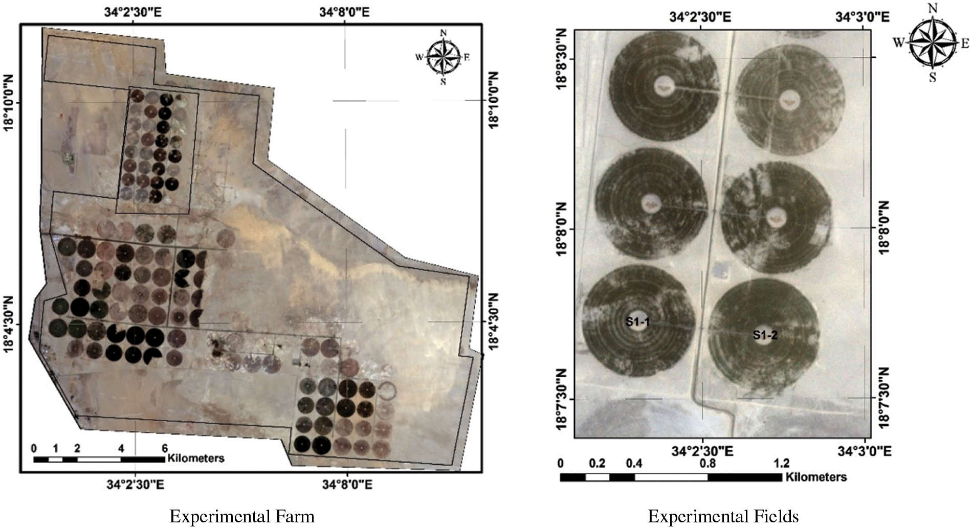
Figure 1: Location of the study area

2.2 Soil Sampling

A field survey was carried out on 25 April 2018 for a total of 72 combined soil samples from two fields were collected from the topsoil layer (0 to 15 cm). A hand-held Garmin GPS (3.8 m accuracy) was used to locate the pre-defined sampling points. The soil samples were collected using a systematic grid sampling approach with grids of 100 m × 100 m following the sampling strategy described by [23]. Subsequently, the collected soil samples were air-dried and sieved (<2 mm) to remove plant debris and large root matter. Thereafter, analyzed in the laboratory for soil pH, electrical conductivity (EC), organic matter (OM), calcium carbonate (CaCO3), as defined by Soil Survey Staff 1999. The vegetation indices generated from the satellite images were utilized to develop correlation mathematical models for prediction soil properties.

2.3 Satellite Data and Image Analysis

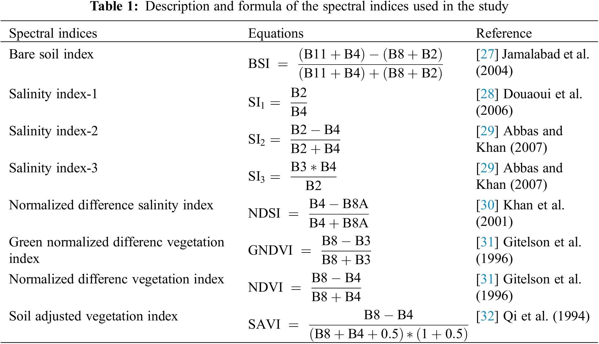
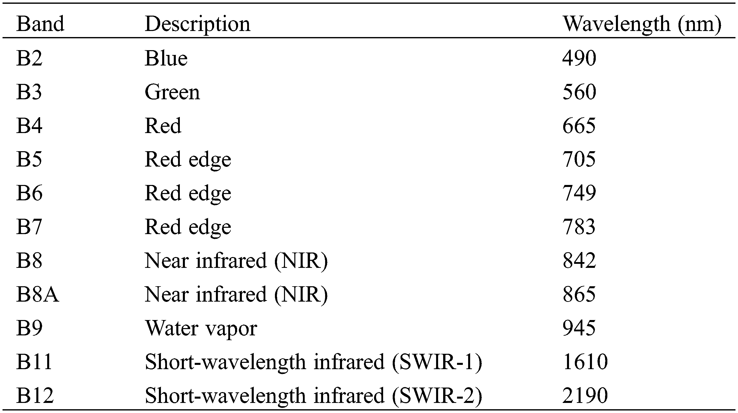
A total of two cloud-free images of Sentinel-2 (10 m × 10 m pixel size) were downloaded from the USGS portal (https://earthexplorer.usgs.gov/) corresponding to the field inventory of soil sample collection, images acquired on 28 April 2018, which was basically synchronous with the sampling time and there was no cloud in the study area. Whereas, Loiseau et al. [24] indicated that Sentinel-2 has advantages for soil monitoring because of its high spatial resolution, multispectral bands, and short revisit time. Five indices out widely used spectral indices [9] have been selected, including bare soil index (BSI), salinity index (SI1, SI2, SI3), in addition to the normalized difference salinity index (NDSI) proposed by [25], and used for the prediction of soil properties, GNDVI (Green normalized difference vegetation index), NDVI (Normalized difference vegetation index), SAVI (Soil adjusted vegetation index) As, Allbed et al. [26] reported that Normalized Differential Salinity Index (NDSI) and Salinity Index (SI) provided optimum results compared to the other indices investigated for estimating soil salinity. Description and relevant formula of the spectral indices used in the study is provided in Table 1.

2.4 Modelling and Prediction of Soil Properties

To predicted soil properties of the study fields, a regression analysis based empirical equation was generated with the Sentinel-2 against the soil properties. During the process, the relationship between the spectral reflectance of the Sentinel-2 dataset and the soil properties was assessed using the SPSS (Ver. 20) statistics software program (IBM, New York, USA). Of the collected samples, approximately 60% of observations was used to produce the regression model (i.e., calibration data) and 40% of observations was used to cross-validate the model (i.e., validation data).

2.5 Validation of Analysis

The prediction accuracy was evaluated employing the analysis of variance (ANOVA) statistics to test the strength of the developed models through the coefficient of determination (R2), mean square, the histograms of the residuals and the normal probability plots, the root mean square error (RMSE), as shown in Eq. (1), R2 validation, as shown in Eq. (2) and the standard error of the estimate (std. Error). The model with the lowest RMSE, std. Error and highest R2 values were considered to be the most applicable or ideal model [33].

RMSE =∑i=1n⁡(yi−y^i)2n (1)

R2 validation=1− ∑i=1n(yi_y^i)2 ∑i=1n(yi−y−)2 (2)

where, yi is the measured values, ŷi is the predicted values, y¯ is overall mean values and n is the amount of soil samples.

3  Results

3.1 Soil Samples Properties

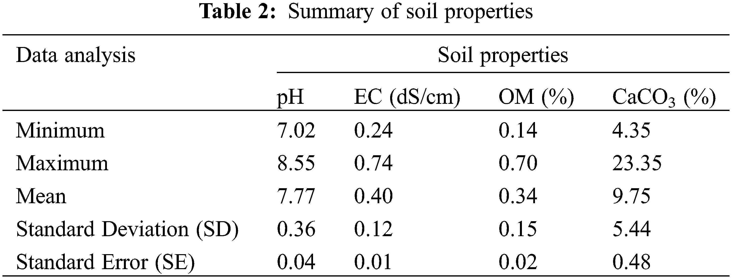
The descriptive statistics of the physicochemical parameters measured in soil samples is shown in Table 2. The soil textures classes of the studied area were mainly of loamy sand (38%), sandy loam (35%), silt loam (15%) and loamy (12%). The soil of the studied area had an EC ranging between 0.24 and 0.74 dS/cm, and pH values ranging between 7.02 and 8.55. Organic matter was very low (ranging between 0.14% 0.70%), this due to the climate is hot, however the soil contains low organic carbon. While soil CaCO3 ranging between 4.35% and 23.35% and most of the high CaCO3 values were observed at the border of field.

3.2 Performance of Soil EC Prediction Models

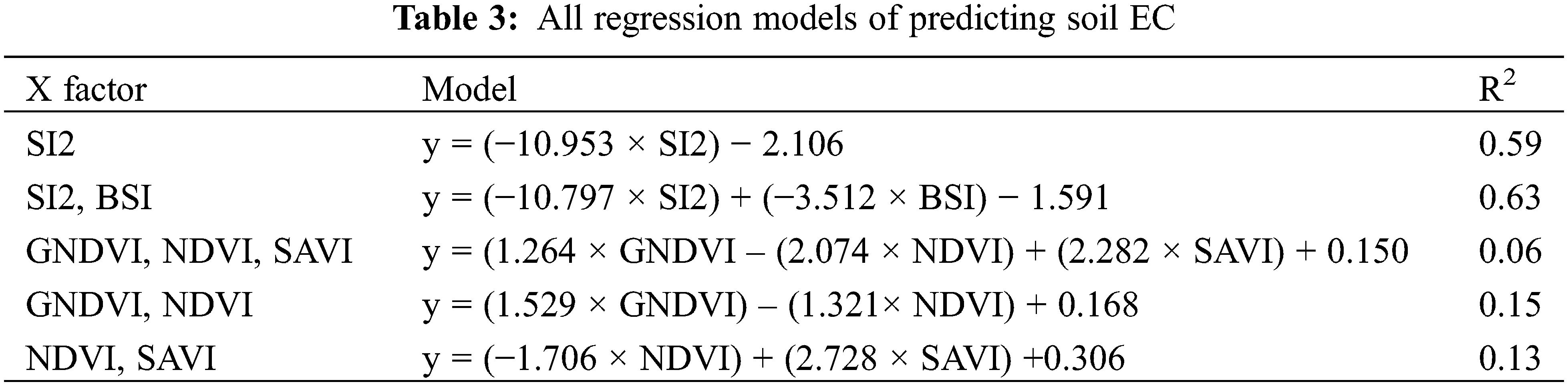
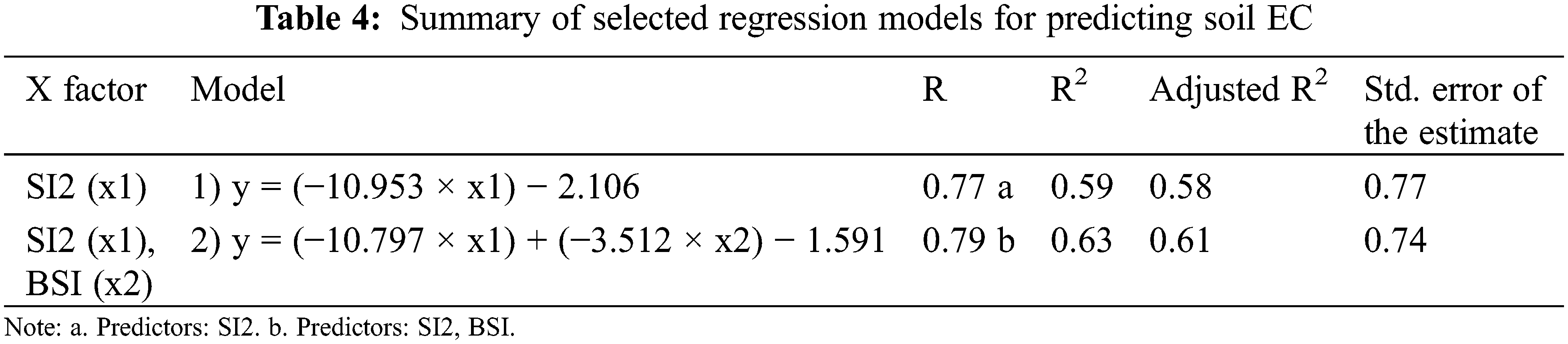
The performance of the generated soil EC models was statistically assessed. Out of studied five soil indices generated from Sentinel-2 image (Table 3), two soil indices (SI2 & BSI) showed a significant correlation with the soil EC, however, the SI2 and the BSI were found to be more suitable for predicting soil EC. The results of the soil EC and the soil indices (SI2 & BSI) were subjected to a linear regression modeling performed using the IBM SPSS statistics software program. Linear regression results (Table 4) showed two models with a significant correlation between the measured soil EC and predicted soil EC by soil indices (R2 values ranging between 0.59 and 0.63, respectively).

The ANOVA results (Table 5) also confirmed the significant relationship between the soil indices and soil EC for the two models. The accuracy of the models was performed, as shown in Table 6 and Fig. 2. The validation R2 value of Model-1 (SI2) was 0.48, which was slightly higher than the validation R2 value (0.47) of Model-2 (SI2 & BSI) and confirmed by the RMSE value of 1.32% for Model-1, which was lower than the RMSE value of 6.42% for Model-2. The regression strength of the two prediction models of soil EC was performed through the histogram analysis, the normal probability plot and the residual analysis as shown in Fig. 3. The scatter plot (Fig. 4) illustrates the validation EC data points against the corresponding measured values with an RMSE value of 1.34%.

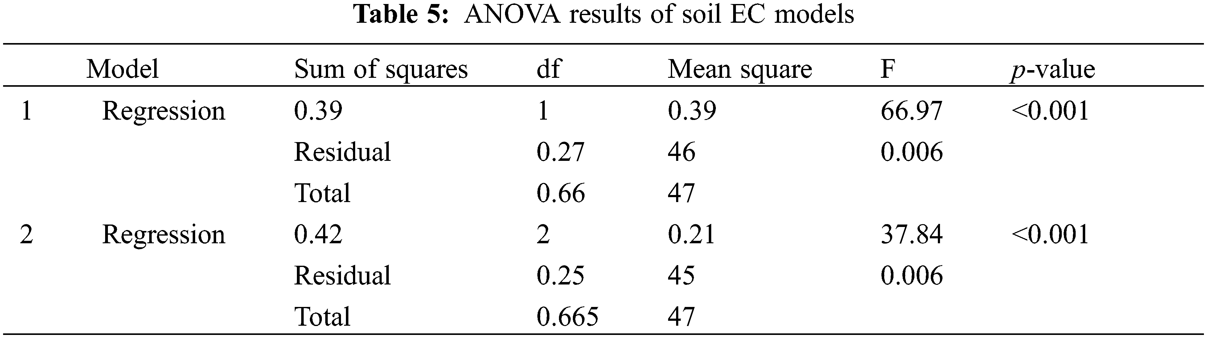
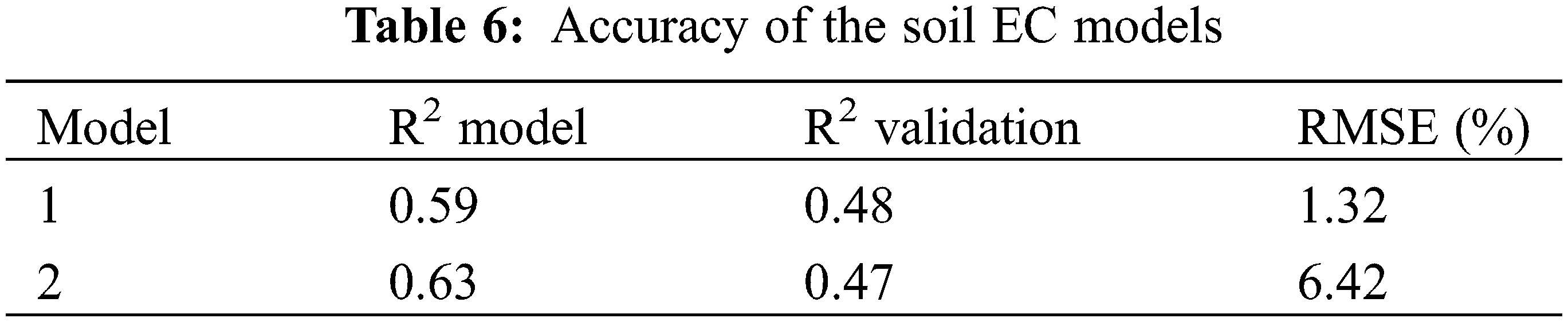
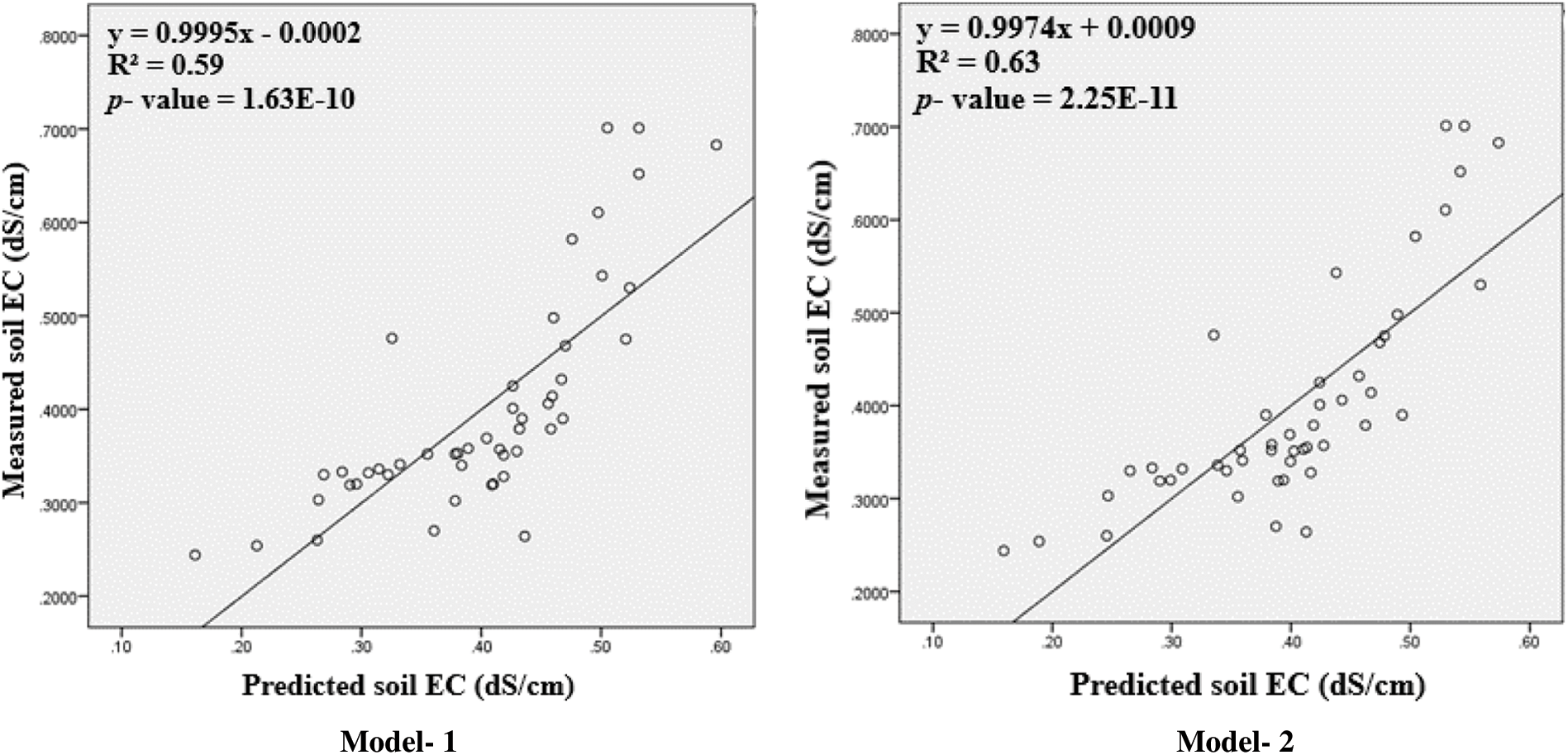
Figure 2: Relationship between the measured and predicted soil EC

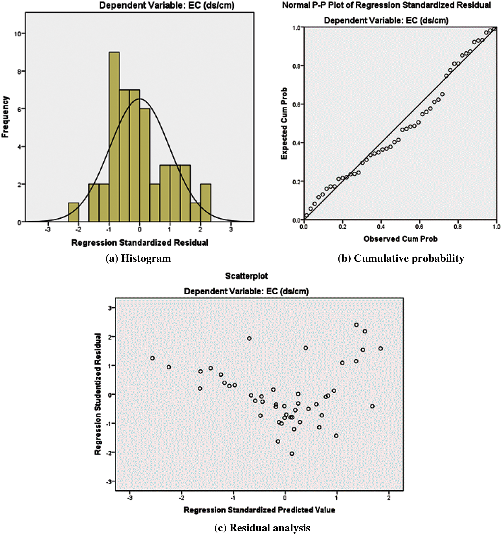
Figure 3: Histogram, cumulative probability, and residual analysis for the prediction models of soil EC

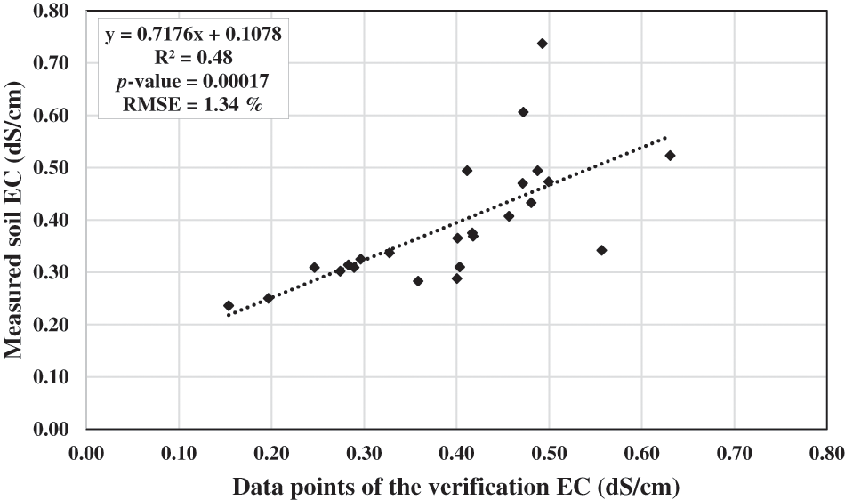
Figure 4: The validation EC data points vs. corresponding measured values

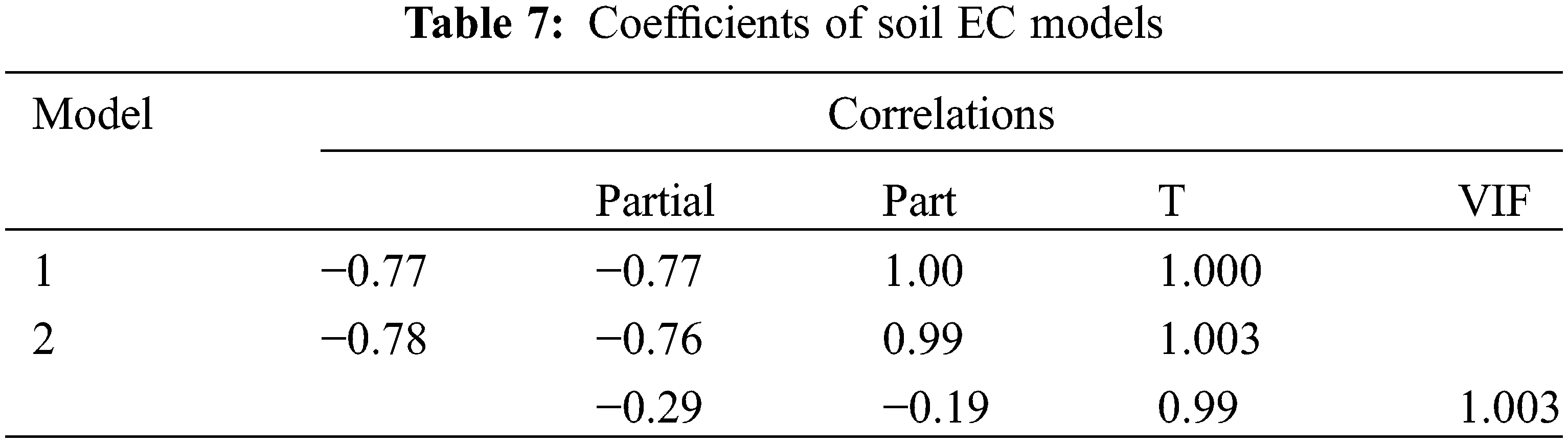
Based on the coefficients analysis including a Tolerance (T) value of 1.000 and a Variance Inflation Factor (VIF) of 1.000 (Table 7). However, Model-1 showed the most valid correlation between the measured and predicted soil EC.

3.3 Performance of Soil CaCO3 Prediction Models

The performance of the generated soil CaCO3 models was statistically assessed. Out of studied five soil indices generated from Sentinel-2 image (Table 8), wo soil indices (BSI & NDSI) showed a significant correlation between the soil indices and the soil CaCO3, however, the BSI and NDSI were found to be more suitable for predicting soil CaCO3.

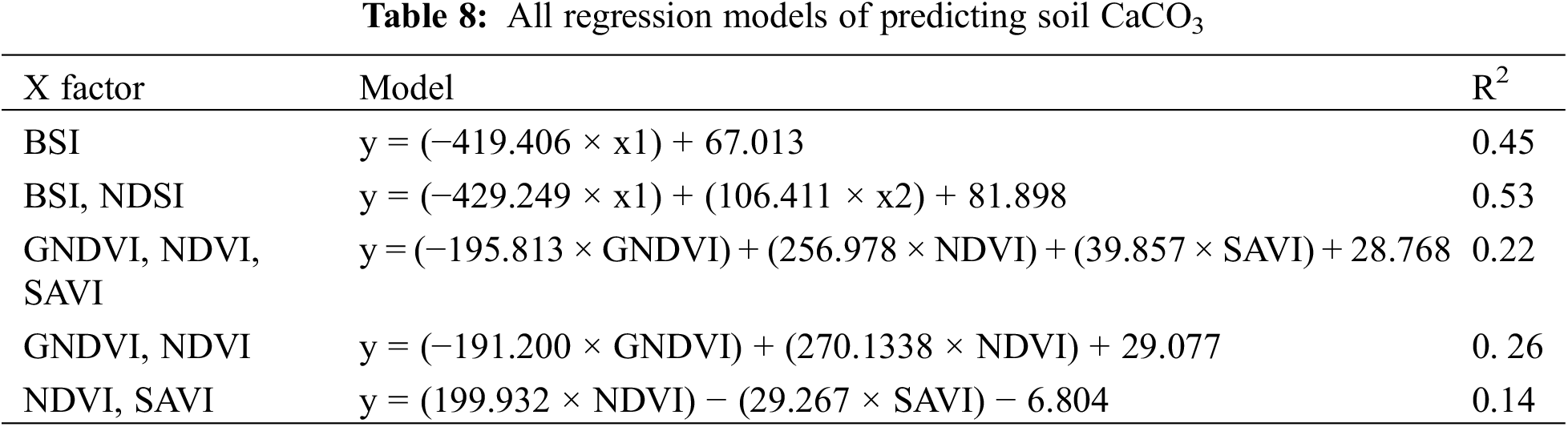
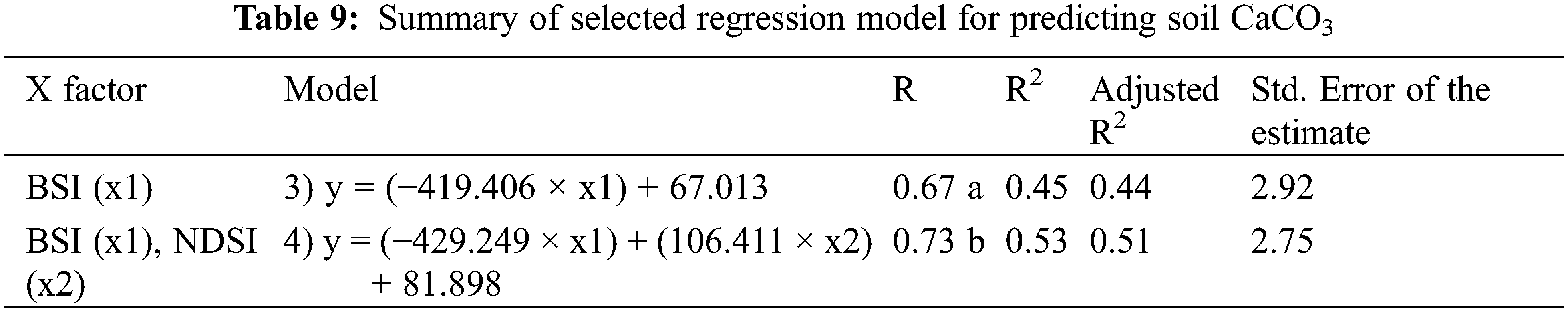
The results of the soil CaCO3 and the soil indices generated from satellite image (BSI & NDSI) were subjected to a linear regression modeling performed using the IBM SPSS statistics software program. Linear regression results (Table 9) showed two models with a significant correlation between the measured and predicted soil CaCO3 by soil indices (R2 values ranging between 0.45 and 0.53, respectively).

The ANOVA results (Table 10) also confirmed the significant relationship between the soil indices and soil CaCO3 for the two models. The accuracy of the models was performed, as shown in Table 11 and Fig. 5. The validation R2 value of Model-3 was 0.47 (BSI), which was higher than the validation R2 value (0.35) of Model-4 (BSI & NDSI) and confirmed by the RMSE value of 1.29% for Model-3 which was lower than the RMSE value of 1.55% for Model-4. The regression strength of the two prediction models of soil CaCO3 was performed through the histogram analysis, the normal probability plot and the residual analysis as shown in Fig. 6. The scatter plot (Fig. 7) illustrates the validation CaCO3 data points against the corresponding measured values with an RMSE value of 1.93%.

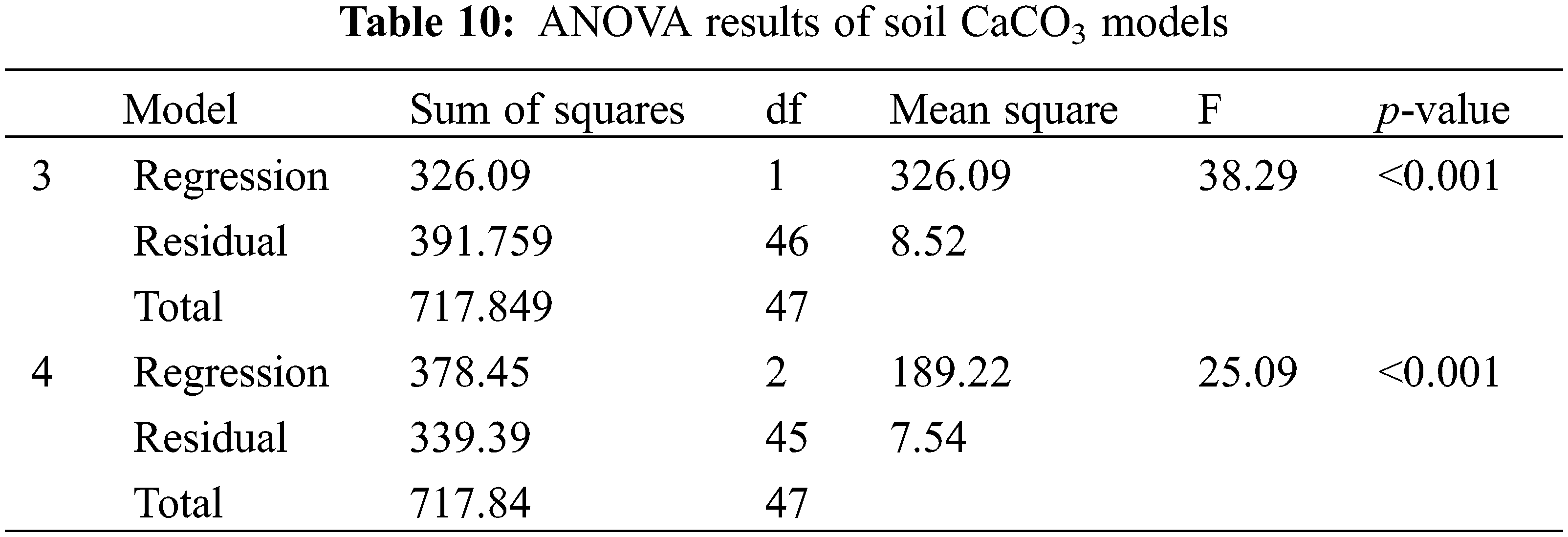
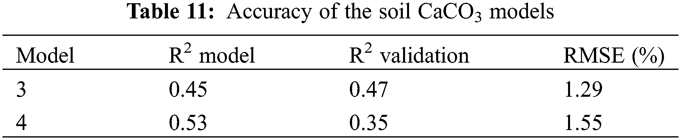
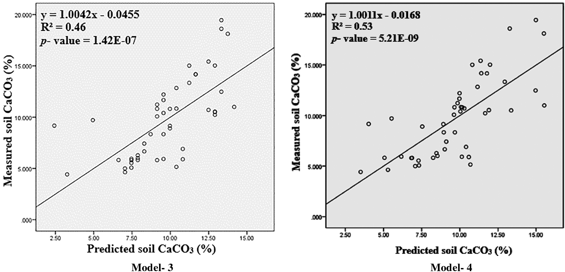
Figure 5: Relationship between the measured and predicted soil CaCO3

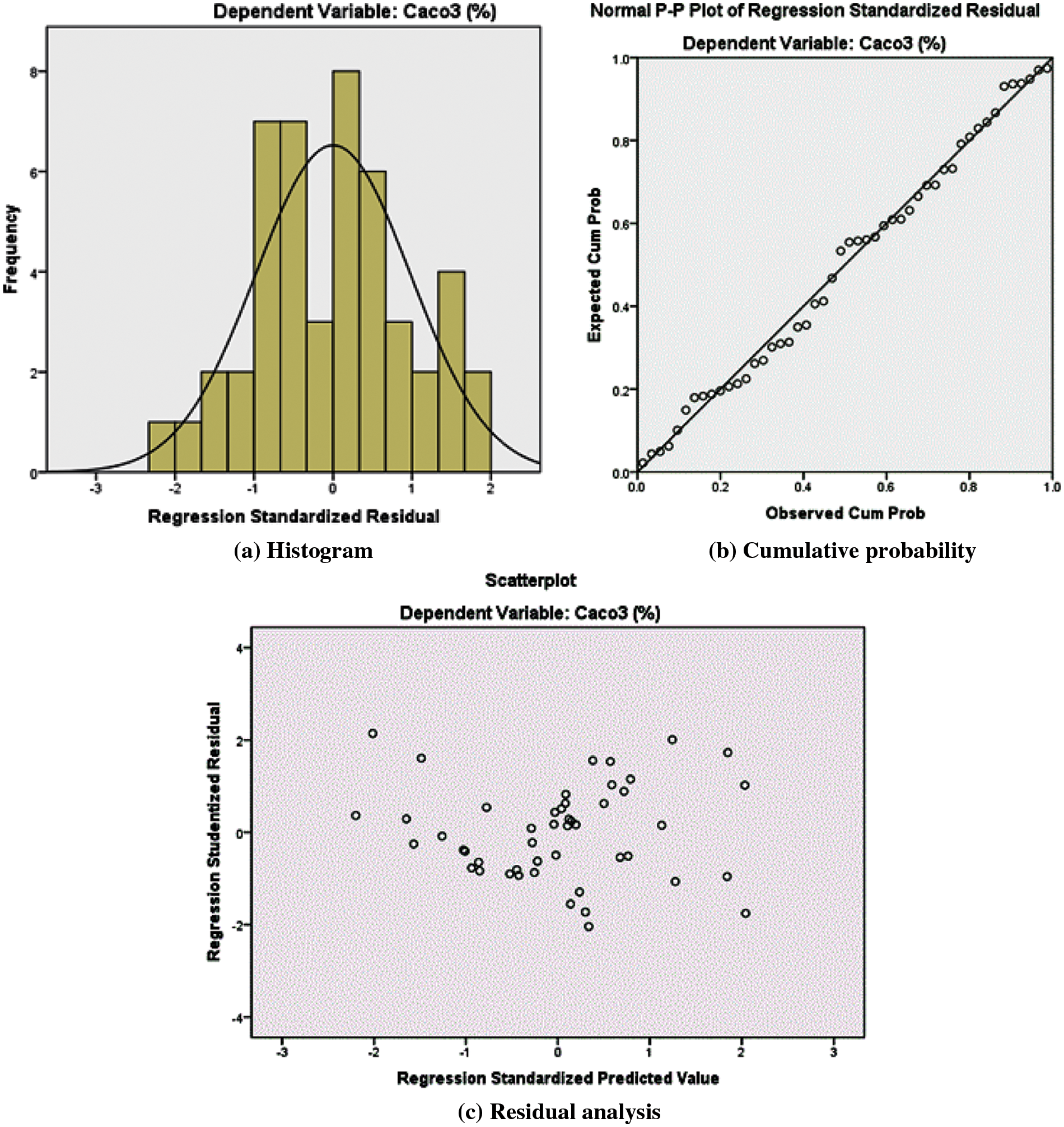
Figure 6: Histogram, cumulative probability, and residual analysis for the for the prediction models of soil CaCO3

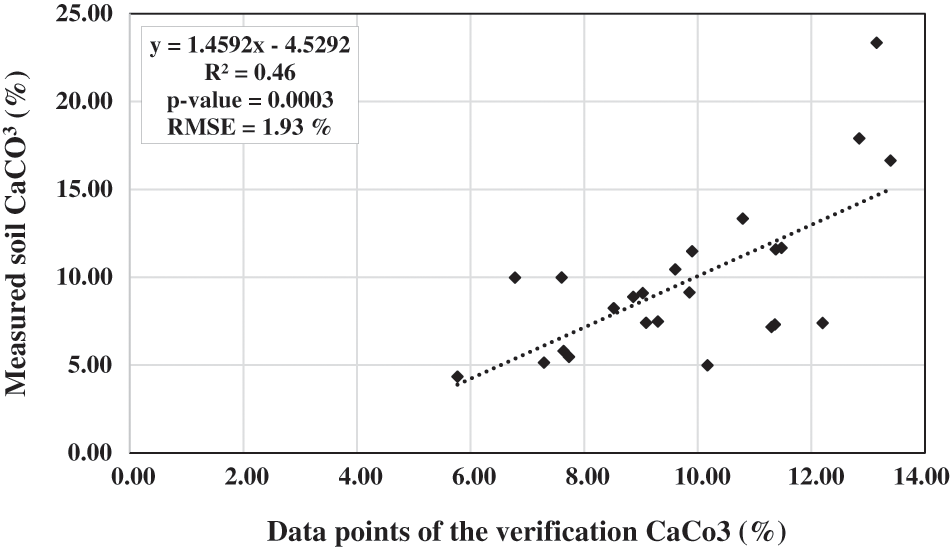
Figure 7: The validation CaCO3 data points vs. corresponding measured values

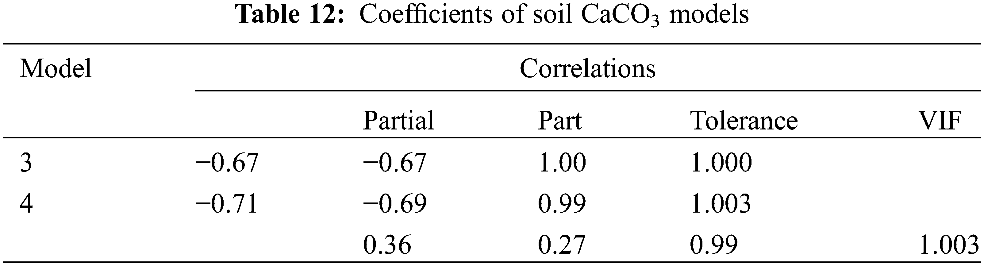
Based on the coefficients analysis including a Tolerance (T) value of 1.000 and a Variance Inflation Factor (VIF) of 1.00 (Table 12). However, Model-3 showed the most valid correlation between the measured and predicted soil CaCO3.

The Fig. 8 represents the strong positive correlation among the studied model using the different parameters to figure out the CaCO3 prediction from other characteristics linked with these parameters using the BSI and NDSI indices taken by Sentinel-2 satellite imagery.

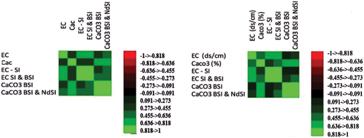
Figure 8: Correlation matrix among the satellite image crop Model-1 and Model-2. The red color represents the strong negative correlation to light green (strong positive correlation)

As shown in Figs. 9 and 10, predicted soil data points were interpolated and mapped by using geostatistical procedures (i.e., kriging) available in ArcGIS software program (Ver. 10.7.1). predicted maps of soil EC from Model-1 & Model-2 and soil CaCO3 from Model-3 & Model-4 were generated to clarify the spatial distribution of predicted values.

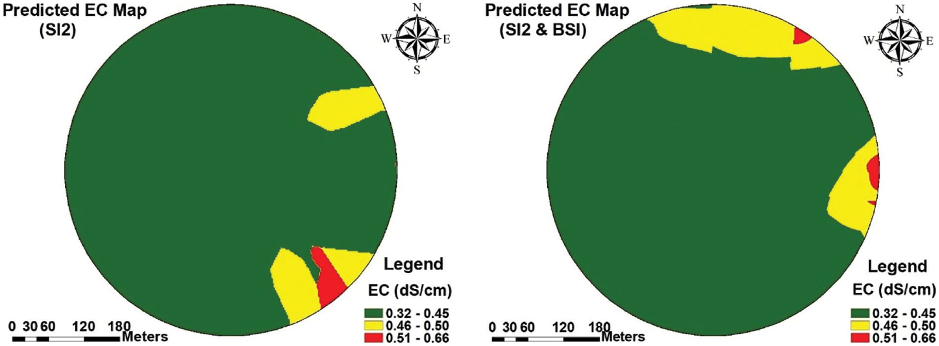
Figure 9: Predicted soil EC map from Model-1 (SI2) and Model-2 (SI2 & BSI)

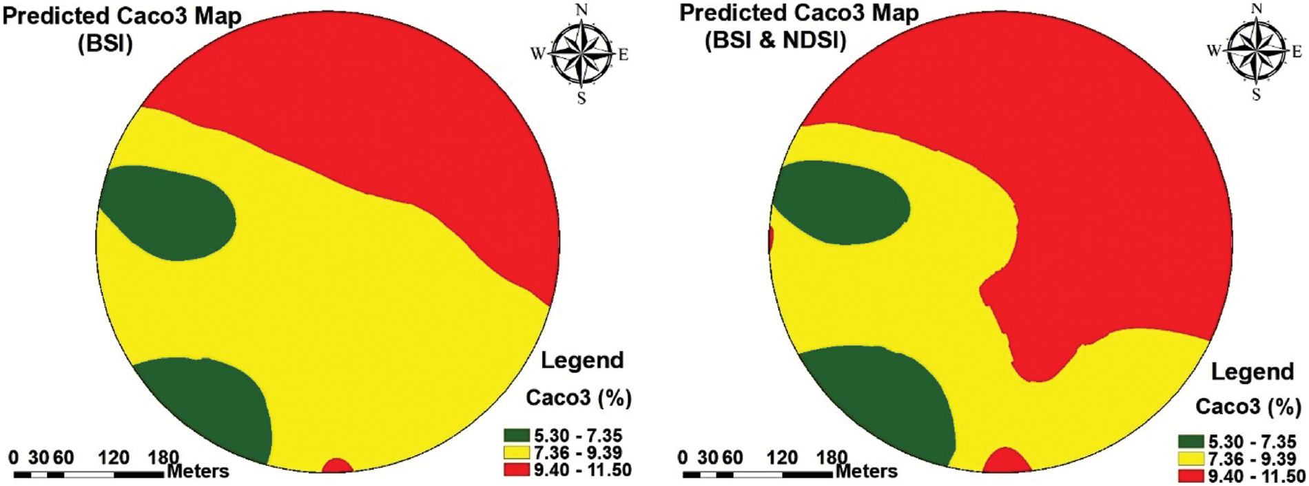
Figure 10: Predicted soil CaCO3 map from Model-3 (BSI) and Model-4 (BSI & NDSI)

4  Discussion

Particularly in arid and semi-arid locations, soil salinity is a major contributor to desertification, land degradation, and other environmental hazards. By mapping the electrical conductivity (EC) of the soil, it is possible to determine the severity and scope of the salt spread in the afflicted areas, which is the first step in coming up with a remedy. A possible way to map salinity is by combining the capability of high-resolution satellite images with remote sensing methods, as this enables large-scale monitoring and offers great accuracy and efficiency. The similar results were reported using S2A satellite and landset-8 data to evaluate the salt characteristics and relate with the EC of the data with different regression analysis. The study concludes that the suggested strategy for modeling salinity and mapping soil EC can be regarded as an efficient tool for soil salinity monitoring [34]. Similar regression analysis techniques were also suggested by other researchers to evaluate the soil salinity characteristics and compare it with EC for stimulating soil salinity. The study area and the used regression algorithms affect how well these methods perform [35,36].

To correlate satellite-derived salinity indices with 28 field samples and produce salinity maps for years of research, Gorji et al. [37] used linear and exponential regression analysis techniques for data validation study. Similarly, partially least squares regression (PLSR), technique developed by Qu et al. [38], has been proven to be effective in retrieving soil salinity from hyperspectral data. The outcomes showed that the calibrated PLSR model could be utilized as a method to accurately recover soil salinity. The current study also used the S2A spectral indices and correlate the indices using different regression analysis techniques. The study results suggested that ANOVA results (Table 5) confirmed the significant relationship between the soil indices and soil EC for the two models. The accuracy of the models was performed, as shown in Table 6 and Fig. 2. The validation R2 value of Model-1 (SI2) was 0.48, which was slightly higher than the validation R2 value (0.47) of Model-2 (SI2 & BSI) and confirmed by the RMSE value of 1.32% for Model-1, which was lower than the RMSE value of 6.42% for Model-2. The results of Model-1 (SI2) agree with that of [39], which confirmed the capability of salinity index-2 in predicting the soil EC. The regression strength of the two prediction models of soil EC was performed through the histogram analysis, the normal probability plot and the residual analysis as shown in Fig. 3.

However, better management scales are also an important subject to address. In this regard, remote sensing technologies can make significant contributions to agriculture monitoring [40] and advance our knowledge of the effects of environmental changes [41] within the context of precision agriculture. With the launches of Sentinel-2 A + B, many of the restrictions in the use of remote sensing techniques for precision agriculture in earlier years [42] have been removed. The Sentinel-2 constellation was created primarily to address the demands of the agricultural community, including farmers and academic researchers with a focus on global agricultural development. It has better spatial, spectral, and temporal resolution. Based on the facts and farmers friendly characteristics, the current study used Sentinel-2 system for the prediction of different biotic and abiotic stresses evaluation at early stage would be foremost to overcome the soil related issues for crop productivity [43].

Since there are currently numerous models or indicators that represent these functions, many scientific works have focused on understanding and simulating the physical, chemical, and biological processes that underlie these various functions [44]. These models and indicators require the use of exact geographically referenced soil information as inputs in order to be fully operational in aiding decisions made at local, national, and global levels [45]. Similar results reported by Vandour et al. [45] evaluate the soil ecosystem functions using spatial levels model using S2A multispectral satellite images. The results partial least squares regression models based on 72 and 143 S2A spectra, respectively. They also evaluate the pH, sand, silt clay, calcium carbonate, iron, and soil organic carbon. Furthermore, the predictive RMSE analysis, cross coefficient and ratio of performance to deviation was also conducted. The results suggested that performance outcomes were recorded more than or equal to 1.40 and 0.50 was recorded, respectively, however, near intermediate performance outcomes were recorded 1.30, 1.40, 0.39 and 0.50, respectively.

The study’s findings demonstrate what can be anticipated in terms of Sentinel-2 pictures’ regional-scale forecasting abilities. The current study demonstrates the two models with a significant correlation between the measured and predicted soil CaCO3 by soil indices (R2 values ranging between 0.45 and 0.53, respectively) using the S2A spectra. Another study recorded the contrasting results suggested that the RMSECV and cross validation using (R2cv) from the residual prediction deviation reported that values between 1.40 and 1.80 indicate models with a moderate level of predictive capability; values between 1 and 1.40 indicate models with a bad level of predictive capability; and values below 1 indicate very subpar models that should not be employed [46,47]. Similarly, the Model-3 showed the most valid correlation between the measured and predicted soil CaCO3. The results of Model-3 (BSI) were similar to the findings of [20], which estimated soil CaCO3 from two bare soil composites of 30 m resolution Landsat image with R2 value of 0.44.

5  Conclusion

The current study was based on the modeling of the relationship between the soil indices calculated from Sentinel-2 satellite image and the concentrations of laboratory-estimated soil properties. The linear regression models were applied to the soil indices on the on the topsoil of agricultural fields in Sudan for the prediction soil EC and CaCO3. The specific conclusions of this study could be summarized as follows: The linear regression results of soil EC showed two models with the most significant correlation between the soil EC estimated in laboratory and the soil indices: SI2 (Model-1) and the BSI (Model-2). The validation confirmed the validity of Model-1 with high R2 (0.48) and less RMSE value of 1.32%. Also, the linear regression results of soil CaCO3 showed two models with the most significant correlation between the soil CaCO3 estimated in laboratory and the soil indices: BSI (Model-3) and BSI & NDSI (Model-4). The validation confirmed the validity of Model-3 with high R2 (0.48) and less RMSE value of 1.29%.

Acknowledgement: The authors are grateful to the Deanship of Scientific Research, King Saud University for funding this study through the Vice Deanship of Scientific Research Chairs. The unlimited cooperation and support extended by Al Rajhi International for Investment (RAII) in carrying out the research work are gratefully acknowledged.

Funding Statement: The authors received no specific funding for this study.

Author Contributions: All listed authors should have substantially contributed to the manuscript and have approved the final submitted version, which should include a description of each author’s specific work and contributor ship. Conceptualization, A.M.Z. and K.A.A.; Data curation, A.M.Z. and E.T.; Formal analysis, A.M.Z. and R.M.; Investigation, K.A.A. and E.T.; Methodology, A.M.Z. and A.A.A.; Resources, A.M.Z.; Supervision, K.A.A. and E.T.; Writing—original draft, A.M.Z.; Writing—review & editing, A.M.Z. and A.A.A. and R.M. All authors have read and agreed to the published version of the manuscript.

Conflicts of Interest: The authors declare that they have no conflicts of interest to report regarding the present study.

References

1. El Harti, A., Lhissou, R., Chokmani, K., Ouzemou, J., Hassouna, M. et al. (2016). Spatiotemporal monitoring of soil salinization in irrigated Tadla Plain (Morocco) using satellite spectral indices. International Journal of Applied Earth Observation and Geoinformation, 50(4), 64–73. https://doi.org/10.1016/j.jag.2016.03.008 [Google Scholar] [CrossRef]

2. Valipour, M. (2014). Drainage, waterlogging, and salinity. Archives of Agronomy and Soil Science, 60(12), 1625–1640. https://doi.org/10.1080/03650340.2014.905676 [Google Scholar] [CrossRef]

3. Ramos, T. B., Castanheira, N., Oliveira, A. O., Paz, A. M., Darouich, H. et al. (2020). Soil salinity assessment using vegetation indices derived from Sentinel-2 multispectral data application to Lezíria Grande, Portugal. Agricultural Water Management, 241. [Google Scholar]

4. Minhas, P. S., Ramos, T. B., Ben-Gal, A., Pereira, L. S. (2020). Coping with salinity in irrigated agriculture: Crop evapotranspiration and water management issues. Agricultural Water Management, 227(8), 105832. https://doi.org/10.1016/j.agwat.2019.105832 [Google Scholar] [CrossRef]

5. Panagos, P., Borrelli, P., Robinson, D. (2020). FAO calls for actions to reduce global soil erosion. Mitigation and Adaptation Strategies for Global Change, 25(5), 789–790. https://doi.org/10.1007/s11027-019-09892-3 [Google Scholar] [CrossRef]

6. Zaman, M., Shahid, S. A., Heng, L. (2018). Guideline for salinity assessment, mitigation and adaptation using nuclear and related techniques. Springer Nature. [Google Scholar]

7. Corwin, D. L. (2021). Climate change impacts on soil salinity in agricultural areas. European Journal of Soil Science, 72(2), 842–862. https://doi.org/10.1111/ejss.13010 [Google Scholar] [CrossRef]

8. Haneda, Y., Okada, M., Suganuma, Y., Kitamura, T. (2020). A full sequence of the Matuyama–Brunhes geomagnetic reversal in the Chiba composite section, Central Japan. Progress in Earth and Planetary Science, 7(1), 1–22. https://doi.org/10.1186/s40645-020-00377-5 [Google Scholar] [CrossRef]

9. Chen, Y., Qiu, Y., Zhang, Z., Zhang, J., Chen, C. et al. (2020). Estimating salt content of vegetated soilat different depths with Sentinel-2 data. PeerJ, 8, e10585. https://doi.org/10.7717/peerj.10585 [Google Scholar] [PubMed] [CrossRef]

10. Allbed, A., Kumar, L. (2013). Soil salinity mapping and monitoring in arid and semi-arid regions using remote sensing technology: A review. Advances Remote Sensing, 2(4), 373–385. https://doi.org/10.4236/ars.2013.24040 [Google Scholar] [CrossRef]

11. Umer, M. I., Rajab, S. M., Ismail, H. K. (2020). Effect of CaCO3 form on soil inherent quality properties of calcareous soils. Materials Science Forum, 1002, 459–467. https://doi.org/10.4028/www.scientific.net/MSF.1002.459 [Google Scholar] [CrossRef]

12. Ibrahim, S. I. (2008). Soils of the arid and semi-arid regions. In: Verheye, W.H. (Ed.Land use, land cover and soil sciences. Oxford, UK: UNESCO-EOLSS Publishers. [Google Scholar]

13. Shit, P. K., Bhunia, G. S., Maiti, R. (2016). Spatial analysis of soil properties using GIS based geostatistics models. Modeling Earth Systems and Environment, 2(2), 1–6. https://doi.org/10.1007/s40808-016-0160-4 [Google Scholar] [CrossRef]

14. Gomez, C., Lagacherie, P., Coulouma, G. (2012). Regional predictions of eight common soil properties and their spatial structures from hyperspectral Vis-NIR data. Geoderma, 189(1), 176–185. https://doi.org/10.1016/j.geoderma.2012.05.023 [Google Scholar] [CrossRef]

15. Vaudour, E., Gilliota, J. M., Bel, L., Lefevre, J., Chehdi, K. (2016). Regional prediction of soil organic carbon content over temperate croplands using visible near-infrared airborne hyperspectral imagery and synchronous field spectra. International Journal of Applied Earth Observation and Geoinformation, 49(6), 24–38. https://doi.org/10.1016/j.jag.2016.01.005 [Google Scholar] [CrossRef]

16. Diek, S., Fornallaz, F., Schaepman, M. E., Jong, R. D. (2017). Barest pixel composite for agricultural areas using landsat time series. Remote Sensing, 9(12), 1245. https://doi.org/10.3390/rs9121245 [Google Scholar] [CrossRef]

17. Martinez, J. (2017). Relationship between crop nutritional status, spectral measurements and Sentinel 2 images. Agronomia Colombiana, 35(2), 205–215. https://doi.org/10.15446/agron.colomb.v35n2.62875 [Google Scholar] [CrossRef]

18. Lobell, D. B., Lesch, S. M., Corwin, D. L., Ulmer, M. G., Anderson, K. A. et al. (2010). Regional-scale assessment of soil salinity in the Red River Valley using multi-year MODIS EVI and NDVI. Journal of Environmental Quality, 39(1), 35–41. https://doi.org/10.2134/jeq2009.0140 [Google Scholar] [PubMed] [CrossRef]

19. Guo, B., Han, B., Yang, F., Fan, Y., Jiang, L. et al. (2019). Salinization information extraction model based on VI–SI feature space combinations in the Yellow River Delta based on Landsat 8 OLI image. Geomatics, Natural Hazards and Risk, 10(1), 1863–1878. https://doi.org/10.1080/19475705.2019.1650125 [Google Scholar] [CrossRef]

20. Safanelli, J. L., Chabrillat, S., Ben-Dor, E., Dematte, J. (2020). Multispectral models from bare soil composites for mapping topsoil properties over Europe. Remote Sensing, 12(9), 1369. https://doi.org/10.3390/rs12091369 [Google Scholar] [CrossRef]

21. Golia, E. E., Diakoloukas, V. (2022). Soil parameters affecting the levels of potentially harmful metals in Thessaly area, Greece: A robust quadratic regression approach of soil pollution prediction. Environmental Science and Pollution Research, 29(20), 29544–29561. https://doi.org/10.1007/s11356-021-14673-0 [Google Scholar] [PubMed] [CrossRef]

22. Davis, E., Wang, C., Dow, K. (2019). Comparing Sentinel-2 MSI and Landsat 8 OLI in soil salinity detection: A case study of agricultural lands in coastal North Carolina. International Journal of Remote Sensing, 40(16), 6134–6153. https://doi.org/10.1080/01431161.2019.1587205 [Google Scholar] [CrossRef]

23. Estefan, G., Sommer, R., Ryan, J. (2013). Methods of soil, plant, and water analysis. A Manual for the West Asia and North Africa Region, 3, 65–119. [Google Scholar]

24. Loiseau, A., Asila, V., Boitel-Aullen, G., Lam, M., Salmain, M. et al. (2019). Silver-based plasmonic nanoparticles for and their use in biosensing. Biosensors, 9(2), 78. https://doi.org/10.3390/bios9020078 [Google Scholar] [PubMed] [CrossRef]

25. Bannari, A., El-Battay, A., Hameid, N., Tashtoush, F. (2017). Salt-affected soil mapping in an arid environment using semi-empirical model and Landsat-OLI data. Advances in Remote Sensing, 6(4), 260–291. https://doi.org/10.4236/ars.2017.64019 [Google Scholar] [CrossRef]

26. Allbed, A., Kumar, L., Aldakheel, Y. Y. (2014). Assessing soil salinity using soil salinity and vegetation indices derived from IKONOS high-spatial resolution imageries: Applications in a date palm dominated region. Geoderma, 230(8), 1–8. https://doi.org/10.1016/j.geoderma.2014.03.025 [Google Scholar] [CrossRef]

27. Jamalabad, M. S., Akbar, A. A. (2004). Forest canopy density monitoring, using satellite images. Proceedings of the 20th ISPRS Congress, Commission VII, pp. 244–249. Istanbul. [Google Scholar]

28. Douaouia, A., Nicolasb, H., Walter, C. (2006). Detecting salinity hazards within a semiarid context by means ofcombining soil and remote-sensing data. Geoderma, 134(1), 217–230. https://doi.org/10.1016/j.geoderma.2005.10.009 [Google Scholar] [CrossRef]

29. Abbas, A., Khan, S. (2007). Using remote sensing techniques for appraisal of irrigated soil salinity. International Congress on Modelling and Simulation (MODSIM 2007), pp. 2632–2638. New Zealand, Bright. [Google Scholar]

30. Khan, S. H., Bhatti, B. M. (2001). Effect of autoclaving, toasting, and cooking onchemical composition of hatchery waste meal. Pakistan Veterinary Journal, 21(1), 22–26. [Google Scholar]

31. Gitelson, A. A., Kaufman, Y. G., Merzlyak, M. N. (1996). Use of a green channel in remote sensing of global vegetation from EOS-MODIS. Remote Sensing of Environment, 58(3), 289–298. https://doi.org/10.1016/S0034-4257(96)00072-7 [Google Scholar] [CrossRef]

32. Qi, J., Chehbouni, A., Huete, A. R., Kerr, Y. H., Sorooshian, S. (1994). A modified soil adjusted vegetation index. Remote Sensing of Environment, 48(2), 119–126. https://doi.org/10.1016/0034-4257(94)90134-1 [Google Scholar] [CrossRef]

33. Jaber, S. M., Lant, C. L., Al-Qinna, M. I. (2011). Estimating spatial variations in soil organic carbon using satellite hyperspectral data and map algebra. International Journal of Remote Sensing, 32(18), 5077–5103. https://doi.org/10.1080/01431161.2010.494637 [Google Scholar] [CrossRef]

34. Taghadosi, M. M., Hasanlou, M., Eftekhari, K. (2019). Retrieval of soil salinity from Sentinel-2 multispectral imagery. European Journal of Remote Sensing, 52(1), 138–154. https://doi.org/10.1080/22797254.2019.1571870 [Google Scholar] [CrossRef]

35. Vermeulen, D., Niekerk, A. V. (2017). Machine learning performance for predicting soil salinity using different combinations of geomorphometric covariates. Geoderma, 299, 1–12. https://doi.org/10.1016/j.geoderma.2017.03.013 [Google Scholar] [CrossRef]

36. Shahabi, M., Jafarzadeh, A. A., Neyshabouri, M. R., Ghorbani, M. A., Kamran, K. V. (2017). Spatial modeling of soil salinity using multiple linear regression, ordinary kriging and artificial neural network methods. Archives of Agronomy and Soil Science, 63(2), 151–160. https://doi.org/10.1080/03650340.2016.1193162 [Google Scholar] [CrossRef]

37. Gorji, T., Sertel, E., Tanik, A. (2017). Monitoring soil salinity via remote sensing technology under data scarce conditions: A case study from Turkey. Ecological Indicators, 74, 384–391. https://doi.org/10.1016/j.ecolind.2016.11.043 [Google Scholar] [CrossRef]

38. Qu, Y., Jiao, S., Lin, X. (2008). A partial least square regression method to quantitatively retrieve soil salinity using hyper-spectral reflectance data. Proceedings of SPIE—The International Society for Optical Engineering, vol. 7147, pp. 484–492. Bellingham, Washington USA. [Google Scholar]

39. Solangi, K. A., Siyal, A. A., Wu, Y., Abbasi, B., Solangi, F. et al. (2019). An assessment of the spatial and temporal distribution of soil salinity in combination with field and satellite data: A case study in Sujawal district. Agronomy, 9(12), 8694. https://doi.org/10.3390/agronomy9120869 [Google Scholar] [CrossRef]

40. Mulla, D. J. (2013). Twenty five years of remote sensing in precision agriculture: Key advances and remaining knowledge gaps. Biosystems Engineering, 114(4), 358–371. https://doi.org/10.1016/j.biosystemseng.2012.08.009 [Google Scholar] [CrossRef]

41. Yang, J., Gong, P., Fu, R., Zhang, M., Chen, J. et al. (2013). The role of satellite remote sensing in climate change studies. Nature Climate Change, 3(10), 875–883. https://doi.org/10.1038/nclimate1908 [Google Scholar] [CrossRef]

42. Zhang, N., Wang, M., Wang, N. (2002). Precision agriculture—A worldwide overview. Computers and Electronics in Agriculture, 36(2–3), 113–132. https://doi.org/10.1016/S0168-1699(02)00096-0 [Google Scholar] [CrossRef]

43. Segarra, J., Buchaillot, M. L., Araus, J. L., Kefauver, S. C. (2020). Remote sensing for precision agriculture: Sentinel-2 improved features and applications. Agronomy, 10(5), 641. https://doi.org/10.3390/agronomy10050641 [Google Scholar] [CrossRef]

44. Baveye, P. C., Baveye, J., Gowdy, J. (2016). Soil ecosystem services and natural capital: Critical appraisal of research on uncertain ground. Frontiers in Environmental Science, 4(10), 41. https://doi.org/10.3389/fenvs.2016.00041 [Google Scholar] [CrossRef]

45. Vaudoura, E., Gomez, C., Fouad, Y., Lagacherie, P. (2019). Sentinel-2 image capacities to predict common topsoil properties of temperate and Mediterranean agroecosystems. Remote Sensing of Environment, 223(1), 21–33. https://doi.org/10.1016/j.rse.2019.01.006 [Google Scholar] [CrossRef]

46. Chang, C., Laird, D., Mausbach, M. J., Hurburgh, C. R. (2001). Near-infrared reflectance spectroscopy-principal components regression analyses of soil properties. Soil Science Society of America Journal, 65(2), 480–490. https://doi.org/10.2136/sssaj2001.652480x [Google Scholar] [CrossRef]

47. Rossel, R. V., Walvoort, D. J., McBratney, A. B., Janik, L. J., Skjemstad, J. O. (2006). Visible, near infrared, mid infrared or combined diffuse reflectance spectroscopy for simultaneous assessment of various soil properties. Geoderma, 131(1–2), 59–75. https://doi.org/10.1016/j.geoderma.2005.03.007 [Google Scholar] [CrossRef]

48. Navarro, J. A., Abarquero, N. A., Fernandez, A., Esteban, J., Rodriguez, P. et al. (2019). Integration of UAV, Sentinel-1, and Sentinel-2 data for mangrove plantation aboveground biomass monitoring in Senegal. Remote Sensing, 11(1), 77. [Google Scholar]

Appendix

Abbreviations

Sentinel-2 imagery data bands (Navarro et al. [48])