Phyton-International Journal of Experimental Botany

DOI: 10.32604/phyton.2022.021096

ARTICLE

Research on WNN Greenhouse Temperature Prediction Method Based on GA

Wenbin Dai1, Lina Wang1,2,*, Binrui Wang1, Xiaohong Cui1 and Xue Li1

1College of Mechanical and Electronic Engineering, China Jiliang University, Hangzhou, 310018, China
2Key Laboratory of Intelligent Manufacturing Quality Big Data Tracing and Analysis of Zhejiang Province, China Jiliang University, Hangzhou, 310018, China
*Corresponding Author: Lina Wang. Email: 19A0102172@cjlu.edu.cn
Received: 27 December 2021; Accepted: 03 February 2022

1  Introduction

The semi-independent and semi-closed greenhouse environment is a unique advantage of greenhouse agricultural production. Compared with the traditional agricultural production in a fully open environment, the greenhouse provides a more stable environment for crops and reduces the influence of the external environment. This production process has good environmental adaptability and efficient economic output. In agricultural production, temperature control is the primary problem, which directly affects not only crop growth but also the economic output of agriculture [1–4]. Therefore, some researchers have studied the greenhouse from the perspective of the greenhouse model. Traditional modeling generally builds differential equation models of the greenhouse based on the physical relationship of the greenhouse environment and is named mechanism modeling. Singh et al. developed microclimate mechanism models to predict air temperatures in plant communities and leaves by describing energy and mass transfer processes [5]. Costantino et al. [6] proposed a new modeling method to simulate the operation and energy performance of the dynamic greenhouse system for the climate control energy consumption of mechanically ventilated greenhouses. Gerasimov et al. [7] proposed an adaptive scheme of greenhouse system by mechanism modeling to solve the multiple input and multiple output (MIMO) problems of greenhouse temperature, humidity and carbon dioxide concentration. Liu et al. [8] proposed a wall temperature estimation method based on the energy balance for the environment model and used a mechanistic method to estimate the temperature and humidity in a Chinese solar greenhouse. The mechanism model results based on the specific environment are more accurate and detailed. But on the other hand, the modeling process is complicated and difficult, and the versatility is poor, which also makes this method unable to be used in all scenarios [9].

The emergence of intelligent algorithms has led to new approaches. Artificial Neural Network (ANN), a kind of mathematical model structure to simulate the biological mechanism of the human brain, has particular learning ability and adaptability [10–12]. Manonmani et al. [13] adopted a neural predictive controller and nonlinear autoregressive moving average controller (NARMA-L2) to simulate prediction and control of greenhouse temperature and humidity. Gandhi et al. [14] applied Levenberg Marquardt back-propagation algorithm to train and optimize the neural network, which combined with a neural predictive control (NPC) to achieve greenhouse temperature control and tracking. Jung et al. [15] compared nonlinear autoregressive exogenous model (NARX), recurrent neural network long- and short-term memory (RNN-LSTM) to predict the changes of environmental factors in the greenhouse to find the best greenhouse control strategy. Hongkang et al. [16] compared the dynamic backpropagation algorithm model based on recursive neural network (RNN) and predicted the temperature and humidity of the greenhouse. Compared with mechanism modeling, neural network modeling has the data-driven characteristics, and a wider range of applications and good model performance [10,17,18]. Therefore, good performance and easy realization of the model in the greenhouse make it widely used.

Wavelet neural network is a kind of network which consists of wavelet basis function and forward feedback network structure. Compared with other network models, wavelet neural network (WNN) has better accuracy and stability and faster training speed in short-term prediction and is widely used in other fields [19,20]. Feng et al. [21] and Falamarzi et al. [22] both studied the problem of WNN and other neural networks to predict regional climate and evapotranspiration changes, and achieved good predictive effects. Nayak et al. [23] used WNN to predict hydrological characteristics such as the flow duration curve in the area. Sharma et al. [24] proposed a time series prediction hybrid WNN for short-term solar irradiance prediction and applied it in tropical areas. These researches show that the wavelet neural network has a good fitting ability, faster learning speed and better prediction effect for the short-term prediction models. In the greenhouse modeling process, the accuracy and train speed of the model and prediction are also important goals. However, few researchers studied on the WNN and the applications are ignored in greenhouses. Therefore, this paper aims to investigate the WNN model predicting the trend of the temperature in the greenhouse. Matlab is a mathematical platform that brings together programming and numerical computation, analysis, algorithm development and modelling. The greenhouse modelling and simulation processes were carried out in Matlab R2016a

During the training process of data model, the initial random weight leads to uncertainty of training direction and reduces the training efficiency. Some researchers took the models with global optimization algorithms and obtained better positive effects. Jin et al. [25] proposed an improved genetic algorithm with engineering constraint rules (R-GA) to effectively and practically solve the dynamic economic optimal control problem in greenhouse environments. Yadav et al. [26] introduced a PSO-GA based hybrid training algorithm with Adam Optimization. Through the multi-algorithm fusion method, the local optimal problem of a single algorithm is compensated, and the global search ability and the accuracy of medical diagnosis are significantly improved. Taghavi et al. [27] applied GA to optimize the neural network model for the air-fuel mixture properties, which has greatly shortened the time needed to train the networks. Panahi et al. [28] proposed an integrated ANN model with the antlion optimization (ANN-ALO) for predicting freshwater production in a seawater greenhouse. Comparing model performance in tests, the prediction error of ANN-ALO model outperforms the ANN, ANN-particle swarm optimization, ANN-bat algorithms. Tian et al. [29] proposed an improved enhanced long-term memory neural network prediction model combined with the sparrow search algorithm, which has the best prediction performance and prediction accuracy compared with other short-term models. The genetic algorithm (GA) is a typical global optimization algorithm. ANN with the genetic algorithm (GA-ANN) can fully search for target individuals in a large range, and avoid the local optimal situation through multi-generation inheritance, mutation, and exchange operations in the evolutionary process. GA can overcome the shortcomings of a single ANN that is insensitive to weights and thresholds, and improve the accuracy and training speed of prediction models. In the following paper, the GA is used to optimize the WNN model, which is compared and verified with the BPNN and the single WNN.

This paper is organized as follows: the network principles and characteristics of WNN and GA-WNN are presented in the second paragraph. The simulation results and analysis of the model are presented in the third paragraph. The last paragraph is the summary and conclusion of the whole paper.

2  Methodology

2.1 Preliminary Analysis of Greenhouse Model

Fig. 1 is the schematic diagram of a greenhouse system, which consists of the greenhouse part and the control part [2]. The greenhouse part is composed of the external environment, the internal environment and crops. It constitutes a complete greenhouse environment and provides a growth environment for crops. The control part mainly includes sensors, greenhouse models, and controllers and control equipment. It consists of the detection, modeling, control and feedback part of greenhouse system, which plays a crucial role in greenhouse regulation. The most critical part in the greenhouse system is the greenhouse model and the greenhouse controller. The greenhouse model reflects the relationship between environmental factors in the greenhouse and affects the target control of the controller [30,31]. So the greenhouse modeling is vital for the greenhouse system.

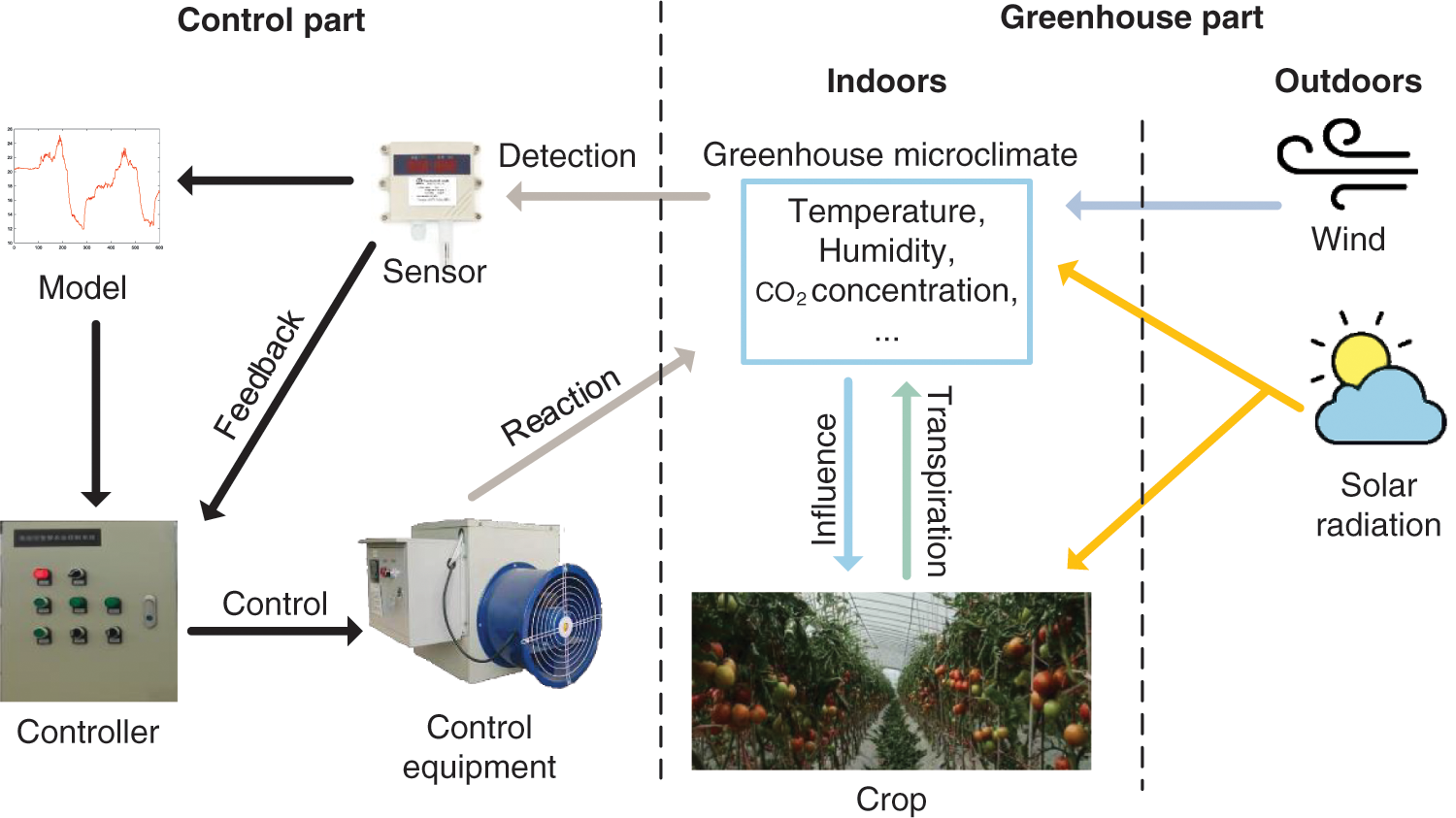
Figure 1: Common greenhouse structure

The parameters in the greenhouse models can be divided into external environmental factors, internal environmental factors, control equipment factors and influencing crops factors. The external factors include: external temperature, external humidity, external wind speed, external light intensity. These factors are directly affected by external weather and climate, and have greater uncertainty. They are generally used as input of the greenhouse model. Internal factors generally include: internal temperature, internal humidity, internal CO2 concentration and so on. Internal factors relate to the growth and development of crops, which are the direct goals of the greenhouse control. The factors of the greenhouse equipment result from the artificial equipment, such as the illumination intensity generated by the auxiliary light, the humidifier humidification rate, the output power of the heating device, the size of the opening of the vent and the production rate of the CO2 supplementary device. These factors directly affect the internal crops and are the parameters of the greenhouse environment control. The influencing crops factors are mainly the result from photosynthesis and respiration during crop growth, and directly feed back to the internal environment of the greenhouse. But it is difficult to detect and control them.

The influences of system nonlinearity and coupling between factors is practical. It is hard to analyze greenhouse temperature by the mechanism method. However, relying on physical relationships to establish the models is unnecessary by intelligent algorithms such as neural network It avoids the problem by fitting the required data model with a large number of relevant actual data and maintains a high precision at the same time. The goal of this paper is to predict the internal greenhouse temperature after the next 15 min. The following will use neural networks for modeling and simulation prediction.

2.2 Model Parameters

In this paper, the simulation experimental data are all from the real solar greenhouse environment, and are measurement results of the actual greenhouse for tomato from January to March. Model parameters need to be more correlated with the greenhouse environment and crop growth conditions, which can also be quickly collected and tested. The parameters collected by sensors include: the external environmental parameters of the greenhouse: outdoor temperature (°C), absolute outdoor humidity (g/m3), outdoor wind speed (m/s); Internal environmental parameters of the greenhouse: indoor temperature (°C), indoor absolute humidity (g/m3), indoor CO2 concentration (ppm), Total light intensity (W/m2). These parameters have the impacts on crop growth and can be quickly collected and tested. So these parameters are used as input of the greenhouse model.

The goal of the whole model is to predict the temperature in the greenhouse, obviously for the temperature in the next 15 min (°C) as the output.

2.3 Prediction Model of Greenhouse Temperature Based on WNN

In wavelet analysis, the mother wavelet function satisfies ψ(t) ∈ L2(R). Wavelet sequence is obtained by scaling and translation.

ψa,b(t)=1|a|ψ(t−ba)a,b∈R;a≠0 (1)

where ψa,b(t) is wavelet sequence; a is the expansion factor and b is the translation factor; ψ(t) is mother wavelet function; t is time.

The continuous wavelet transform function for target signal:

Wf(a,b)≤f,Wf(a,b)=1|a|∫R⁡f(t)ψ¯⁡(t−ba)dt (2)

It is inverse transformation:

f(t)=1Cψ∫−∞∞⁡∫−∞∞1a2Wf(a,b)ψ¯⁡(t−ba)dadb (3)

And Cψ=∫R|ψ^(ω)|2|ω|dω , ψ^ is the Fourier transform of the mother wavelet function and ω is the frequency; In the above equation, f(t) is target signal; Wf(a,b) is Wavelet sequence of the target signal; f indicates the bounded signal; ψ¯(t) is the wavelet mother function.

For any signal function, its equivalent transformation can be realized by superposition of multiple wavelet sequences. This transform is similar to Fourier transform in the basic principle of transformation. But at the same time, the expansion and translation superposition of wavelet sequence is introduced to realize multi-scale refinement in time-frequency, which is more conducive to the time and frequency requirements of signal [19,32–35]. WNN is a special neural network based on the same principle of the wavelet transform. Fig. 2 is the schematic diagram of the WNN network structure, which is based on BPNN topology. The hidden layer activation functions are replaced by wavelet basis functions, while the structure of the input layer and output layer is consistent with BPNN [19,36]. The wavelet sequence of each node is obtained by translating and scaling the wavelet basis function. Multiple wavelet sequences synthesize a target output of the neural network. The following formula is the calculation of the hidden layer and output layer:

h(j)=hj(∑i=1N⁡ωijxi−bjaj) (4)

y(k)=∑j=1n⁡ωjkh(j) (5)

hj=cos⁡(1.75x)e−x22 (6)

i=1,2,3…M;j=1,2,3…L;k=1,2,3…N;

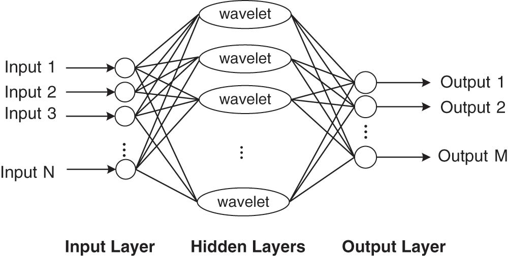
Figure 2: Structure of a wavelet neural network

The neural network contains M inputs, N outputs, and L hidden nodes; h(j) is the output of hidden layer node j; xi represents the input i of the neural network; hj(x) is the wavelet basis function of hidden layer; ωij is the weight between input node i and hidden node j; aj is the expansion variable; bj is the translation variable; y(k) is the node j output; ωjk is the weight of the connected hidden node j and the output node k.

By introducing the wavelet basis function, the output process of the network is closer to the signal decomposition, transformation, and synthesis process. The input of the hidden node realizes the multi-scale decomposition and transformation of the multi-wavelet sequence through the transformation. Then the results of multiple nodes are superimposed with each other to complete total outputs.

The common wavelet basis functions are Haar wavelet, Morlet wavelet, Mexican wavelet and Meyer wavelet. In some WNN application cases, the Morlet wavelet is the most widely used wavelet [33–34,37,38]. Morlet wavelet has no scale function and fast waveform attenuation. It is a symmetrical non-orthogonal complex wavelet, which has good applications in the decomposition and frequency analysis for complex signals. Morlet wavelet also has a good fitting ability for some complex systems in WNN [9]. Therefore, Morlet wavelet is adopted as the basis function in this paper. Eq. (7) is the output calculation process of WNN. The output weights of each wavelet basis function are connected and then superimposed to calculate the prediction output of the WNN.

hj=cos⁡(1.75x)e−x22 (7)

err=∑k=1m⁡yn(k)−y(k) (8)

{△p(t+1)=−η∂e∂p(t)p(t+1)=p(t)+△p(t+1) (9)

p stands for ωij, ωjk, aj, bj; i = 1, 2, 3…M; j = 1, 2, 3…L; k = 1, 2, 3…N;

As formulations shown above, hj is the wavelet basis function of the hidden layer; y(k) is the node k output of the output layer; yn(k) is the node k actual output of the output layer; err is the error between the output of the neural network and the actual output; p and Δp represent the weight parameters and update value of weight parameters, which can be ωij, ωjk, aj, bj. And t stands for t epoch training.

The training process of wavelet neural network adopts the gradient descent method. Calculate the gradient of each weight value p by taking partial or total differentiation of the error err. The weight value is updated step by step to approximate the optimal solution of the network. After many times of forward and reverse transmission processes, the network completes the training.

In this paper, WNN is the same as BPNN in the structure and training flow of neural network. The input layer is 7 input nodes. The output layer consists of 1 output node. Considering that the output of the hidden node is added by the weights as the output of the network, there is a linear connection between the actual output layer and the hidden layer. Therefore, the linear connection with the output layer adopts the linear transfer function Purelin. The hidden layer consists of 10 output nodes, activation function is Morlet wavelet basis function; Adam algorithm is adopted to optimize the algorithm.

2.4 Prediction Model of Greenhouse Temperature Based on GA-WNN

GA is an intelligent optimization algorithm and imitates the process of biological evolution. Based on the theory of biological evolution, the process of optimization transforms into a similar process of biological evolution through mathematical simulation operation. It searches the optimal solution from a large range of random solutions. Compared with the traditional method, the local optimal solution can be well avoided by iterating the optimal solution from a single initial value. GA also has a certain self-adaptation and self-learning abilities, and uses the change rule of probability to guide its search direction by using the individual adaptive calculation. Individuals with higher fitness have a higher survival probability, and can obtain more adaptable gene structures. Therefore, GA has faster efficiency and better results for complex combinatorial optimization problems [39–42].

Fig. 3 is the flow chart of GA-WNN. The implementation of the GA proceeds as follows:

(1) According to the network structure of WNN, the weights are initially random encoded to generate the initial population individuals.

(2) Enter the population iteration loop. Calculate the fitness functions of the current model for the target population. The higher the fitness of the individual, the better individuals can meet the need of the target

(3) The individual with the worst individual fitness is eliminated. The optimal individual is replicated to replace the missing ones.

(4) Crossover and mutation operations are performed on the population to generate a new batch of populations. The operation selection of the individual is based on the principle of the roulette wheel selection. The higher the fitness, the higher the probability of operation, so as to increase the fitness of the new batch of populations.

(5) Determines whether the loop condition terminates. If not, the new population returns to execute Steps (2), (3) and (4). If the conditions are met, the genetic algorithm is ended.

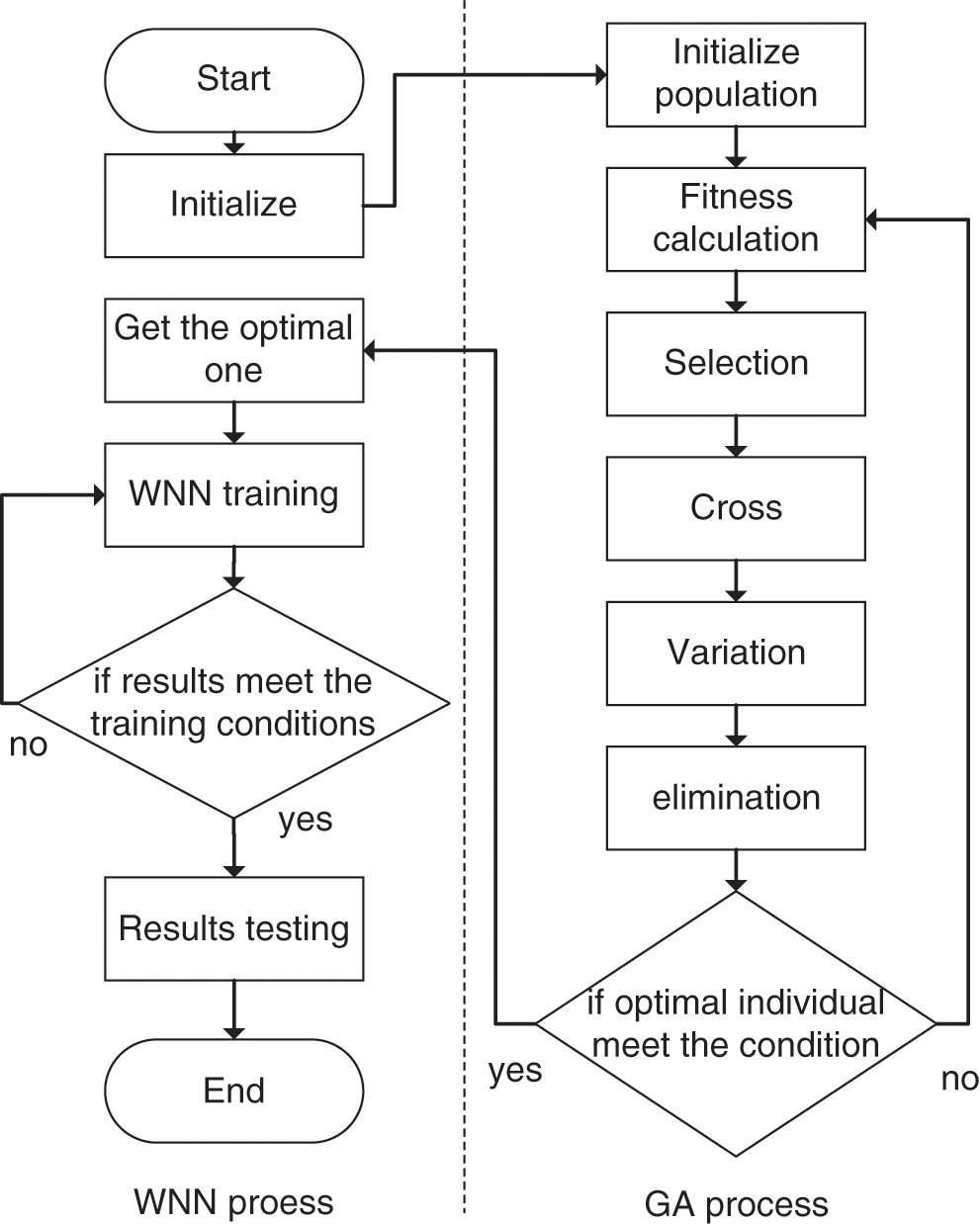
Figure 3: The flow chart of GA-WNN

Genetic algorithms are be used to filter out individuals with better weights before the WNN training. Then the individuals generated are applied to the initial weight of the WNN. The processes of the WNN are consistent with the single WNN, and the only difference is whether to optimize the initial weights. GA-WNN combines the characteristics of WNN and GA. GA provides optimal initialization weights for WNN through global iterative optimization, and avoids the uncertainty of the model training process caused by random initialization, and improving the speed of training. It is beneficial to the WNN training results under the same conditions and improves the accuracy and stability of the model, and avoids local optimal problems.

In the model, 100 initial populations are allocated in GA. The exchange probability is 0.8. The variation probability is 0.6. A total of 100 population evolution epochs are carried out in one training. It seems from Fig. 4 that the optimal fitness has remained stable since the 50th cycles. The average fitness of the 100th epoch is basically consistent with the optimal fitness and meets the needs of GA optimization. So set 100 as the maximum loop for GA. The WNN part remains the same as the structure of the single WNN network. The input layer has 7 input nodes. The output layer consists of 1 output node, where the activation function is Purelin. The hidden layer consists of 10 output nodes, the activation function is Morlet wavelet basis function; Adam algorithm is adopted to optimize the algorithm.

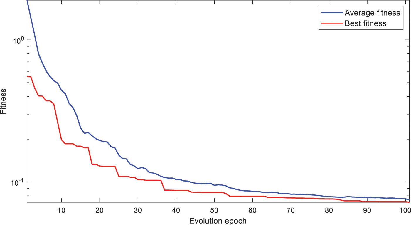
Figure 4: Fitness changes of the three network during training

3  Results and Discussion

The simulation environment is Matlab R2016a. Table 1 is the list of neural network parameters. In order to ensure the consistency of the experiment, the comparison of BPNN, WNN and GA-WNN is adopted in this paper. The networks adopt the same 7-10-1 network structure and the ADM algorithm to optimize the gradient. The collected data are from a tomato planting experiment in a solar greenhouse. This experiment recorded 72 days of data, collected at intervals of 5 min, with a total of 20552 recording points. 16432 sets of 80% data are used as training sets, and 4108 sets of the remaining 20% data are used as test sets. Under the same conditions, 500 training tests are conducted, and the results are as follows:

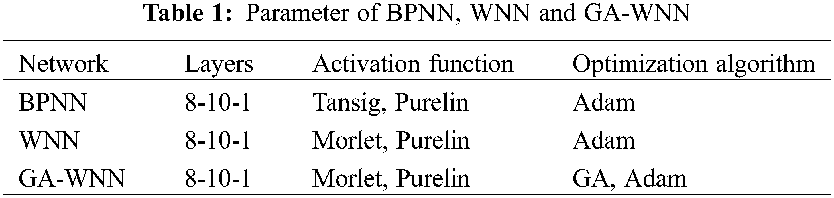
Fig. 5 shows the MSE (Mean Squared Error) distribution of the three networks after 500 independent tests. MSE is the mean of squares sum between the predicted value and the true value. It shows the dispersion and prediction result. The larger the MSE is, the higher the dispersion degree of prediction error is. The distribution of MSE results of BPNN mainly concentrated in the range of 0.364 to 0.432, and the average value was 0.4012. The MSE results of WNN ranged from 0.320 to 0.394, and the average value was 0.3590. The MSE of GA-WMM ranged from 0.312 to 0.382, and the average value was 0.3491. The results showed that WNN and GA-WNN have better prediction stability than BPNN. The prediction dispersion of WNN can be further reduced with GA to improve the prediction accuracy.

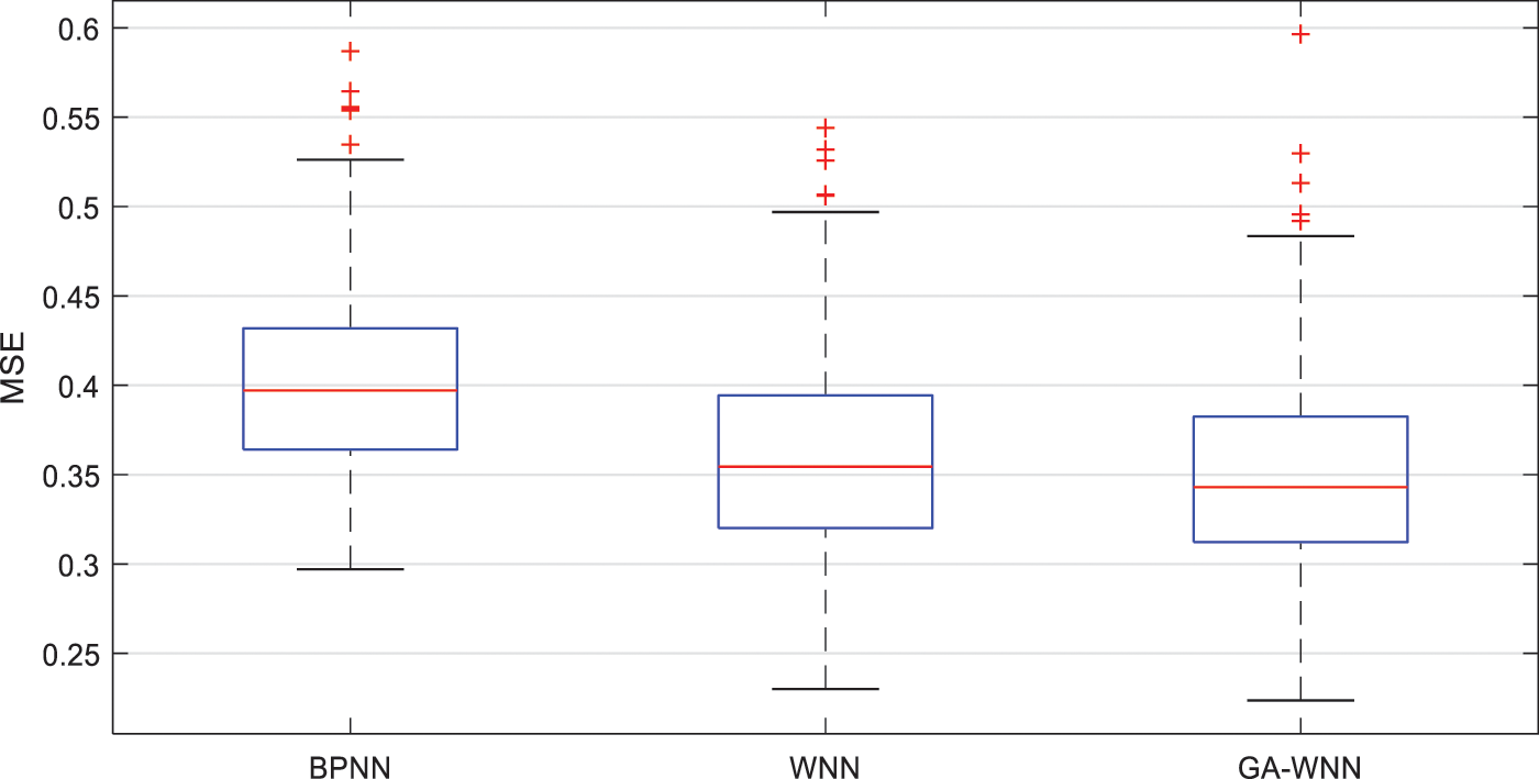
Figure 5: MSE histogram of the three network results

Fig. 6 shows MAE (Mean Absolute Squared Error) distribution of the network results after 500 independent tests. MAE is the mean of the absolute value of the difference between the actual output and the predicted output, which focuses on the error size of the whole sample. When MAE is larger, the prediction error is larger, and vice versa. The MAE of BPNN were distributed in the range of 0.349 to 0.377, and average value was 0.3654. The MAE of WNN ranged from 0.339 to 0.376, and the average value was 0.3620. MAE of GA-WMM ranged from 0.335 to 0.372, and the average value was 0.3563. The results showed that GA-WNN has a lower error than BPNN and WNN on the whole, but MAE of WNN was higher than BPNN in some samples. This may be caused by the uncertainty of the initialization and training of the WNN. MAE can be reduced by optimizing the weights of GA. With the optimization of GA, the overall MAE error of WNN is better improved, and the stability is better than that of BP.

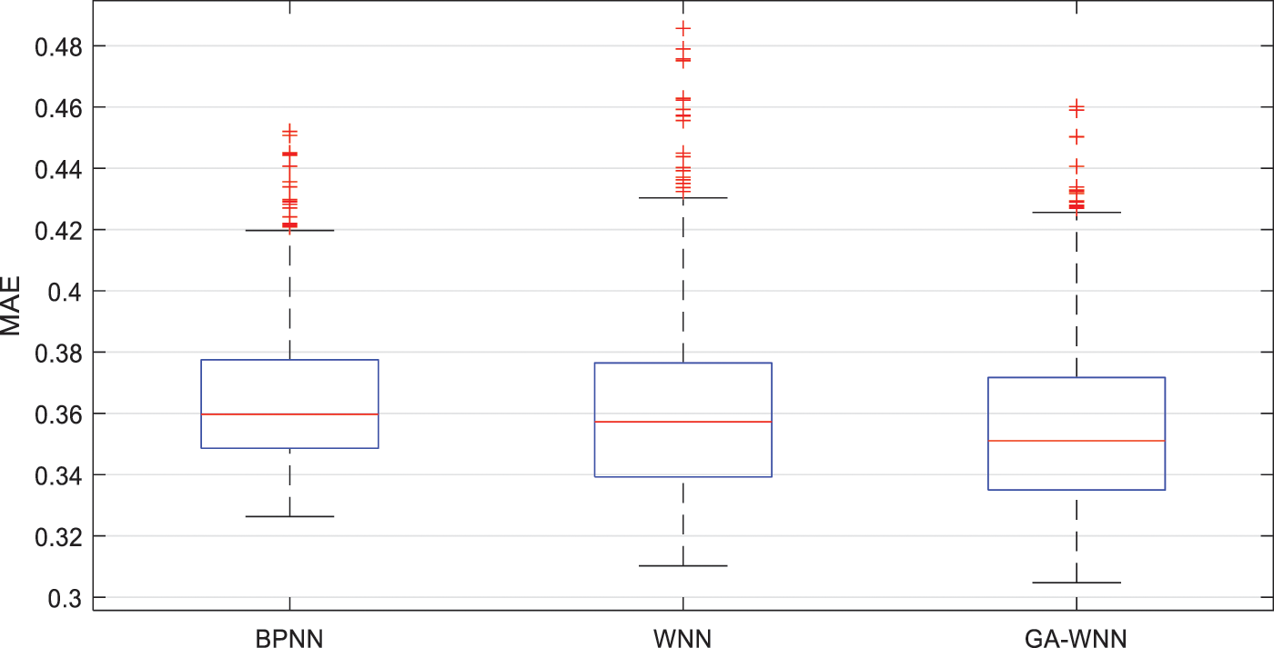
Figure 6: MAE histogram of the three network results

Fig. 7 shows R2 (coefficient of determination) distribution of the three networks results. R2 represents the degree of fitting between two samples. Generally, R2 is in the interval of 0 and 1. The closer the R2 is to 1, the better the fitting degree is; otherwise, the worse the fitting effect is. According to the results, R2 results of BPNN were mainly distributed in the range of 0.976 to 0.980, and average value was 0.9779. WNN sample results were distributed in the range of 0.978–0.982, and average value was 0.9802. GA-WNN was distributed in the range of 0.979–0.983 and average value was 0.9807. GA-WNN was also better than WNN and BP, and the R2 distribution results were more concentrated in a higher interval.

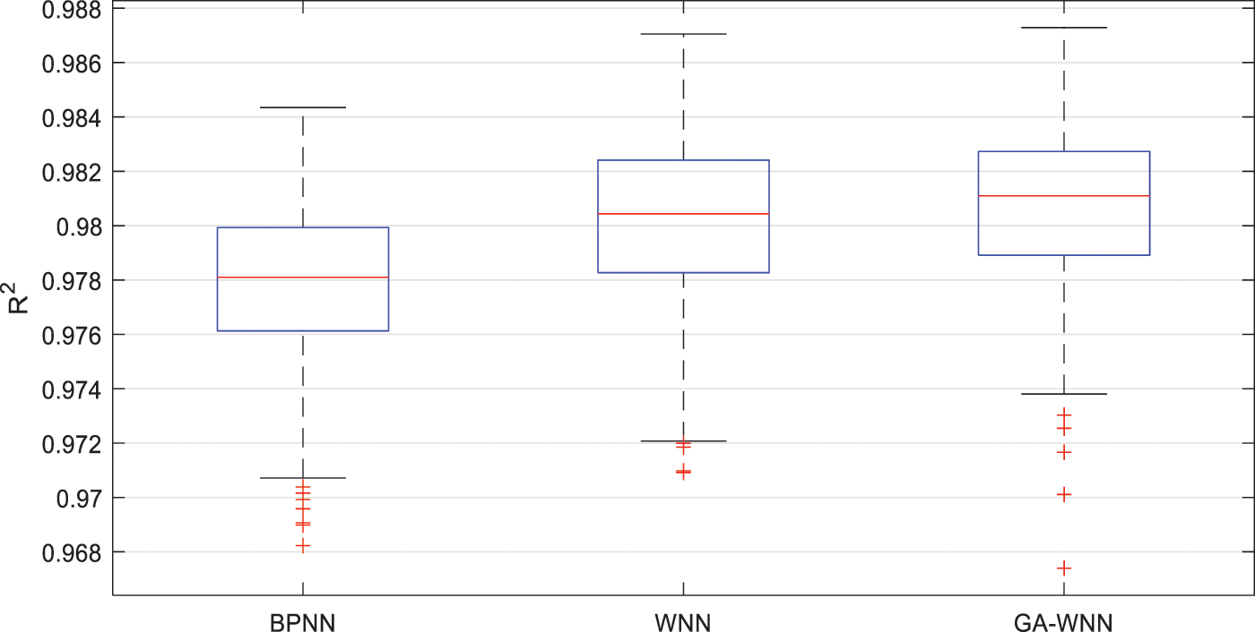
Figure 7: R2 histogram of the three network results

In Fig. 8, three neural networks were compared with the actual results in continuous time. It can be proved that GA-WNN had a strong prediction ability and more minor error compared with the others. The training cost is shown in Fig. 9. As the characteristics of each network were different, the comparison of the training cost was not significant. But the convergence trend of the actual error is meaningful. From Fig. 9, it seemed that GA-WNN had the fastest convergence speed, and complete convergence in 2 cycles, while the other networks achieved convergence in more than 6 epochs. It also verified the optimization effect of GA on network training by selecting the optimal weight.

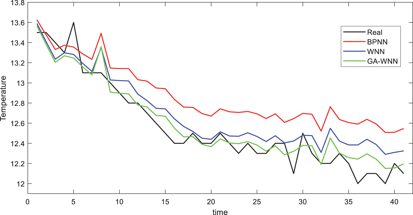
Figure 8: The temperature prediction results compared with the actual results. Time is the time point recorded by the sensor, each recording point interval is 5 min

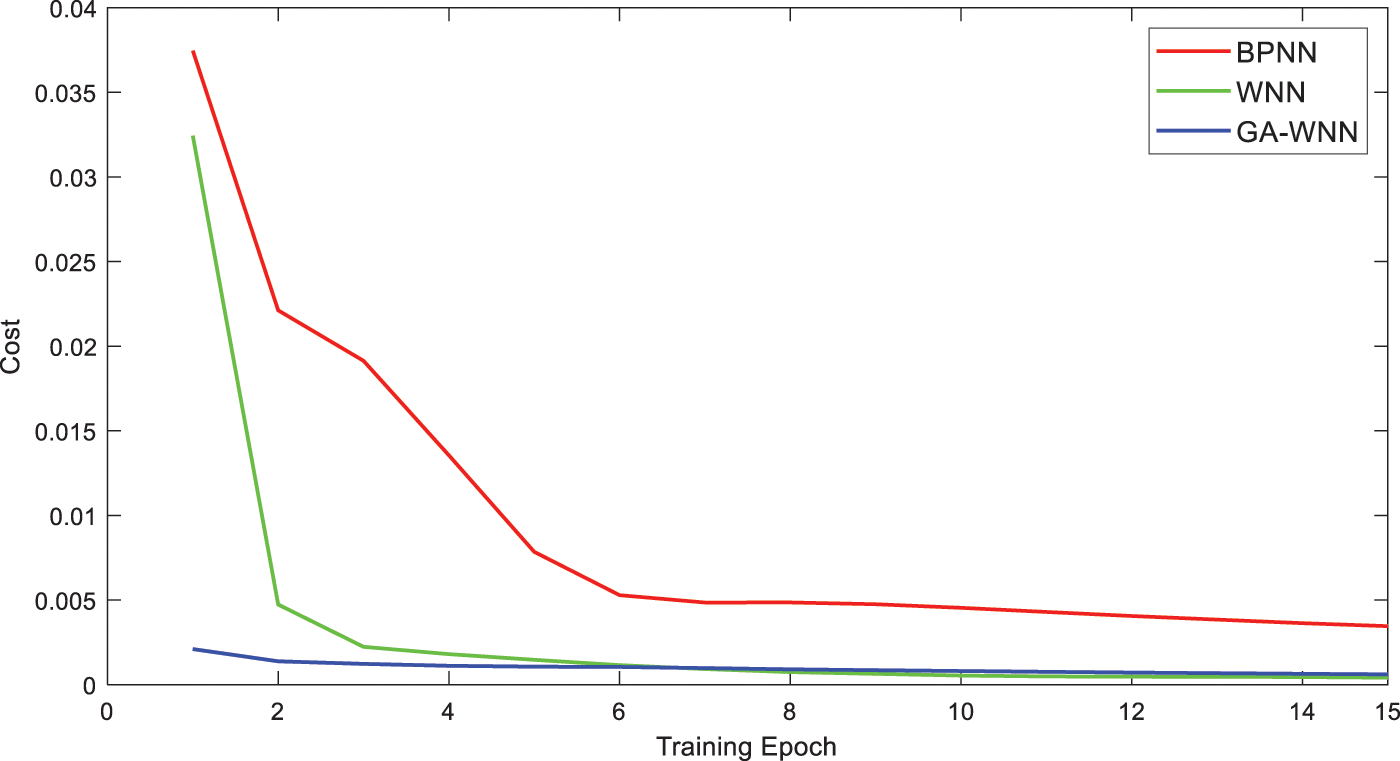
Figure 9: Error trend of the three neural networks in a single training process

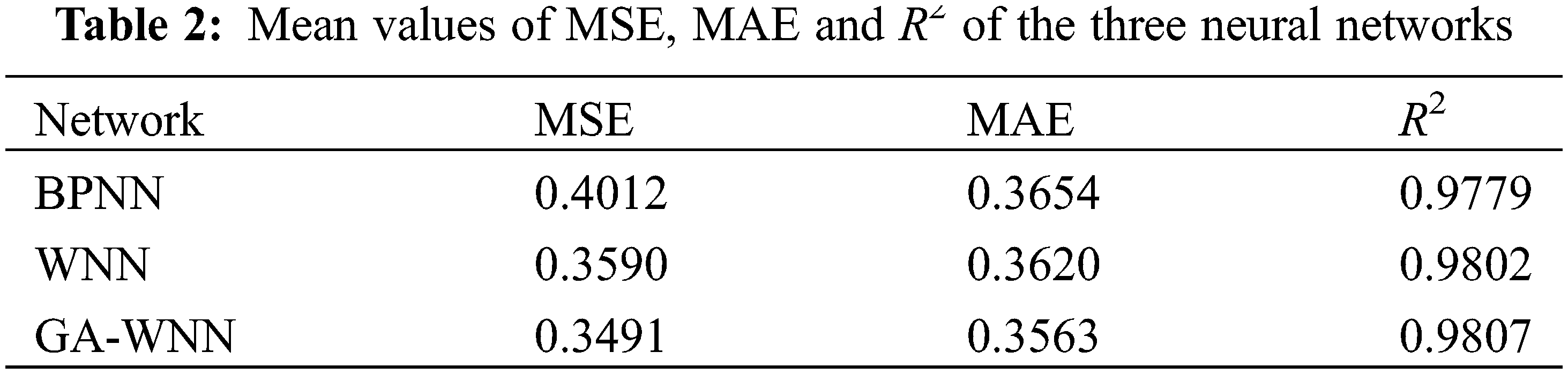
Table 2 shows the mean values of the three neural networks test results. Compared with BP, WNN had more advantages in prediction accuracy and kept most results within a better prediction level. GA further improved the stability of the prediction effect of WNN, enhanced the accuracy of convergence, reduced the prediction error, and accelerated the training speed. In all, GA-WNN showed a good performance in temperature prediction in a greenhouse, and a strong feasibility for the control application of the greenhouse.

4  Conclusion

In this paper, the ANN model was used to predict the temperature of the greenhouse, and a short-term greenhouse temperature prediction model based on GA-WNN was built. The model integrated the principle of wavelet transform and the characteristics of forward feedback network, which improved the model prediction and training speed. GA optimized the initial weight of WNN to avoid the uncertainty of the model training direction caused by the random weight initialization of the neural network, and improved the training speed. At the same time, it provided the optimal weight to ensure the stability and prediction accuracy of the subsequent model to avoid getting in local optimum problems. In the simulation, GA-WNN was compared with BPNN and WNN. The MSE, MAE and R2 results showed that GA-WNN had an excellent fitting ability and a strong model stability for greenhouse temperature modeling and prediction, and quickly completed the model training. Its prediction of the future temperature trend was conducive to the advance regulation of the greenhouse and ensured the stable operation of the greenhouse. The application and related research of the combination of wavelet neural network and genetic algorithm in the greenhouse is still lacking. We hope that this paper can better promote the application and research of WNN in the greenhouse and other fields.

Funding Statement: This research was funded by the National Natural Science Foundation of China (31901400, 61903351), Natural Science Foundation of Zhejiang (LQ20C130008, LY22F030009), and National Key Technologies Research & Development of China (2018YFB2101004).

Conflicts of Interest: The authors declare that they have no conflicts of interest to report regarding the present study.

References

 1.  Chahidi, L. O., Fossa, M., Priarone, A., Mechaqrane, A. (2021). Evaluation of supervised learning models in predicting greenhouse energy demand and production for intelligent and sustainable operations. Energies, 14 (19), 15. DOI 10.3390/en14196297. [Google Scholar] [CrossRef]

 2.  Achour, Y., Ouammi, A., Zejli, D. (2021). Technological progresses in modern sustainable greenhouses cultivation as the path towards precision agriculture. Renewable & Sustainable Energy Reviews, 147, 19. DOI 10.1016/j.rser.2021.111251. [Google Scholar] [CrossRef]

 3.  Tahery, D., Roshandel, R., Avami, A. (2021). An integrated dynamic model for evaluating the influence of ground to air heat transfer system on heating, cooling and CO2 supply in greenhouses: Considering crop transpiration. Renewable Energy, 173, 42–56. DOI 10.1016/j.renene.2021.03.120. [Google Scholar] [CrossRef]

 4.  Golzar, F., Heeren, N., Hellweg, S., Roshandel, R. (2018). A novel integrated framework to evaluate greenhouse energy demand and crop yield production. Renewable and Sustainable Energy Reviews, 96, 487–501. DOI 10.1016/j.rser.2018.06.046. [Google Scholar] [CrossRef]

 5.  Singh, M. C., Singh, J. P., Singh, K. G. (2018). Development of a microclimate model for prediction of temperatures inside a naturally ventilated greenhouse under cucumber crop in soilless media. Computers and Electronics in Agriculture, 154, 227–238. DOI 10.1016/j.compag.2018.08.044. [Google Scholar] [CrossRef]

 6.  Costantino, A., Comba, L., Sicardi, G., Bariani, M., Fabrizio, E. (2021). Energy performance and climate control in mechanically ventilated greenhouses: A dynamic modelling-based assessment and investigation. Applied Energy, 288, 116583. DOI 10.1016/j.apenergy.2021.116583. [Google Scholar] [CrossRef]

 7.  Gerasimov, D. N., Lyzlova, M. V. (2014). Adaptive control of microclimate in greenhouses. Journal of Computer and Systems Sciences International, 53 (6), 896–907. DOI 10.1134/S1064230714050074. [Google Scholar] [CrossRef]

 8.  Liu, R., Li, M., Guzmán, J. L., Rodríguez, F. (2021). A fast and practical one-dimensional transient model for greenhouse temperature and humidity. Computers and Electronics in Agriculture, 186, 106186. DOI 10.1016/j.compag.2021.106186. [Google Scholar] [CrossRef]

 9.  Malekpour Heydari, S., Aris, T. N. M., Yaakob, R., Hamdan, H. (2021). Data-driven forecasting and modeling of runoff flow to reduce flood risk using a novel hybrid wavelet-neural network based on feature extraction. Sustainability, 13 (20), 11537. DOI 10.3390/su132011537. [Google Scholar] [CrossRef]

10. Escamilla-Garcia, A., Soto-Zarazua, G. M., Toledano-Ayala, M., Rivas-Araiza, E., Gastelum-Barrios, A. (2020). Applications of artificial neural networks in greenhouse technology and overview for smart agriculture development. Applied Sciences, 10 (11), 43. DOI 10.3390/app10113835. [Google Scholar] [CrossRef]

11. Mahmood, F., Govindan, R., Bermak, A., Yang, D., Khadra, C. et al. (2021). Energy utilization assessment of a semi-closed greenhouse using data-driven model predictive control. Journal of Cleaner Production, 324, 18. DOI 10.1016/j.jclepro.2021.129172. [Google Scholar] [CrossRef]

12. Wang, L. N., Wang, B. R. (2020). Greenhouse microclimate environment adaptive control based on a wireless sensor network. International Journal of Agricultural and Biological Engineering, 13(3), 64–69. DOI 10.25165/j.ijabe.20201303.5027. [Google Scholar] [CrossRef]

13. Manonmani, A., Thyagarajan, T., Elango, M., Sutha, S. (2018). Modelling and control of greenhouse system using neural networks. Transactions of the Institute of Measurement and Control, 40 (3), 918–929. DOI 10.1177/0142331216670235. [Google Scholar] [CrossRef]

14. Gandhi, S. V., Thakker, M. T. (2019). Climate control of greenhouse system using neural predictive controller. 1st International Conference on Renewable Energy and Climate Change (REC), Ahmedabad, India: Springer-Verlag Singapore Pte, Ltd. [Google Scholar]

15. Jung, D. H., Kim, H. S., Jhin, C., Kim, H. J., Park, S. H. (2020). Time-serial analysis of deep neural network models for prediction of climatic conditions inside a greenhouse. Computers and Electronics in Agriculture, 173, 11. DOI 10.1016/j.compag.2020.105402. [Google Scholar] [CrossRef]

16. Hongkang, W., Li, L., Yong, W., Fanjia, M., Haihua, W. et al. (2018). Recurrent neural network model for prediction of microclimate in solar greenhouse. IFAC-PapersOnLine, 51 (17), 790–795. DOI 10.1016/j.ifacol.2018.08.099. [Google Scholar] [CrossRef]

17. Guo, Y., Zhao, H., Zhang, S., Wang, Y., Chow, D. (2021). Modeling and optimization of environment in agricultural greenhouses for improving cleaner and sustainable crop production. Journal of Cleaner Production, 285, 124843. DOI 10.1016/j.jclepro.2020.124843. [Google Scholar] [CrossRef]

18. Mahmood, F., Govindan, R., Al-Ansari, T. (2021). Predicting microclimate of a closed greenhouse using support vector machine regression. Computer Aided Chemical Engineering. Elsevier, Amsterdam, Netherlands. [Google Scholar]

19. Feng, Z. (2007). Comparison research and application of wavelet neural network and BP network (Master Thesis). Chengdu University of Technology, China. [Google Scholar]

20. Tian, Z. (2021). Approach for short-term traffic flow prediction based on empirical mode decomposition and combination model fusion. IEEE Transactions on Intelligent Transportation Systems, 22(9), 5566–5576. DOI 10.1109/TITS.2020.2987909. [Google Scholar] [CrossRef]

21. Feng, Y., Cui, N., Zhao, L., Hu, X., Gong, D. (2016). Comparison of ELM, GANN, WNN and empirical models for estimating reference evapotranspiration in humid region of Southwest China. Journal of Hydrology, 536, 376–383. DOI 10.1016/j.jhydrol.2016.02.053. [Google Scholar] [CrossRef]

22. Falamarzi, Y., Palizdan, N., Huang, Y. F., Lee, T. S. (2014). Estimating evapotranspiration from temperature and wind speed data using artificial and wavelet neural networks (WNNs). Agricultural Water Management, 140, 26–36. DOI 10.1016/j.agwat.2014.03.014. [Google Scholar] [CrossRef]

23. Nayak, P. C., Venkatesh, B., Krishna, B., Jain, S. K. (2013). Rainfall-runoff modeling using conceptual, data driven, and wavelet based computing approach. Journal of Hydrology, 493, 57–67. DOI 10.1016/j.jhydrol.2013.04.016. [Google Scholar] [CrossRef]

24. Sharma, V., Yang, D., Walsh, W., Reindl, T. (2016). Short term solar irradiance forecasting using a mixed wavelet neural network. Renewable Energy, 90, 481–492. DOI 10.1016/j.renene.2016.01.020. [Google Scholar] [CrossRef]

25. Jin, C., Mao, H. P., Chen, Y., Shi, Q., Wang, Q. R. et al. (2020). Engineering-oriented dynamic optimal control of a greenhouse environment using an improved genetic algorithm with engineering constraint rules. Computers and Electronics in Agriculture, 177, DOI 10.1016/j.compag.2020.105698. [Google Scholar] [CrossRef]

26. Yadav, R. K., Anubhav (2020). PSO-GA based hybrid with adam optimization for ANN training with application in medical diagnosis. Cognitive Systems Research, 64, 191–199. DOI 10.1016/j.cogsys.2020.08.011. [Google Scholar] [CrossRef]

27. Taghavi, M., Gharehghani, A., Nejad, F. B., Mirsalim, M. (2019). Developing a model to predict the start of combustion in HCCI engine using ANN-GA approach. Energy Conversion and Management, 195, 57–69. DOI 10.1016/j.enconman.2019.05.015. [Google Scholar] [CrossRef]

28. Panahi, F., Ahmed, A. N., Singh, V. P., Ehtearm, M., elshafie, A. et al. (2021). Predicting freshwater production in seawater greenhouses using hybrid artificial neural network models. Journal of Cleaner Production, 329, 129721. DOI 10.1016/j.jclepro.2021.129721. [Google Scholar] [CrossRef]

29. Tian, Z., Chen, H. (2021). A novel decomposition-ensemble prediction model for ultra-short-term wind speed. Energy Conversion and Management, 248, 114775. DOI 10.1016/j.enconman.2021.114775. [Google Scholar] [CrossRef]

30. Wang, L., Wang, B., Zhu, S. M. (2020). Multi-model adaptive fuzzy control system based on switch mechanism in a greenhouse. Applied Engineering in Agriculture,36(4), 549–556. DOI 10.13031/aea.13837. [Google Scholar] [CrossRef]

31. Wang, L. N., Wang, B. R. (2020). Construction of greenhouse environment temperature adaptive model based on parameter identification. Computers and Electronics in Agriculture, 174, 5. DOI 10.1016/j.compag.2020.105477. [Google Scholar] [CrossRef]

32. Chen, D. (2020). Application of wavelet analysis in speech signal processing. Information and Communication, 206(2), 20–21. DOI 10.3969/j.issn.1673-1131.2020.02.007. [Google Scholar] [CrossRef]

33. Du, W., Zhang, Q., Chen, Y., Ye, Z. (2021). An urban short-term traffic flow prediction model based on wavelet neural network with improved whale optimization algorithm. Sustainable Cities and Society, 69, 102858. DOI 10.1016/j.scs.2021.102858. [Google Scholar] [CrossRef]

34. Esen, H., Ozgen, F., Esen, M., Sengur, A. (2009). Artificial neural network and wavelet neural network approaches for modelling of a solar air heater. Expert Systems with Applications, 36(8), 11240–11248. DOI 10.1016/j.eswa.2009.02.073. [Google Scholar] [CrossRef]

35. Tian, Z. D. (2020). Network traffic prediction method based on wavelet transform and multiple models fusion. International Journal of Communication Systems, 33 (11), 25. DOI 10.1002/dac.4415. [Google Scholar] [CrossRef]

36. Ge, L. J., Li, Y. L., Yan, J., Wang, Y. Q., Zhang, N. (2021). Short-term load prediction of integrated energy system with wavelet neural network model based on improved particle swarm optimization and chaos optimization algorithm. Journal of Modern Power Systems and Clean Energy, 9(6), 1490–1499. DOI 10.35833/MPCE.2020.000647. [Google Scholar] [CrossRef]

37. Aly, H. H. H. (2020). A novel deep learning intelligent clustered hybrid models for wind speed and power forecasting. Energy, 213, 118773. DOI 10.1016/j.energy.2020.118773. [Google Scholar] [CrossRef]

38. Huang, Y., Li, C. (2021). Accurate heating, ventilation and air conditioning system load prediction for residential buildings using improved ant colony optimization and wavelet neural network. Journal of Building Engineering, 35, 101972. DOI 10.1016/j.jobe.2020.101972. [Google Scholar] [CrossRef]

39. Chen, Z. L., Zhao, C. J., Wu, H. R., Miao, Y. S. (2019). A water-saving irrigation decision-making model for greenhouse tomatoes based on genetic optimization T-S fuzzy neural network. Ksii Transactions on Internet and Information Systems, 13(6), 2925–2948. DOI 10.3837/tiis.2019.06.009. [Google Scholar] [CrossRef]

40. Mohamed, S., Hameed, I. A. (2018). A GA-based adaptive neuro-fuzzy controller for greenhouse climate control system. Alexandria Engineering Journal, 57(2), 773–779. DOI 10.1016/j.aej.2014.04.009. [Google Scholar] [CrossRef]

41. Oliveira, P. B. D., Pires, E. J. S., Cunha, J. B. (2017). Evolutionary and bio-inspired algorithms in greenhouse control: introduction, review and trends. 13th International Conference on Intelligent Environments (IE), Seoul, South Korea: Ios Press. [Google Scholar]

42. Wang, Z., Lu, F., He, H., Lu, Q., Wang, D. et al. (2015). Fine-scale estimation of carbon monoxide and fine particulate matter concentrations in proximity to a road intersection by using wavelet neural network with genetic algorithm. Atmospheric Environment, 104, 264–272. DOI 10.1016/j.atmosenv.2014.12.058. [Google Scholar] [CrossRef]

This work is licensed under a Creative Commons Attribution 4.0 International License, which permits unrestricted use, distribution, and reproduction in any medium, provided the original work is properly cited.