Phyton-International Journal of Experimental Botany

DOI: 10.32604/phyton.2022.017308

ARTICLE

A Study on Genotype-by-Environment Interaction Analysis for Agronomic Traits of Maize Genotypes Across Huang-Huai-Hai Region in China

Haiwang Yue1, Jianwei Wei1, Junliang Xie1, Shuping Chen1, Haicheng Peng1, Hongmei Cao2, Junzhou Bu1,* and Xuwen Jiang3,*

1Dryland Farming Institute, Hebei Academy of Agriculture and Forestry Sciences, Hebei Provincial Key Laboratory of Crops Drought Resistance Research, Hengshui, 053000, China
2Soil and Fertilizer Workstation of Hengshui Agriculture and Rural Bureau, Hengshui, 053000, China
3Maize Research Institute/College of Agronomy, Qingdao Agricultural University, Qingdao, 266109, China
*Corresponding Authors: Xuwen Jiang. Email: mjxw888@163.com; Junzhou Bu. Email: yanjiu1982@gmail.com
Received: 30 April 2021; Accepted: 24 June 2021

1  Introduction

Maize (Zea mays L.) is one of the most important food crops in the world, and it is also an important source of industrial raw materials and feed [1]. Since total maize production surpassed rice for the first time in 2012, maize had firmly occupied the position of China’s largest food crop [2]. Under the vast environmental conditions in China, breeders regard obtaining high-yield and stable hybrids as their primary goal. For this reason, scientific researchers must carry out multi-environment trials (METs) before the hybrids participate in national and provincial trials [3]. METs is an experimental system that evaluates specific genotypes under a series of different types of environmental conditions, which may be spatially separated (e.g., locations), time separated (different identification years), or a combination of space and time separation, our purpose was to evaluate the genotypes for specific environments and then make a recommended choice or an evaluation description of mega-environments [4]. METs requires the same experimental design in each environment (e.g., completely randomized block design with three replicates), the same genotypes (e.g., number and name of the genotypes), and the same agronomic practices (e.g., chemical spraying and weeding control) [5]. In this way, METs can effectively identify genotypes with small temporal variability or consistent trait performance among different environments [6].

In order to breed hybrids with wide adaptability and high stability, it is necessary to (1) systematically evaluate various germplasm resources and selected inbred lines in terms of yield, resistance, quality, etc., (2) obtain adaptation in different ecological regions, and basic data of adaptability, high yielding and stability in different ecological regions, and (3) comprehensively evaluate and screen out genotypes with excellent agronomic characteristics. Studies have shown that the performance of genotypic agronomic traits is not always stable and consistent in all environments. This is due to the existence of genotype by environment interaction effects (GEI), coupled with environment and genotype effects. Together, they constitute the influencing factors of phenotypic traits [7,8]. The environment (E) represents special natural conditions, such as rainfall, soil type, temperature, humidity, pests and diseases, etc., which lead to differences in the expression of genotypes. The phenotype expression changes of evaluated genotypes under different environmental conditions are called genotype (G) by environment (E) interaction (GEI) effects [9]. Due to the existence of GEI, it has caused confusion and reduced the efficiency of selection by breeders. It is very important to screen promising genotypes in different environments. GEI is one of the challenges faced by breeders. Therefore, from the perspective of plant breeding, improving crop genotypes requires a deep understanding and effective use [10].

The need for scientific modeling of GEI in the breeding process has led to the development of genotypes stability analysis. In order to better understand GEI, researchers have proposed various statistical analysis methods, Analysis of variance (ANOVA) analysis proposed from the beginning of the research, Yates et al. proposed the theory of joint regression analysis, which was widely promoted by Finlay et al. and Eberhardt et al. [11–14]. The stability variance proposed by Shukla and the yield stability parameter studied by Kang and the additive main effects and multiplicative interaction (AMMI) model proposed by Gauch et al. [15–17]. Among these statistical analyses, the AMMI model is undoubtedly one of the most widely used and most easily accepted methods, which combines analysis of variance and principal component analysis (PCA) to perform analysis with fixed effects in the METs analysis. In agricultural practice, people are often concerned about the grain yield trials, which has many genotypes tested in multiple environments, generally with 2–4 replications. Although grain yield is the most important characteristics of the crop itself, other agronomic traits are also common, such as plant height, ear height, ear length, and so on. If multiple agronomic traits are involved in METs, the AMMI model will analyze them one by one, not all of them [18]. Compared with its advantages, the AMMI model also has its own shortcomings. The AMMI model is a linear bilinear model, and future METs research will gradually reduce the dependence on the AMMI model, and more will rely on the linear mixed-effect model (LMM). This is because of the genotype estimates obtained through the best linear unbiased prediction (BLUP) is more accurate than the fixed effects model [19]. Olivoto et al. [20] combined the AMMI model with the BLUP method to provide two statistical analysis factors, WAASB (weighted average of absolute scores) and WAASBY (weighted average of WAASB and response variables), to evaluate genotypes based on the mean performance and stability (MPE) with different weights. If genotype selection is combined with grain yield and other agronomic traits, it may be more efficient, but how to accurately and effectively identify multiple traits has become a challenge for plant breeders. In view of this, Olivoto recently proposed a new strategy that shows how plant breeders can use the novel multi-trait genotype-ideotype distance index (MGIDI) to select genotypes in future breeding programs [21]. At the beginning of this century, Yan established a technique called “GGE biplot”, which is a form of mapping to show the main role of genotype (G) plus the genotype by environment interaction (GE) effect. The GGE biplot has an easy-to-identify graphic display to select high-yielding and stable genotypes, and can also distinguish the mega-environments, which is widely recognized by plant breeders [22]. The genotype by yield*trait (GYT) biplot method is a new analysis approach for multi-traits evaluation in recent years. This method used GGE biplot analysis to verify the evaluated genotypes and can also determine the strengths and weaknesses of each genotype [23].

The Huang-huai-hai plain is the largest region of summer maize planting in China, accounting for about one-third of the national maize output. The average maize yield in this area is still relatively low, mainly due to the farming system, abnormal weather conditions, pests and diseases, etc. The proportion of maize in China’s economic development is unmatched by other crops. How to improve the grain yield and quality of maize hybrids to meet the increasing living requirements of the people has always been the direction of the efforts of maize scientists in China [24]. Therefore, the purposes of this research were to: (i) verify the potential of the MGIDI index in future research using the real data across 24 environments in 2018–2019; (ii) present the genotype stability evaluation system for weighting the different agronomic traits and stability; (iii) evaluate the genotypes with multiple traits through genotype by yield*trait (GYT) biplot and selection indexes (SI); (iv) compare the genotypes ranking with the previously recognized parameter indicators, and analyze the evaluated traits using the Spearman’s correlation matrix.

2  Materials and Methods

2.1 Plant Materials and Field Evaluation

In this study, a total of 28 promising maize genotypes were planted in 24 locations across 6 provinces with three replications based on a randomized complete block design (RCBD) for two consecutive years (2018–2019). The description of the hybrids and locations used in this study are shown in Tab. 1. The row length and width of each plot were 6.7 meters and 3 meters respectively; the row spacing was 0.6 meters, with a final seedling population density of 75,000 plants/ha. During the experiment, all the agronomic practices, such as irrigation, fertilization application, chemical control of weeds and pesticides, were carried out at an appropriate time.

2.2 Data Collection

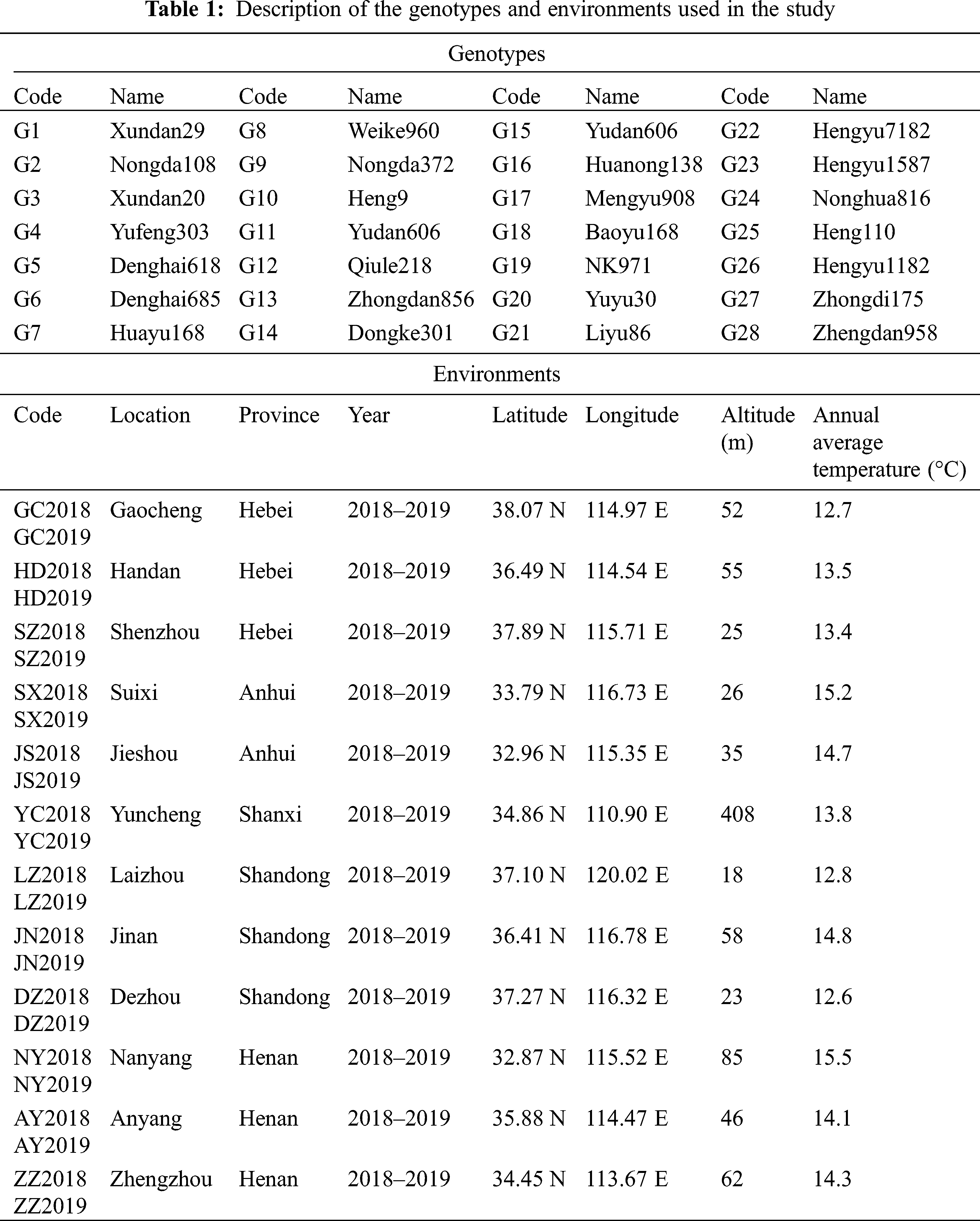
The 12 agronomic traits measured in this study were collected from the middle three rows of each plot. Grain yield (GY, t/ha) was manually harvested from the middle three rows, adjusting the moisture to 14% and converting the unit to tons per hectare; growth period (GP, d), investigating the number of days from emergence to maturity in each plot; grain moisture content (GMC, %), measured from each plant at each plot; plant height (PH, cm), measured from the base of the root to the top of the tassel; ear height (EH, cm), measured from the base of the root to the stalk of the ear; ear length (EL, cm), measured from the line up 10 ears, and dividing the data obtained by 10; ear diameter (ED, cm), determined by arranging 10 ears vertically, and dividing the data obtained by 10; ear row (ER), counting the total number of rows in each ear; bare tip length (BTL, cm), measured from the top part with no grains (if any) to the part with grains; grain weight per ear (GWE, g), 100-seed weight (HSW, g), lodging rate (LR, %).

2.3 Statistical Analysis

2.3.1 AMMI Model

For situations where complex GEI structures are observed, AMMI analysis can be used to obtain a more accurate estimate of Yger, and the formula is as follows: Yger=μ+αg+βe+∑n⁡λnγgnδen+ρge+εger where Yger represents the yield of genotype g in environment e for replicate r; μ represents the grand mean, αg and βe represent the genotypes and environments deviation from μ, respectively; λn represent the singular value of principal component axis (PCA) n; γgn and δen are the eigenvector values of genotype g and environment e of axis n, respectively; ρge represents the residual of AMMI model; and εger represents the error [25].

2.3.2 The Best Linear Unbiased Prediction (BLUP) Model for Multi-Environment Trials (METs)

The simplest and most well-known linear model with interactions used to analyze the data of multi-environment trials, and the formula is as follows: yijk=μ+αi+τj+ατij+γjk+εijk where yijk is the agronomic trait observed in the kth block of the ith genotype in the jth environment; μ represents the grand mean; αi and τj are the effect of the ith genotype and jth environment, respectively; ατij is the interaction effect of the ith genotype with the jth environment; γjk is the effect of the kth block within the jth environment; εijk is the random error [26].

2.3.3 Combining of AMMI Model and BLUP Method

In order to better combine the functions of AMMI model and BLUP techniques, we adopted the genotype stability evaluation system proposed by Olivoto et al. [4]. The stability index of each genotype in METs called WAASB index was calculated by the following formula: WAASBi=∑k=1p⁡|IPCAik×EPk|∑k=1p⁡EPk where WAASBi is the weighted average of absolute scores of the ith genotype; IPCAik is the score of the ith genotype in the kth interaction principal component axis (IPCA). In the usage of the traditional AMMI model, singular value decomposition (SVD) is used to decompose the matrix with additive model residuals into k IPCAs, and scores are obtained by the SVD of the GEI effects obtained in the linear mixed effects model, and EPk is the amount of the variance explained by the kth IPCA. Genotypes with a lower WAASB value are considered to be more stable genotypes; on the contrary, a genotype with a higher WAASB value is generally considered to be unstable [20]. By using the WAASBY index while performing mean performance and stability (MPE), it allows weighting between the mean performance Y and stability index (WAASB), as shown below: WAASBYi=(rYi×θY)+(rWi×θs)θY+θs where WAASBYi is the superiority index with different weights between mean performance and stability for the ith genotype; θY and θs are the weights for mean performance and stability, respectively; rYi and rWi are the recalculated values of the rth genotype for mean performance and WAASB, respectively, as shown below: rYi=100−0Ymax−Ymin×(Yi−Ymax)+100 rWg=0−100Wmax−Wmin×(Wi−Wmax)+0 where Yi and Wg are the mean performance and WAASB values of the ith genotype, respectively [25].

2.3.4 The Calculation of Multi-Trait Stability Index (MTSI)

The only difference from the multi-trait genotype-ideotype distance index (MGIDI) is that the Fgp matrix affected by factor analysis (FA) in MTSI contains WAASBY values, and its calculation formula is as follows:

In the formula, MTSIi represents the multi-trait stability index of the ith genotype, Fij represents the jth score for the ith genotype, and Fj represents the jth score of the ideal genotype. MTSI is used for genotype evaluation and selection based on mean performance and stability (MPE). The genotype with the lowest MTSI value is closer to ideology, and its MPE is high for all the analyzed traits [27].

2.3.5 Smith-Hazel Index

The classic multi-trait stability evaluation method Smith-Hazel (SH) index calculation formula is as follows:

Among them, b and w represent the vectors of index coefficient and economic weight, respectively; P and G represent the phenotype and genetic covariance matrix, respectively [28,29].

2.3.6 Multi-Trait Index Based on Factor Analysis and Genotype-Ideotype Distance (FAI-BLUP Index)

After determining the ideotype, estimate the distance between the ideotype and each genotype, and then convert it into a spatial probability, so that the genotypes can be ranked. The calculation formula of FAI-BLUP index is as follows: Pij=1dij∑i=1; j=1i=n; j=m1dij where Pij represents the probability that the ith genotype (i = 1, 2, …, n) is similar to the jth genotype (j = 1, 2, …, m); dij represents the genotype-ideotype distance from the ith genotype to the jth ideotype according to the standardized average Euclidean distance [30].

2.3.7 The Multi-Trait Genotype-Ideotype Distance Index (MGIDI)

According to the multi-trait genotype-ideological distance index (MGIDI) proposed by Olivoto et al. [21], it ranks genotypes based on multiple traits. The entire calculation process of MGIDI was divided into the following four steps. First, using the following formula to rescale value for the jth agronomic trait on the ith genotype (rXij): rXij=ηnj−\phinjη0j−\phi0j×(θij−η0j)+ηnj where ηnj and φnj represent the new maximum and minimum values of the jth agronomic trait after rescaling, respectively; η0j and φ0j represent the original maximum and minimum values of the jth agronomic trait, respectively; θij represent the original value of the ith genotype in the jth agronomic trait. Choose the values for ηnj and φnj according to the following criteria: when you want to obtain a trait with positive gain, you should use φnj = 0 and ηnj = 100; on the contrary, when you want to obtain a trait with negative gain, φnj = 100 and ηnj = 0 should be used. In this study, the agronomic traits GY, EL, ED, ER, GWE and HSW belong to positive desired gains, and the agronomic traits GP, GMC, PH, EH, BTL and LR belong to negative desired gains.

In the second step, the problem of dimensionality reduction of data and relational structure was solved by performing factor analysis (FA). The calculation of factor analysis relies on the following formula:

In the formula, γij represents the scores of the ith genotype in the jth factor (i = 1, 2,…, t; j = 1, 2,…, f), where t and f represent the number of genotypes and factors, respectively, and γj represents the jth scores for the ideotype. The genotypes with the lower MGIDI values are closer to the ideal genotype than other genotypes and exhibits all the desired values for the measured agronomic traits.

MTSI takes advantage of the weight between average performance and stability, and therefore selects genotypes that are both stable and have a high-performance. If the weights of all traits in the MTSI are completely assigned to the average performance, then the MTSI will become the MGIDI index. It should be noted that MGIDI is used to rank genotypes based on multiple traits, but does not consider the stability of genotypes.

2.3.8 Genotype by Yield × Trait (GYT) Biplot

The GYT biplot used the theory proposed by Yan et al. [23]. For the GYT biplot analysis, the agronomic trait grain yield was taken as the basic variable (yield). Based on the standardized GYT, the superiority index (SI) that integrates all yield-traits was calculated [31].

2.3.9 Relationship Between Stability Measures for Grain Yield

In this section, indexes WAAS and WAASY (consider a fixed-effect model), and compare the indicators WAASB and WAASBY (considering the mixed-effect model) with the following 13 AMMI-derived stability indexes in terms of genotype ranking, namely: (1) Absolute values of the first and principal component axis, respectively, PC1 and PC2; (2) AMMI stability value, ASV [5]; (3) Sums of the absolute value of the IPCA scores, SIPC; (4) Average of the squared eigenvector values, EV; (5) Absolute values of the relative contributions of the IPCAs to the interaction, ZA; (6) Harmonic mean of the relative performance of the genotypic values, HMRPGV; (7) Coefficient of variation, CV; (8) Adjusted coefficient of variation, ACV; (9) Power law residuals, POLAR; (10) Annichiarrico’s genotypic confidence index for all, favorable and unfavorable environments, respectively, Wi_g, Wi_f and Wi_u; (11) Wricke’s ecovalence, Ecoval; (12) Deviations from the joint-regression analysis, Sij; (13) The ssi are the simultaneous selection indexes using AMMI-derived stability indexes. Calculate the ranking of genotypes based on the concept of each indicator. Principal component analysis (PCA) was computed to explore the relationships between the research indicators; then, it will be displayed in the form of a loading biplot.

2.3.10 Statistical Analysis Software

All statistical analysis were performed based on the R version 4.0.3 software with the “metan” version v1.12.0 package, and the packages used by the principal component analysis with biplot are “FactoMineR” verson 2.4, “ggplot2” version 3.3.4 and “factoextra” version 1.0.7. The functions including gamem( ), mtsi( ), mgidi( ), Smith_Hazel( ), fai_blup( ), waas( ), waasb( ), gytb( ) and AMMI_indexes( ) were used in this study [32].

3  Results

3.1 Variance Components of the 12 Agronomic Traits and Factors Description

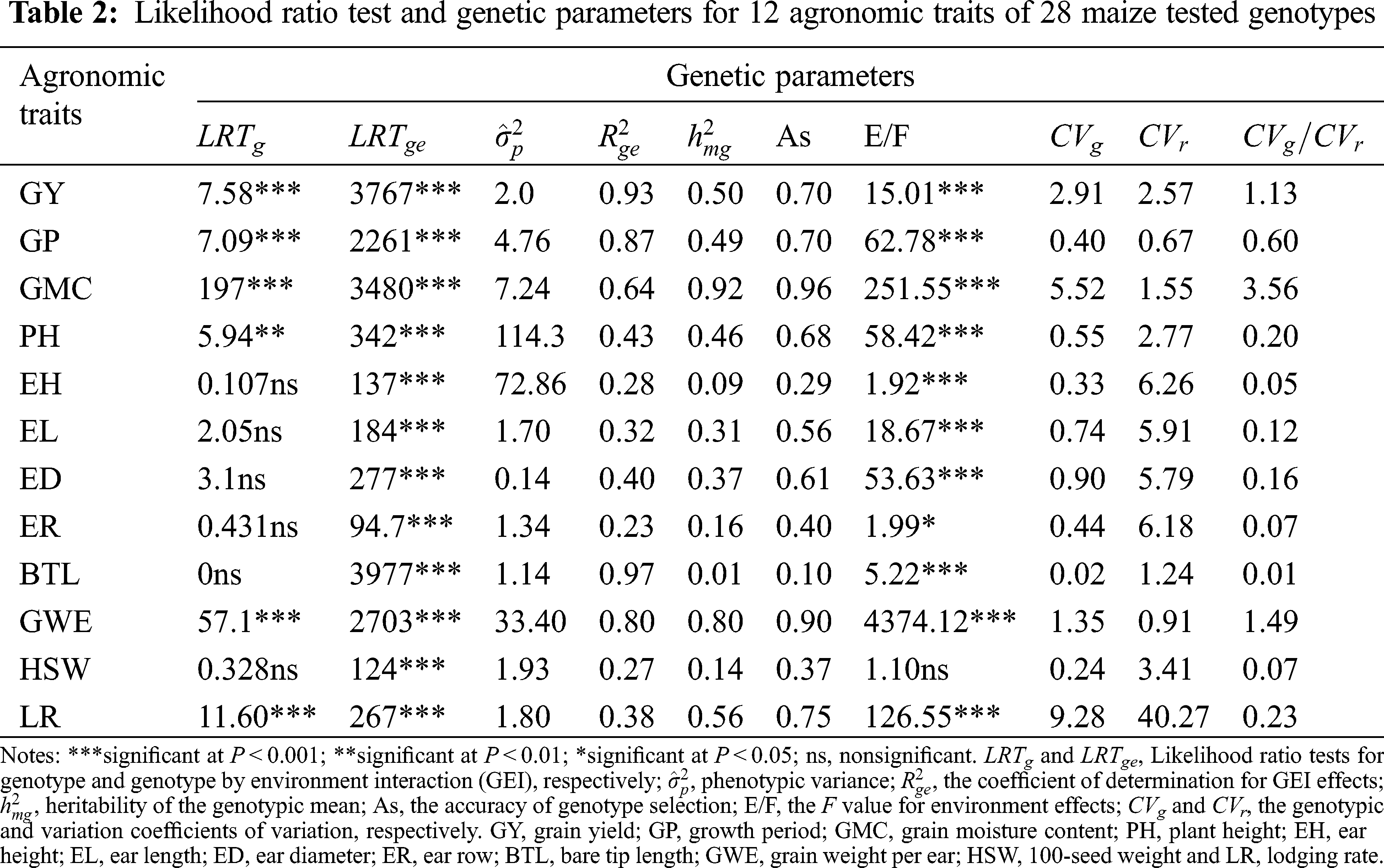
The genotype had highly significant effects (P < 0.001 and P < 0.01) for the maize agronomic traits GY, GP, GMC, PH, GWE and LR, and the GEI revealed a highly effect (P < 0.001) for all traits according to the likelihood ratio (Tab. 2). The environment effect was highly significant for all evaluated traits except for HSW. The accuracy of genotype selection (AS) for 12 analyzed traits ranged from 0.10 (BTL) to 0.96 (GMC). High values of the coefficient of determination for GEI effects ( Rge2 ) were observed for GY, GP, GMC, BTL and GWE, indicating that the GEI variance occupies an important part of the phenotypic variance component.

3.2 Loadings and Factors Description for MGIDI

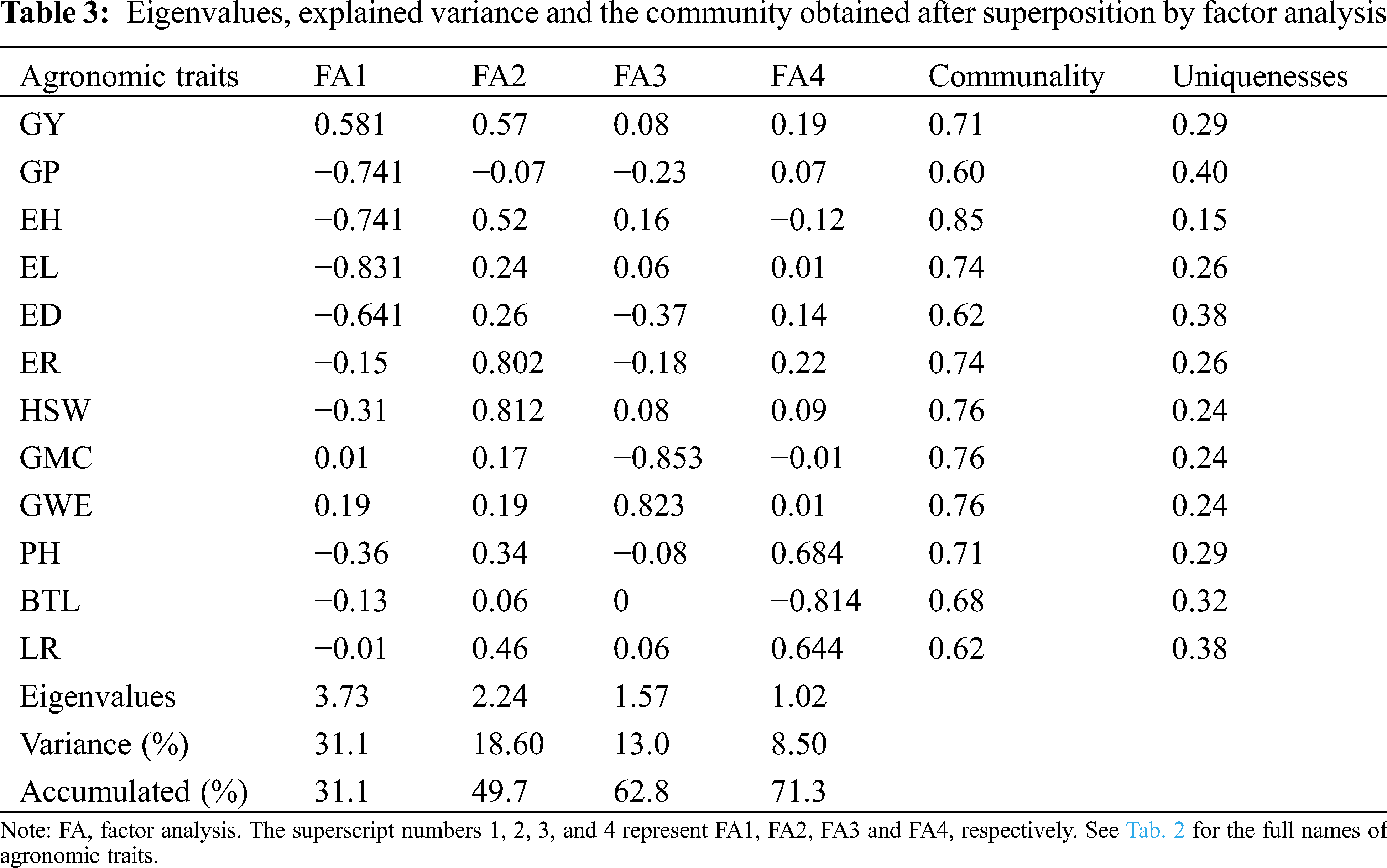
According to 71.28% of the total variation of the explained traits, we retained the top 4 main components (Tab. 3). After layers of accumulation, the average communality was 0.71 (the maximum value was 0.85, the minimum value was 0.62), which means that factors (FA) can explain a large part of the variance of each variable. In this study, the 12 evaluated traits were divided into 4 factors. GY, GP, EH, EL and ED belonged to FA1; FA2 characteristics included ER and HSW; FA3 included traits GMC and GWE. The remaining three traits PH, BTL and LR were classified as FA4.

3.3 Genotypes Selected by Different Evaluation Methods

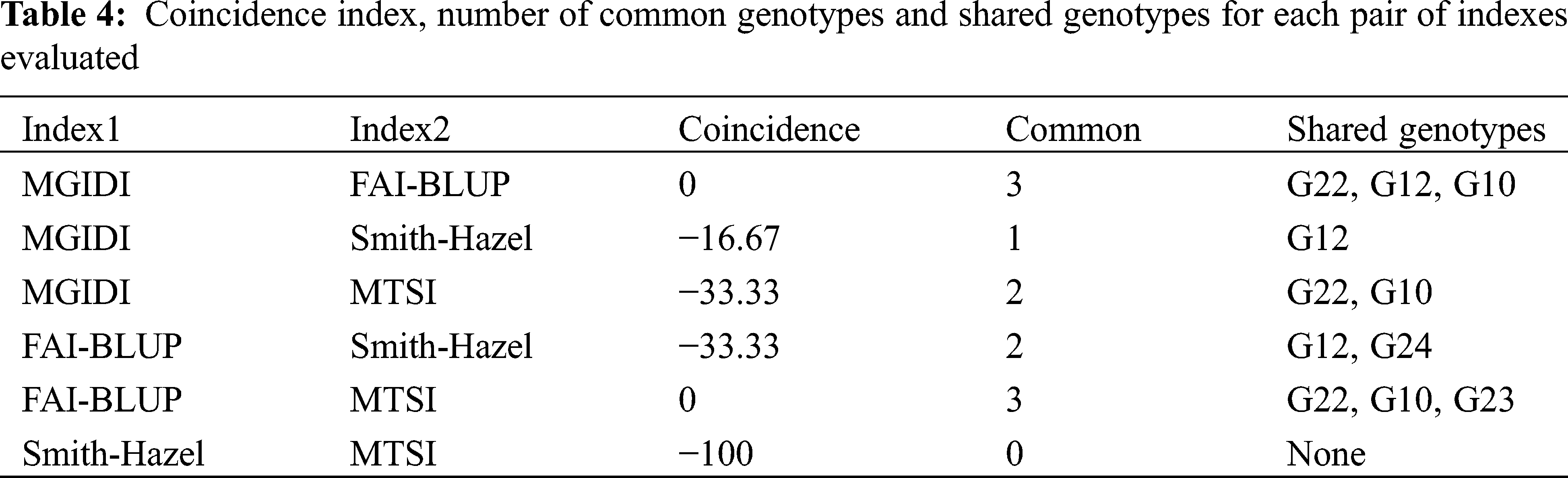
Assuming that the selection intensity was controlled at 15%, we can screen out different genotypes through different evaluation methods (Fig. 1). Genotypes G21, G22, G23, G24, G10 and G12 were selected by FAI-BLUP (Fig. 1a). The genotypes selected according to the MGIDI index were G22, G12, G10 and G1 (Fig. 1b), Through the MGIDI index, the genotypes G15, G4 and G26 were very close to the red cutting point (the red circle represents the number of genotypes selected based on the selection pressure), which means that these genotypes are expected to have an excellent phenotype. Genotypes 23, 22, 10, 2 and 12, 24, 11, 14 were selected by the MTSI and SHindexes (Figs. 1c and 1d), respectively. The genotypes G22, G10 and G12 were selected more times, followed by G 23 and G24 (Fig. 1e, Tab. 4), implying that these two genotypes performed better and stable in different environments.

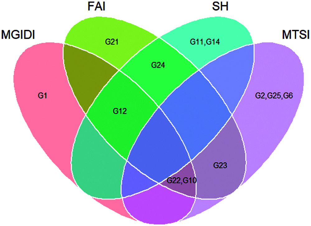
Figure 1: Genotype ranking for the FAI-BLUP (a), Multi-trait genotype ideotype distance index (MGIDI) (b), Smith-Hazel index (c), Multi-trait stability index (MTSI) (d), and Venn plot (e)

3.4 Combining Features of AMMI and BLUP Techniques

Fig. 2 showed the combined interpretation for mean performance and stability of the 12 agronomic evaluated traits. In the GY × WAASB biplot, the abscissa represents the performance of grain yield, and the ordinate represents the WAASB value. WAASB achieves the purpose of quantifying stability by considering all possible interaction principal component axis values. The biplot is divided into four quadrants by lines perpendicular to the abscissa and ordinate. The genotypes within Quadrants I and II are considered to be less stable. Different traits within Quadrants III and IV have different meanings. Genotypes within Quadrants IV (for GY, HSW, EL, ED, ER and GWE which higher values are desired) and III (for GP, GMC, PH, EH, BTL and LR which lower values are better) are assumed to be desirable.

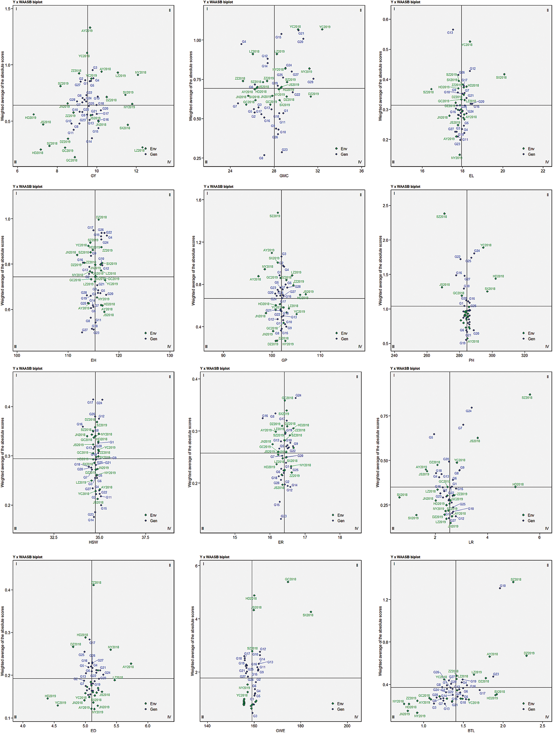
Figure 2: AMMI biplot based on the mean performance and stability of each trait. The X-axis shows the observed value of different traits and the Y-axis represents the WAASB index

Regarding the grain yield and stability performance for environments, located in the quadrant I, it shows the lower performance below the average yield, and plays a maximum role in genotype and environment interaction. The environments in the second quadrant is the same as that in the first quadrant, which means that it plays a greater role in GEI, and the difference is that the trait performance is still good. So the environments in the second quadrant deserve special attention because they provide above-average trait performance and high ability to distinguish genotypes. The environments in quadrant III have a low yield performance, and given their low WAASB values, these environments have a weaker ability to distinguish genotypes. The environment in the last quadrant has higher grain yield performance and lower WAASB value.

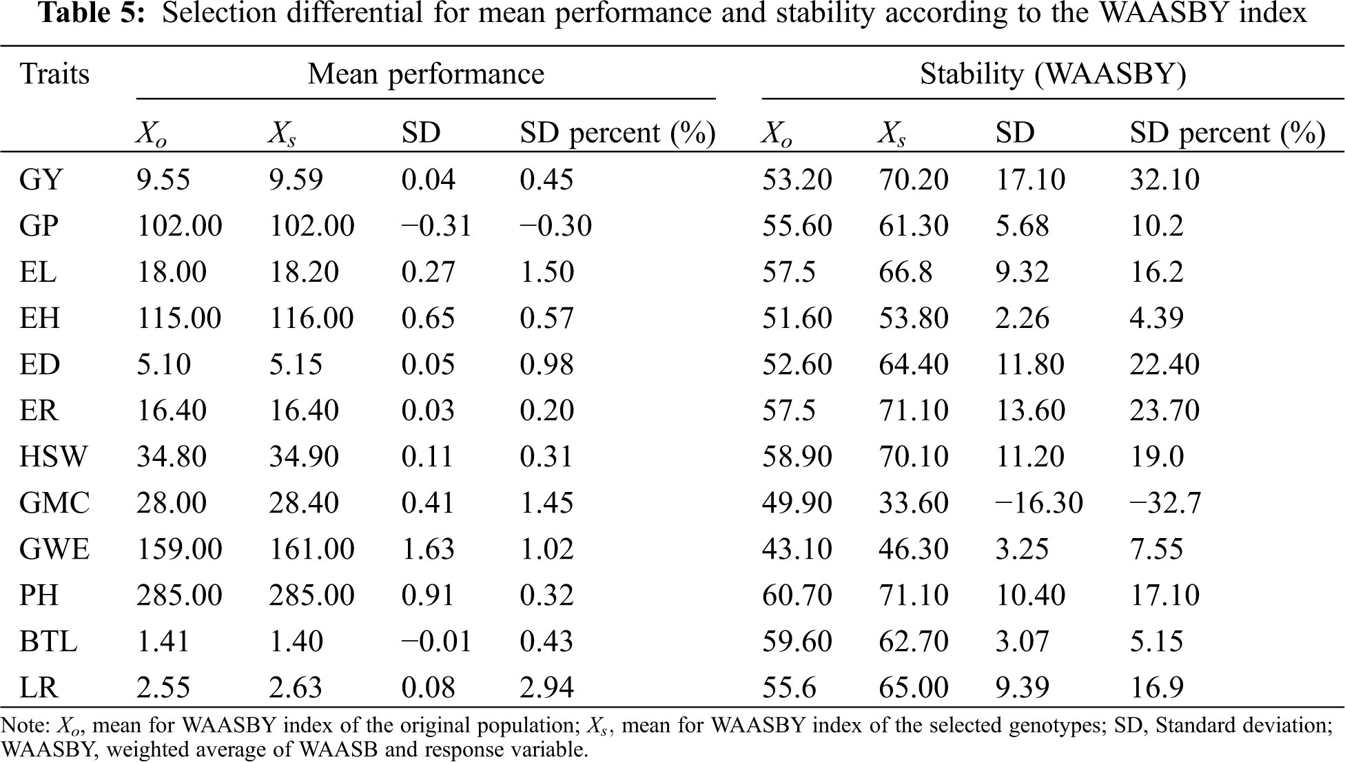
Among the 12 agronomic traits evaluated, the observed values of the selected genotypes were all higher than the average except for GP and BTL, and the SD percentage of the trait value and average performance of the selected genotypes was −0.17% for GP and −2.94 for LR. This result can bring some enlightenment to maize breeding. The maize growth period and bald tip are two agronomic traits that breeders try to control. Regarding the WAASBY index, except for GMC, positive selection differences were observed in all other agronomic traits (4.39% for EH ≤ selection difference ≤ 32.1% for GP), which indicated that the selected genotypes were more stable (Tab. 5).

The ranking of genotypes depending on the number of PCAs used to estimate the WAASB was shown in Fig. 3a, and ranking of genotypes considering the WAASB/GY ratio was shown in Fig. 3b. The left and right sides of Fig. 3 give more weight to genotype stability and grain yield, respectively. Genotype groups with similar stability capabilities can be easily divided into 4 groups by genotype codes of different colors. The genotypes in the first group, such as G14 and G15, have the best overall stability and yield performance. These genotypes are highly productive and broadly adaptable because they maintain a similar independence in terms of average yield and stability weights. Because they have similar ranking independence given weight for average performance and stability, these genotypes have higher level of productivity and wider adaptability. The genotypes in the second group have poor stability but higher yields. The representative genotypes here are G3, G4 and G5. The genotypes in the third group are opposite to those in the second group, with higher stability but lower yield. G8, G11 and G12 are representatives of this group. The genotypes in the fourth group, have the characteristics of poor stability and poorly productive, especially G1, G2, G3 and G27.

Figure 3: The heatmap shows the ranking of 28 maize genotypes according to the amount of IPCA scores used to compute the WAASB index (a) and different weights for yielding and stability used in this study (b)

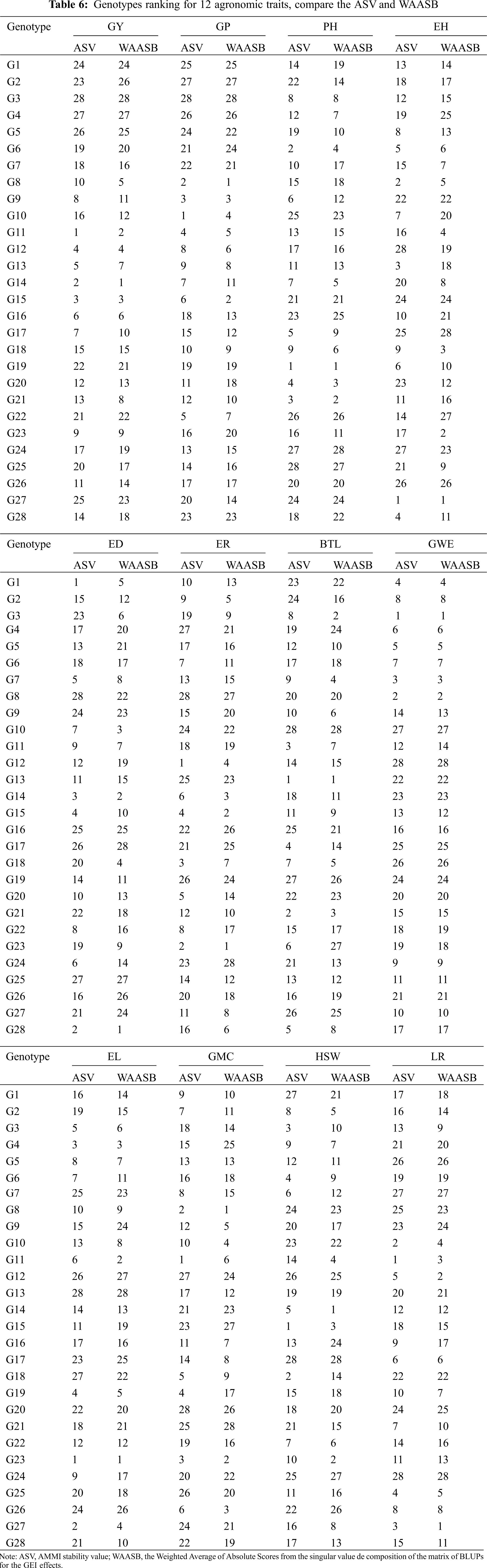
3.5 Comparison of Genotype Ranking Based on Stability Index ASV and WAASB

In this study, we introduced a new evaluation method for genotype stability in multi-environment trials (METs), the weighted average of absolute scores from the singular value decomposition of the matrix of BLUPs for the GEI effects (WAASB). The ranking of genotypes was very similar or the same as the traditional evaluation method AMMI stability value (ASV) (Tab. 6). As the degree of METs and the complexity of GEI increased, GEI in the form of being retained in a large number of IPCA in AMMI analysis tends to be captured in the final IPCAs. Thus, the WAASB index is very promising for obtaining a convincing genotype evaluation by quantifying genotype stability in future studies.

3.6 Genotype by Yield*Trait (GYT) Biplot

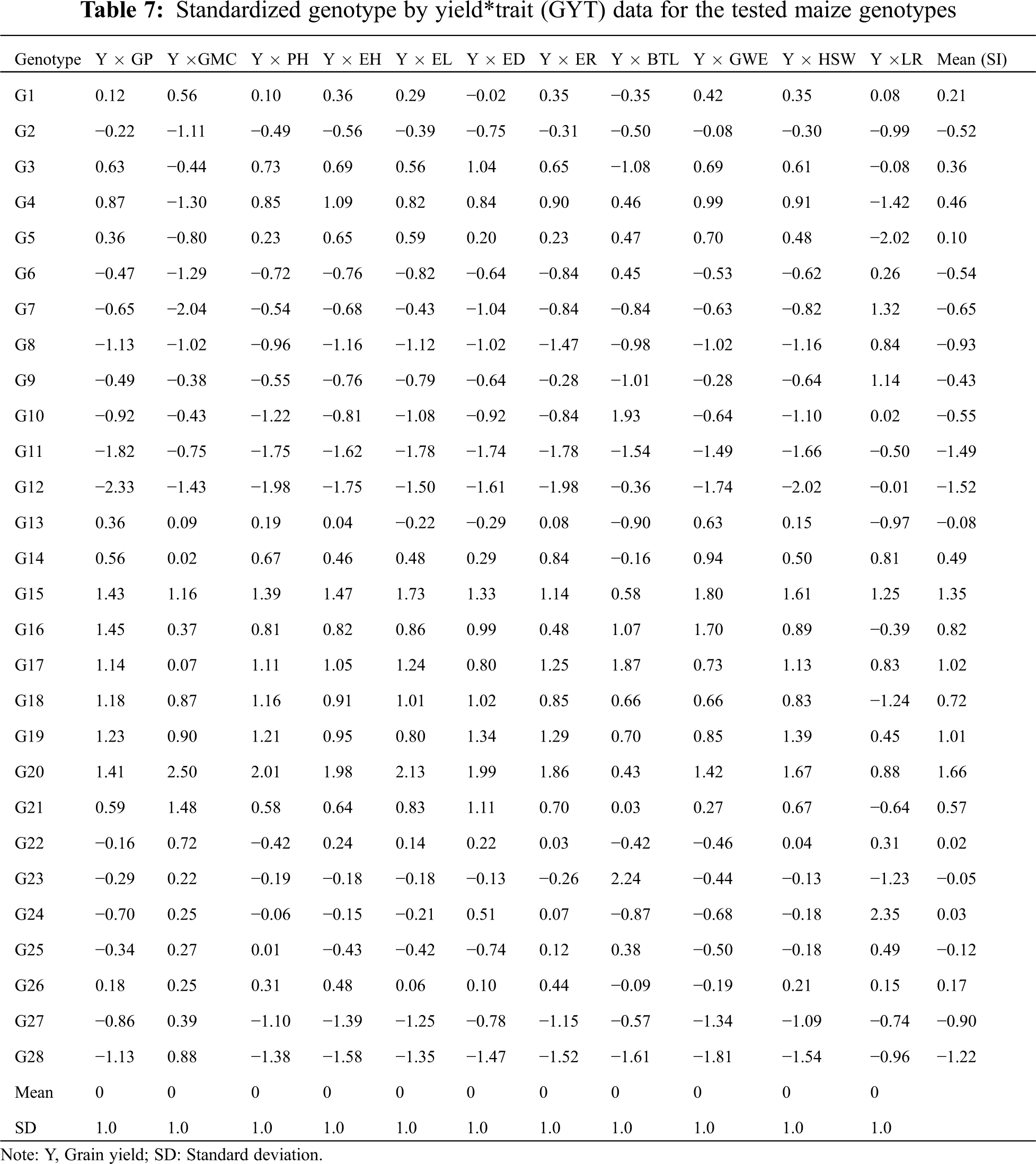
The GYT biplot, which combines grain yield and any other agronomic traits, can be used to evaluate how grain yield is combined with such trait. Thus, the use of GYT biplot technology can determine when the value of any genotype trait was low, and then the grain yield was high. The reverse is also true, and whether the results were affected by this combination or whether the ranking changes accordingly. As a result, when agronomic traits and grain yield values are input in combination, the data changes with the genotype ranking. Therefore, it is always desirable to have a larger value in the GYT table. The values of 28 maize genotypes in 24 different environments over 2 years are listed in Tab. 7. The superiority index (SI) ranks genotypes by all traits, among which the higher SI values were defined as the best genotypes. According to Fig. 4, the genotypes G20, G15, G16, G19 and G17 had the highest grain yield; on the contrary, G28, G11 and G12 were classified as the worst genotypes. According to the principle introduced in the GYT biplot method, the relationship between the grain yield and agronomic traits combinations in Fig. 4 can be further observed. In the GYT biplot, except for Y*LR, in view of the acute-angle relationship between the vectors, all yield-trait combinations showed a positive correlation. The grain yield-agronomic trait combination provided a very meaningful way to rank genotypes through graphs. The same relationship can be clearly seen through the GYT biplot; for example, the lower correlation value and the acute angle within the vectors between Y*GP, Y*EH, Y*HSW, Y*PH, Y*ER, Y*ED and Y*EL.

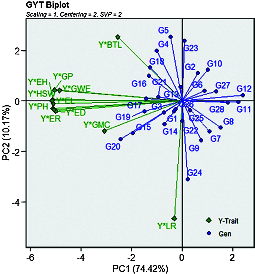
Figure 4: The associations of the combinations between grain yield and other traits based on the genotype by yield * trait (GYT) biplot

3.7 Correlation Between Different Agronomic Traits

The spearman’s correlation matrix among the 12 agronomic traits and the significance between the traits was presented in Fig. 5. A high-magnitude positive correlation was observed between GWE, ED, EL, PH and GY, while a negative significance was reached between LR, BTL GP and GY, suggesting that the above agronomic traits have positive and negative effects on grain yield, respectively. Agronomic traits PH, EH, ER, ED, EL, LR and HSW reached a significant positive correlation with each other. However, PH, ED and BTL, GWE and GMC, LR and GP reached a significant negative correlation.

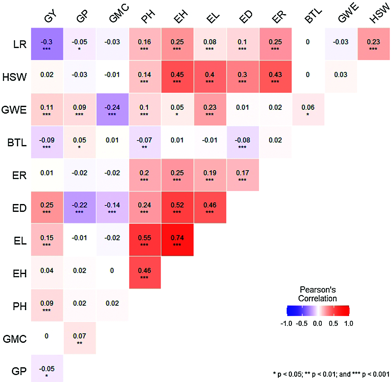
Figure 5: The correlation heat map among the 12 different agronomic traits. *, **, and *** represents significance at 0.05, 0.01 and 0.001, respectively

3.8 Correspondence Among the Stability Indexes

The loading biplot obtained by principal component analysis (PCA) considering the correlation matrix with grain yield and stability statistics indexes was presented in Fig. 6. The first two PCAs explained accounted for 74% of the GEI variance. Except for EV, SIPC, ACV, POLAR, CV and PC1, all other stability indexes vectors were very long, which indicated that they were well expressed in the factor plane. It can also be seen from Fig. 6 that the stability indexes used for evaluation could be divided into left and right parts according to the middle dotted line. The angles between their vectors of the left part was less than 90°, indicating that these indexes had reached a highly positive correlation. Except for EV, the indexes in the right part also reached a highly positive correlation. The new stability indexes WAAS and WAASB were highly positively correlated with ZA, ASV, Sij, and Eclval, and slightly positively correlated with ssiEV, ssiSIPC, ssiZA, and ssiASV, but negatively correlated with WAASY and WAASBY. After using PCA to check the relationship between the statistical indexes, it was found that grain yield was highly positively correlated with HMGV, RPGV, Gai and HMRPGV, and also had a positive correlation with WAASBY and WAASY, because their vectors were less than 90°. The angles between other statistical indexes and grain yield were greater than 90°, indicating that there was a negative correlation with grain yield, and the ranking of genotypes was reversed.

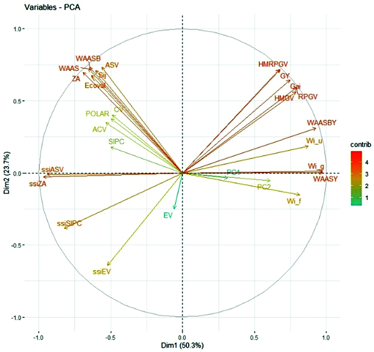
Figure 6: The rankings with genotypic grain yield and stability parameters are based on loading graphs obtained from principal component analysis

GY, grain yield; HMRPGV, Harmonic mean of the relative performance of the genotypic values; WAAS the weighted average of absolute scores; WAASB, weighted average of absolute scores for the best linear unbiased predictions (BLUPs) of the genotype-vs.-environment interaction; WAASY and WAASBY are the simultaneous selection indexes using WAAS and WAASB, respectively; ZA, the absolute value of the rela-tive contribution of the principal component axis of the interaction to the interaction; ASV, AMMI stability value; EV, averages of the squared eigenvector values; CV, coefficient of variation; ACV, adjusted coefficient of variation; POLAR, Power Law Residuals; Wi_g, Wi_f and Wi_u, Annichiarrico’s genotypic confidence index for all, favorable and unfavorable environments, respectively; Ecoval, Wricke’s ecovalence; Sij, Deviations from the joint-regression analysis; SIPC, sum of the absolute values of the IPCA scores; The ssi are the simultaneous selection indexes using AMMI-derived stability indexes; PC1 and PC2, the first and second principal component axis, respectively.

4  Discussion

In this study, we evaluated the performance of 12 agronomic traits of 28 different summer maize genotypes in two consecutive planting years (2018–2019) under the climatic conditions of Huang-huai-hai region. This region is the largest summer maize planting area in China. The performance of agronomic traits of germplasm resources is generally considered to be an important step in selecting genotypes suitable across different environments and with ideal agronomic traits, which can be used in future breeding programs to breed new and improved genotypes [33]. Genetic variability plays a vital role in improving the good progress for agronomic traits in plant breeding selection procedures. The results for the 12 evaluated agronomic traits showed that the genotype × environment interaction (GEI) was statistically significant (P < 0.001) based on the likelihood ratio test. This indicates that the genetic variation between genotypes varied across the environments. The magnitude of the GEI effect in the total variation is mainly attributed more to diversification than the genotypes [34]. In METs analysis, quantitative stability strategies are the basis for selecting genotypes, and are increasingly favored by agricultural researchers. The genotypes are evaluated based on the contribution of the scores of the first two principal component scores to the sum of square interactions, and the AMMI stability value (ASV) is used for this purpose [35–37]. It is possible to show how genotypic stability is quantified after introducing WAASB, which can be seen as a mixed model version of the ASV evaluation method. WAASB and ASV are consistent based on the first two IPCAs to evaluate genotype stability, and the ranking of both is highly consistent. It should be noted that for most of the analyzed traits, if there is a small proportion of GEI variance explained by the first two IPCAs in a certain trait, the ranking of genotypes based solely on ASV may be biased. WAASB will make up for this defect well, thus, the WAASB index will have a good effect on genotype evaluation in the future studies about quantifying genotypic stability [4,25,38]. WAASB × GY (or other agronomic traits) as one of the AMMI model biplots can be used to interpret the combination of trait observation values and stability, thereby evaluating the adaptability range of this genotype. Compared with the well-known AMMI1 biplot, the main advantage of the WAASB × GY biplot is that all IPCA axes are used, and GEI patterns that are not retained in IPCA1 can be considered in the genotypes ranking.

The MTSI evaluation system has unique and easy-to-understand characteristics. In addition, agricultural researchers have found that MTSI has many practical applications in breeding practices. For example, obtaining multiple agronomic traits and selection for mean performance and stability can be performed simultaneously [39]. The MGIDI index and the MTSI index also use the same rescaling process to select genotypes. This rescaling program places all the agronomic traits in the range of 0–100, which contributes to the definition of ideotype; thereby, all identical ideotype values for the evaluated agronomic traits are expressed as 100. This is only possible from the perspective of the selection direction required by the rescaling process. Future METs studies will have to rescale the evaluated traits by the breeders to define the value of the new maximum and minimum value of the agronomic trait after rescaling, respectively [21]. Based on the MGIDI index, selected genotypes were G22, G12, G10 and G1 as the promising maize genotypes. Apart from the genotypes selected above, G15, G4 and G26 were close to the cutting point, which means that this type of genotypes can show interesting features. Thus, genotypes near the cutting point need to obtain more attention from agricultural researchers. The genotypes G22 and G10 were selected by the MGIDI index and MTSI at the same time; it means that these two genotypes showed an ideal mean performance (MGIDI selection) and stability (MTSI selection). In this study, among different genotype ranking evaluation methods, MGIDI and FAI-BLUP, Smith-Hazel, MTSI had co-selected that the number of genotypes were 3, 1 and 2, respectively. Since there is a better consistency with other genotype ranking techniques, MGIDI will have more applications in future METs in terms of genotype rankings [40].

In previous studies, ranking ASV and mean performance of each agronomic trait were used to calculate a non-parametric simultaneous selection index (ssiASV) to identify genotypes with high performance and stability [41,42]. If the stability rating in such studies computed using ASV is reliable, simultaneous selection using ssiASV parameters will be promising. In view of the poor interpretation of the GEI model by the first two IPCAs, this ranking may be misleading. Therefore, in future fixed-effects model research, consider using simultaneous selection indexes based on important IPCA; these indexes include WAASY, ssiZA, ssiSIPC and ssiEV. WAASBY is considered to be a useful selection index when analyzing METs under the framework of the mixed effects model [43]. The reason why the WAASBY index results are more reliable than ssiASV is that all estimated IPCAs are considered after quantification of the stability, based on the mixed effect model and even the random effect model framework [4].

The main purpose of METs in summer maize genotypes is to identify and select excellent genotypes based on multiple agronomic traits and mega-environments. Taking into account the unpredictable environmental factors in GEI interaction research, different analysis models (PCA, Cluster analysis, AMMI and GGE) have been developed to clarify the effects of genotype, environment or their interaction [44]. The GYT biplot proposed in this study provides an analysis method for genotype evaluation based on multiple agronomic traits. This method is comprehensive and effective, as it ranks genotypes graphically based on the combined grain yield and the level of various evaluated agronomic traits, while showing the strengths and weaknesses of the tested genotypes. Because it does not involve subjective weights and cutting points, the analysis result of the GYT biplot is objective [23,45]. Among summer maize, high-yielding and stable maize genotypes are the first choice for farmers. However, grain yield is affected by a variety of agronomic traits. Thus, the GYT biplot provides maize breeders with an opportunity to evaluate genotypes and determine superior genotypes and superior indexes. The GYT method reveals the influencing factors by determining the high-efficiency performance of affected traits under a variety of environmental conditions. If the genotypes are evaluated based on the combination of traits and yield obtained from multiple locations, they will be very stable in all traits and yield across similar environments. For this reason, the GYT biplotting technique is used by some researchers to evaluate the performance of combining multiple traits with yield and multiple environments in breeding research [46,47]. Certain agronomic traits (GWE, ED, EL, and PH) directly increase the grain yield, while some agronomic traits directly reduce grain yield, such as LR, BTL and GP. In the current agricultural production, grain yield is not the only target. Those corn varieties that have both high grain yield and good agronomic traits are more favored by farmers. Therefore, when selecting the best genotypes, the influence of yield-traits combinations is more significant than the influence of individual traits.

5  Conclusion

In this study, 12 agronomic traits of 28 maize genotypes were evaluated across 24 different environments in a 2-year field experiment. In general, there was a statistically significant GEI effect for grain yield and the evaluated agronomic traits of maize genotypes in Huang-huai-hai region. This indicated that there may also be performance differences across the environments. In the multi-environment trials, the combination of AMMI model and BLUP technique made it possible to correctly describe GEI. We have used MGIDI, FAI-BLUP, Smith-Hazel and MTSI total of 4 evaluation methods of genotype ranking. In terms of total expected return, MGIDI was superior to the other three methods, which could be used as an ideal tool for genotype selection based on multiple traits. The GYT biplot technique provided information about the overall adaptability of the genotypes, and could clearly observe the stability and yield performance.

Acknowledgement: We thanks Professor Qiyi Tang for explaining us the AMMI model in this study.

Funding Statement: This research was funded by the Key Research & Development Projects of Hebei Province (20326305D), Key Research and Development Program of Hengshui City (2020014005C), Demonstration and Transformation of Major Achievements of Hebei Academy of Agriculture and Forestry Sciences in 2020, Innovative Project funded by Hebei Academy of Agriculture and Forestry Sciences, Special Fund for National System (Maize) of Modern Industrial Technology (CARS-02), the Science and Technology Support Program of Hebei Province (16226323D-X).

Conflicts of Interest: The authors declare that they have no conflicts of interest to report regarding the present study.

This work is licensed under a Creative Commons Attribution 4.0 International License, which permits unrestricted use, distribution, and reproduction in any medium, provided the original work is properly cited.