Journal of Renewable Materials

DOI: 10.32604/jrm.2021.014304

ARTICLE

Discrete Element Simulation of Asphalt Pavement Milling Process to Improve the Utilization of Milled Old Mixture

Jianmin Wu*, Bingbing Zhang, Chunsheng Wu, Zhiqiang Shu, Shaoqing Li and Jianqi Yang

Highway School, Chang’an University, Xi’an, 710000, China
*Corresponding Author: Jianmin Wu. Email: wujm@chd.edu.cn
Received: 16 September 2020; Accepted: 28 October 2020

1  Introduction

At present, construction stone resources are increasing scarce. It is urgent to save stone resources and improve the utilization of construction stones. However, due to the defects of the current milling process, the milling materials are prone to be broken, or there are many large agglomerates, resulting in a low recycling rate of milling materials. Due to the lack of reasonable milling parameters, the milling process causes a lot of unnecessary energy consumption, and the wear of the cutting tool is also increasing. In view of the above problems, if the discrete element virtual model of old asphalt pavement is established and the old pavement milling simulation is performed to optimize the milling parameters, the utilization rate of milling materials can be effectively improved, the milling energy consumption can be reduced, and the milling operation cost can be saved also.

At present, most of the finite element software is used to carry out the research of milling simulation of asphalt pavement, but the choice of discrete element method is relatively few. Among them, the analysis of the force of the cutting tool is a hot research topic, but there is a lack of research on the milling materials crushing, which is very important for the recycling rate of the milling materials. In terms of milling energy consumption, most researchers pay attention to the energy consumption of the milling machine during the milling process, but do not consider the energy consumption saved after the milling material utilization is increased. Xu [1] used ABAQUS to establish a practical pavement milling model, obtained a formula for calculating energy consumption of the milling machine, and analyzed the influence of milling parameters on milling operations. Guan [2] established a three-dimensional asphalt pavement milling model using discrete element method, quantified the force of the cutting tool in milling operations, and analyzed the influence of milling parameters on mechanical energy consumption and efficiency. Xiong [3] simulated the pavement milling process by finite element method, recorded the milling resistance and resistance moment of the cutting tool, and studied the influence of various parameters on the milling energy consumption coefficient. Zhao et al. [4] studied the force of the cutting tool when milling the elastic layer on the pavement, and used ADAMS (Automatic Dynamic Analysis of Mechanical Systems) software to simulate the milling of the pavement. The influence of the elastic layer with different parameters on the rotation angle of the cutting tool was analyzed. From the analysis of tool wear, Wu [5] believes that the main factors affecting the life of the cutting tool are the tool layout and installation angle. Based on the pavement milling finite element model, the milling effect of the cutting tool on the pavement under different milling speeds was analyzed, and the optimal milling speed was obtained. Van et al. [6] used DEM (Discrete Element Method) to simulate the rock milling process, and simulated different milling cutting tool. In each simulation, the cutting tool moves at a constant speed. The forces of the cutting tools in three orthogonal directions are recorded, and compared with the theoretical and experimental milling forces, it is pointed out that the milling depth is the main reason for tool wear. At present, there are few researches on energy consumption in the process of milling asphalt pavement. Scholars are keen to study the energy consumption during the construction and maintenance of the pavement. Shang et al. [7] studied the energy consumption and air emissions during the life cycle of roadbed and pavement. Kai et al. [8] established a discrete element thermal analysis model using discrete element method, and evaluated the heating effects of asphalt pavement during hot in-place recycling. Zhang et al. [9] established an energy consumption and emission model, and calculated the energy consumption and carbon emission composition of a typical semi-rigid base asphalt concrete pavement in China during the construction period. Wu et al. [10] studied the energy consumption calculation of the hot-in-place regeneration construction technology of asphalt pavement, and respectively measured the energy consumption of the raw material production, milling, transportation, paving and rolling during construction. Which provide a basis for the calculation of energy consumption in the pavement milling process.

The research on improving the recycling rate of milling materials in this paper is mainly to simulate the pavement milling by establishing a discrete element virtual model of the old asphalt pavement that meets the actual service life. In this study, aged SBS modified asphalt was used as a binder to prepare AC-16 asphalt mixture to simulate old asphalt pavement materials. PFC software was used to establish a microscopic model of the old asphalt pavement, and then the milling process of the old asphalt pavement was simulated. We analyzed the simulation results of milling, and the milling particles in contact can be regarded as larger clumps, which cannot be directly recycled and require secondary processing. Count the number of milling particles and contacts to quantify the number of large clumps and calculate the direct utilization rate of milling materials. Analyze the force of the cutting tool and the utilization rate of milling materials to determine the optimal milling speed and milling depth. The energy consumption of the milling process is measured according to the amount of milling materials, so as to quantitatively analyze the ratio of energy consumption reduction in the milling process after parameter optimization.

2  Materials and Methods

2.1 Asphalt Mixture Performance Test

Mostly, SBS modified asphalt mixture is used as the surface structure of highway asphalt pavements in China. And the milling of the pavement is mainly for the old asphalt pavement that has been in service for 10–12 years. According to the research results of Lu et al. [11,12], the rotating film oven aging test (RTFOT) can be used to simulate the long-term aging of SBS modified asphalt, and we can know the relationship between the aging time of asphalt and the service life of pavement. When the RTFOT aging time is 600 min, the service life of the road surface is about 11 to 12 years. Therefore, SBS modified asphalt with an aging time of 600 min was used as the bonding material to prepare the asphalt mixture specimens in this study, so as to simulate the old asphalt pavement with 11–12 years of service. By the way, in the long-term aging process of asphalt pavement, it is not only the aging of asphalt binder, but also the crushing of coarse aggregate under vehicle load. In fact, the aging of asphalt binder has a greater impact on the performance of the pavement so that we selected the main component of asphalt pavement aging, namely asphalt binder, as the object of this study.

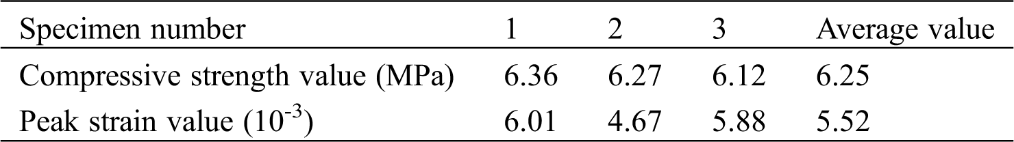
AC-16 asphalt mixture with 5% oil-stone ratio was prepared by using the aged SBS asphalt as the bonding material. SBS modified asphalt aged at 600 min is used in 100 mm × 100 mm AC-16 aged asphalt mixture standard sample. The uniaxial compression test was used to measure compressive strength and peak strain, and then compressive resilience modulus was calculated, which together serves as the basis for the internal parameter calibration of the asphalt mixture virtual model. See Tab. 1. You can refer to Standard Test Methods of Bitumen and Bituminous Mixtures for Highway Engineering (JTG E20-2011) [13] for specific test procedures.

Table 1: Compressive strength and peak strain

For testing the resilience modulus of the asphalt mixture, 6 test specimens were prepared. The resilience modulus of AC-16 asphalt mixture was calculated according to Eqs. (1) and (2). See Tab. 2.

—Strength under all levels of load, MPa; —Load applied to the test piece, N;

—Compressive resilient modulus, MPa; —Pressure at the 5th load, MPa;

—Test piece axis height, mm;

—The recoverable axial deformation after the origin correction corresponding to the fifth load, mm.

Table 2: Compressive resilience modulus

2.2 Establishment of Discrete Element Model for Asphalt Mixture

2.2.1 Calibration of Asphalt Mixture Model Parameters

The PFC built-in spherical particle generation method is used to model the virtual mixture of the asphalt mixture. According to the gradation median of each grade of AC-16 in the specification, the gradation of the AC-16 asphalt mixture virtual particle model with a 5% oil-stone ratio was determined (see Tab. 3). To save the calculation time, the fine aggregate, asphalt and mineral powder below 1.18 mm are uniformly replaced with particles with a diameter of 1.18 mm to simulate the asphalt mortar. So that generate a particle model of the initial state, as shown in Fig. 1a. The gradation particles are circulated through PFC until the particles in the model reach the final equilibrium state. See Fig. 1b.

Table 3: AC-16 asphalt mixture virtual particle model grading

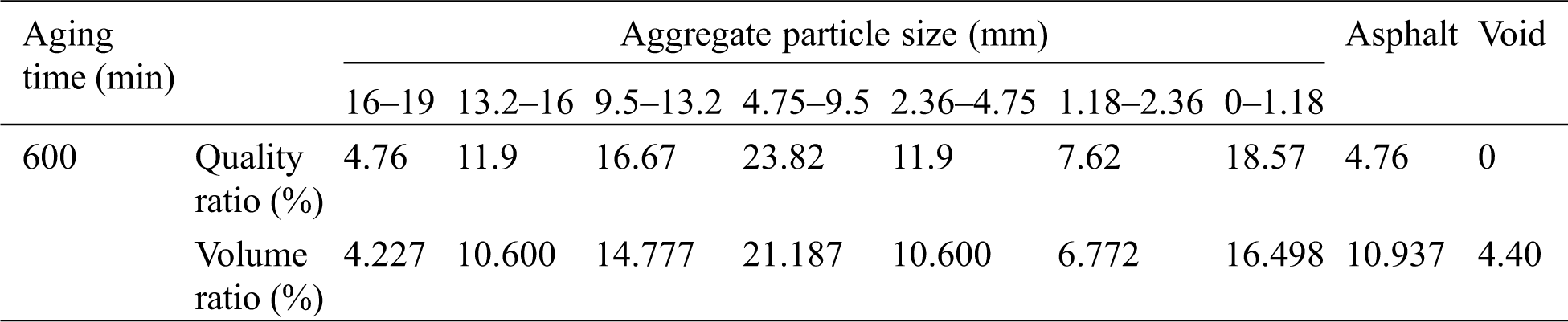
Figure 1: (a) State of the particle model, (b) Final state of the particle model, (c) Schematic diagram of uniaxial compression test

Referring to the indoor test requirements and process, in the establishment of the uniaxial compression virtual test, the rigid wall is selected as the boundary, and the upper and lower rigid plates are simulated by the upper and lower rigid walls. The upper and lower walls are respectively composed of two rigid triangular plates with boundaries, which keep the lower wall fixed and the upper wall was pressed at a constant speed. Through the FISH language programming, load evenly at 2 mm/min until the test piece is evenly damaged. The calculation stops when the stress load drops to 80% of the stress peak. The cylindrical virtual asphalt mixture test piece was placed between the two walls, as shown in Fig. 1c.

Generally, the contact interface of asphalt mixture is divided into at least three types: the interface between asphalt mortar and asphalt mortar, the interface between asphalt mortar and aggregates and the interface between aggregates and aggregates. In this paper, the parallel-bond contact type is used to characterize the contact between asphalt mortar and asphalt mortar, and the contact type between asphalt mortar and aggregates is the same as the above. The contact-bond contact type is used to characterize the contact between aggregates and aggregates. The results of the virtual uniaxial compression test were compared with the indoor uniaxial compression test, and after repeated checks, the parameters of the old asphalt pavement model were finally determined.

The parameter calibration process of the parallel-bond model is as follows:

(1) Effect and calibration of parallel-bond effective modulus

According to the relevant research experience [14,15], the research range of the parallel-bond effective modulus selected in this paper is 0.05 GPa–10 GPa. Combining the initial experimental calculations and the virtual test results, the parallel-bond model was selected to have a stiffness ratio of 0.5, a friction coefficient of 0.5, a normal tensile strength of 4.6 MPa, a cohesive force of 0.85 MPa, and an internal friction angle of 33°. Under these conditions, eight sets of parallel-bond effective modulus parameters were selected to study the effects on stress peak, peak strain and rebound modulus. The test results are shown in Tab. 4 below and Fig. 2.

Table 4: Effect of the parallel-bond effective modulus on test results

Figure 2: (a) Effect of the parallel-bond effective modulus on stress peak. (b) Effect of the parallel-bond effective modulus on peak strain. (c) Effect of the parallel-bond effective modulus on resilient modulus

It can be seen from Fig. 2a that when the parallel-bond effective modulus increases in the range of 0.05 GPa to 10 GPa, the stress peak of the uniaxial compression test gradually increases, the stress peak first increases sharply, then slowly increases, and finally the growth rate tends to gentle. According to Tab. 4, the difference between the minimum value and the maximum value of the stress peak is only 0.24 MPa. Therefore, the parallel-bond effective modulus has little effect on the stress peak and can be ignored. As can be seen from Fig. 2b, when the parallel-bond effective modulus is in the range of 0.05 GPa–0.5 GPa, the peak strain decreases sharply with the increase of the parallel-bond effective modulus; when the parallel-bond effective modulus is in the range of 0.5 GPa–10 GPa, The peak strain decreases slowly as the parallel-bond effective modulus increases and tend to be stable. Combined with the uniaxial compression failure characteristics and stress-strain curve of asphalt mixture, it is only necessary to study the influence of the model parameters on stress peak and resilient modulus to reflect the mechanical response of asphalt mixture under uniaxial compression test. Therefore, peak strain is no longer considered in other parameter calibration studies.

According to Fig. 2c, the influence of the parallel-bond effective modulus on the resilient modulus was further analyzed. When the parallel-bond effective modulus increases in the range of 0.05 GPa–10 GPa, the resilience modulus linearly increases with the parallel-bond effective modulus. According to this rule, multiple sets of data are used to fit a linear equation to obtain a rough parallel bond effective modulus. Then keep adjusting the parallel-bond effective modulus until the resilience modulus obtained by the simulation is consistent with the indoor test results of the asphalt mixture. In this study, the linear correlation R2 of the fitted line is 0.966, which greatly facilitates the calibration of the model parameters. According to the indoor test, the compressive strength is 6.12 MPa and the resilience modulus value is 1.046 GPa, and the parallel-bond effective modulus can be initially determined to be in the range of 0.1 GPa–0.5 GPa.

(2) Effect and calibration of parallel-bond stiffness ratio

In PFC, the parallel-bond stiffness ratio is the ratio of the normal stiffness to the tangential stiffness at the bond between the particles. Shi et al. [16] researches show that the parallel-bond stiffness ratio affects the longitudinal strain and transverse strain of the virtual specimen. According to Chehreghani et al. [14] and Xia et al. [17] research results on micro parameters in the parallel-bond model, in this section, the model was selected to have a parallel-bond effective modulus of 0.5 GPa, a friction coefficient of 0.5, a normal tensile strength of 4.6 MPa, a cohesive force of 0.85 MPa, and an internal friction angle of 33°. Under these conditions, the effects of seven sets of parallel-bond stiffness ratios between 0.25 and 3.0 on the virtual test results were analyzed. The test results are shown in Tab. 5 and Fig. 3.

Table 5: Effect of parallel-bond stiffness ratio on test results

Figure 3: (a) Effect of parallel-bond stiffness ratio on stress peak. (b) Effect of parallel-bond stiffness ratio on resilient modulus

It can be seen from Fig. 3a that the stress peak increases first and then decreases as the parallel-bond stiffness ratio increases. According to Tab. 5, the parallel-bond stiffness ratio is in the range of 0.25–3.0, and the corresponding stress peaks are between 3.71 MPa and 3.78 MPa, and the difference is only 0.07 MPa. Therefore, the parallel bond stiffness ratio has less influence on the stress peak. It can be seen from Fig. 3b and Tab. 5 that as the increase of the parallel-bond stiffness ratio, the resilient modulus first increases, and the back change has no obvious trend. The difference between the maximum value and the minimum value is 0.052 GPa, so that the effect of parallel-bond stiffness ratio on resilient modulus could be ignored. In summary, the parallel-bond stiffness ratio has no significant effect on the test results. According to the relevant research experience [18,19] and the above research on the parallel bond stiffness ratio, the value of the parallel-bond stiffness ratio is initially determined to be 0.5–2.0.

(3) The calibration process of bond strength and friction coefficient is similar to the calibration process of the parallel-bond effective modulus. Finally, it is determined that the parallel-bond normal strength is between 6.9 and 9.2 MPa, and the value of the friction coefficient is between 1.0 and 2.0.

The parameter calibration process of the contact-bond model is as follows:

In the asphalt mixture model, almost all of the aggregates is covered by mortar, only a small part of the aggregates is in direct contact with the aggregates, and the number of contacts between the aggregates is very small, accounting for less than 5% of the total number of contacts. Therefore, there is no need to set up a separate test to calibrate the contact-bond parameters between the aggregates and the aggregates, and the same calibration method as above can be used.

2.2.2 Determination of Microscopic Parameters of Asphalt Mixture

The specific virtual model parameters need to be adjusted in combination with the indoor test. By continuously adjusting the model parameters until the virtual test results are basically consistent with the indoor test values. The error between the virtual uniaxial compression test result and the actual measurement result is small, as shown in Tab. 6. The parallel-bond contact parameters between asphalt mortar and asphalt mortar are as follows: The parallel-bond effective modulus is 0.21 GPa, the stiffness ratio is 0.5, the normal strength is 7.24 MPa, and the friction coefficient is 1.0. The parallel-bond contact parameters between asphalt mortar and aggregates are the same as the above. The contact-bond contact between aggregates and aggregates are as follows: the contact-bond effective modulus is 0.55 GPa, the stiffness ratio is 1.0, the normal strength is 1.07 MPa, and the friction coefficient is 1.0. Based on the calibrated model parameters, a discrete element model of asphalt mixture is established to prepare for pavement milling simulation.

Table 6: Error between simulation results and actual measurement results

At present, the discrete element model of the old asphalt pavement has been established, and the material is ready for the subsequent milling simulation. In this paper, the results of road milling simulation were analyzed from two perspectives: the force of the milling cutting tool and the utilization rate of the milling materials. We use a single variable method to study the influence of milling speed and milling depth on the force of the cutting tool and the utilization rate of milling materials. Therefore, the optimal milling speed and milling depth were determined.

3  Results and Discussions

3.1 Establishment of Asphalt Pavement Milling Model

During the asphalt pavement milling process, it is the cutting tools on the milling drum to damage the pavement mainly. The cutting tools displacement on the milling drum is spirally symmetrical in milling machine. In order to reduce resistance during cutting, generally, only one tool is set on the same rotating plane except edge tool and vertical tool is set in the same rotary plane. So, in this study, only one tool is used to simulate the milling process of the old asphalt pavement. In this paper, when using PRO/ENGINEER for tool 3D modeling, in order to achieve a more accurate simulation of the asphalt pavement milling process, a 3D model including the components of the tool was established, as shown in Fig. 4a. Save the 3D model built by PRO/E in STL format and import it into PFC3D software. The 3D model of the tool in PFC is shown in Fig. 4b below.

Figure 4: Cutting tool model. (a) Before import (b) After import

In this paper, a cuboid with dimensions of 100 mm in length, 80 mm in height, and 50 mm in width was selected in PFC to establish the old asphalt pavement model. The old asphalt pavement model is generated in this space according to the asphalt mixture model established above, as shown in Fig. 5a below. The simulation model of the old asphalt pavement after replacing the coarse aggregate sphere particles with the breakable cluster unit is shown in Fig. 5b.

Figure 5: (a) Preliminary generated pavement simulation model. (b) Pavement simulation model after cluster replacement. (c) Milling simulation model of old asphalt pavement

The PFC3D asphalt mixture model is fixed, and a milling cutter head is arranged on the left side. The rigidity of the cutting tool is set to be much greater than the rigidity of asphalt mixture model to simulate the hardness of the actual milling cutting tool. And the milling parameters of the cutting tool are set through the fish language in PFC to simulate the actual milling process of the old asphalt pavement. The old pavement milling model is shown in Fig. 5c, where α is the cutting angle of the cutting tool and H is the milling depth of the cutting tool.

3.2 Simulation of Asphalt Pavement Milling Process

In the process of milling simulation on the old asphalt pavement, the force change of the cutting tool and the utilization rate of the milling material were studied. There are three main influencing factors, namely cutting angle, milling speed and milling depth. According to the research experience of many experts [20−22], when the cutting angle is 42°, the service life of the cutting tool is high and the work is stable. Therefore, the cutting angle of the cutting tool selected here is 42°.

According to relevant research experience [23−25], the milling speed is generally controlled between 0.1 m/s–2.5 m/s. However, in practice, too high or too low milling speed is detrimental to the service life of the cutting tool, and the milling materials is not ideal. Therefore, the milling speeds used in this paper are 0.5 m/s, 1 m/s, and 1.5 m/s. The milling machine is mainly used for milling the upper layer or upper middle layer of asphalt pavement, and its thickness is generally within 50 mm [26,27]. Therefore, the milling depths of 20 mm, 30 mm, 40 mm, and 50 mm are used in this paper to study and analyze the impact on the cutting tool force.

3.2.1 Determination of Milling Speed Parameters

Cutting depth and angle are fixed to investigate the effect of milling speed on the force of the cutting tool and analyze the corresponding milling materials utilization. Cutting depth is set to 40 mm, cutting angle is 42°, and cutting speeds are 0.5, 1.0, and 1.5 m/s. The milling processes at different cutting speeds are shown in Fig. 6. The amount of milling materials and the contacts were recorded (as shown in Tab. 7), which reflected the effect of pavement milling to some extent.

Figure 6: Cutting diagram at different milling speeds. (a), (b), and (c) refer to the cutting diagram at cutting speeds of 0.5, 1.0, and 1.5 m/s, respectively

Table 7: Number of milling materials and the contacts at each milling speed

As can be seen from Fig. 6 and Tab. 7 above, during the simulation of old road milling at these three milling speeds, more fines were milled and less bulky materials were milled. When the cut-in angle and the milling depth are constant, as the milling speed increases, the number of milling materials and the contacts gradually increase.

Analysis from the influence of milling speed on cutting tool force.

In order to better analyze the effect of cutting speed on cutting tool force, in this paper, the force value data recorded in each direction after the milling simulation is output as a CSV format file. Originpro data processing software is used to draw the force change diagram of the cutting tool in all directions, as shown in Fig. 7 below.

Figure 7: Force diagram of cutting tool at different milling speed. (a), (b), and (c) refer to the force diagram of the cutting tool in the X-, Y-, and Z-directions, respectively, at different milling speeds

Fig. 7 shows that the cutting tool moves in the positive direction of X and receives the force in the negative direction of X. The force of the cutting tool at each speed appears to increase first and then stabilize. And as the milling speed of the cutting tool increases, the milling resistance that the cutting tool receives in the X-direction increases significantly. The force in the Y-axis direction oscillates up and down around 0 N, which is consistent with no displacement of the cutting tool in the Y-axis direction during milling simulation. The tool is subjected to a force in the negative direction of the Z-axis. At each speed, the force value of the cutting tool gradually increases and then decreases, and finally the force value shows an oscillating trend with a large amplitude. It can be seen that the cutting tool force in the same direction at different milling speeds is very different. This is because the path of the milling cutting tool at the three milling speeds is different, and the cohesion between particles in contact with the cutter head is not the same. In order to better analyze the influence of effect of cutting speed on cutting tool force, in this paper, the cutting tool force data value at a cutting angle of 42° and a milling depth of 40 mm is extracted from the PFC3D. The average force of the cutting tool in each direction at each milling speed is calculated, as shown in Tab. 8 below.

Table 8: Mean force of the cutting tool in different directions (N)

From Tab. 8 above, as the milling cutter’s milling speed increases, the combined force of the tool in three directions gradually increases, and the cutting tool force in X-direction gradually increases, and the force in the Y and Z-directions increases first and then decreases. Of the three directions, the average force of the cutting tool in the X-direction is the largest, the force value is in the range of 160 N–380 N. The average force of the Z-direction is in the range of 130 N–210 N, and the average value of the force in the Y direction is the smallest, just 26.8 N. It can be seen that the milling speed has the most significant effect on the forces in the X and Z-directions of the cutting tool. The forces in the X and Z-directions are the main factors of the combined forces on the cutting tool. The effect of the Y-direction on the force of the cutting tool could be negligible.

Comparing the force on the cutting tool at the three milling speeds, the combined force on the tool is the smallest at a milling speed of 0.5 m/s, that is, the tool wears the least, which can enhance the durability of the tool and improve economic benefits.

Analysis from the direct utilization rate of milling materials:

According to the milling simulation results, the number of milling materials (Nij) and the number of milling materials contacting (nij) can be counted. Among them, i is the milling speed, taking 1, 2 and 3 to represent 0.5, 1.0 and 1.5 m/s respectively; j is the milling depth, taking 1, 2, 3 and 4 to represent 20, 30, 40 and 50 mm respectively. From the analysis of the milling effect, the larger agglomerate is formed by the aggregation of two or three particles. Since two particles aggregate to produce one contact, and three particles aggregate to produce two or three contacts, the average value can be taken for the convenience of calculation, so each contact can be considered to correspond to 1.5 particles. Milling materials that are not in contact are considered to be directly recyclable and do not require secondary processing. According to relevant research experience [28], the following formula can be used to calculate the direct utilization rate of milling material (Rij):

The corresponding milling material utilization rate can be calculated combining the data in Tab. 7.

The calculation results show that: under the condition of a milling depth of 40 mm, the milling material utilization rates corresponding to the three milling speeds are 67.9%, 69.0%, and 65.9%, respectively. There is little difference between the three. In this case, it can be considered that the milling speed has no significant effect on the utilization of milling materials. Comparing the force on the cutting tool at the three milling speeds, the combined force on the tool is the smallest at a milling speed of 0.5 m/s, that is, the tool wears the least. In summary, for AC-16 asphalt mixtures with actual service life of 11–12 years, the optimal milling speed of the cutting tool is 0.5 m/s.

3.2.2 Determination of Milling Depth Parameters

After fixing the cutting speed and angle, the milling force of the tool with different milling depths is calculated. The simulation conditions are as follows: milling speed of 0.5 m/s; cutting angle of 42°; and milling depths of 20 mm, 30 mm, 40 mm, and 50 mm. The milling processes at different milling depths are shown in Fig. 8. The amount of milling materials and the contacts were recorded, as shown in Tab. 9.

Figure 8: Cutting diagram with different cutting depths. (a), (b), (c), and (d) refer to the cutting diagram with cutting depths of 20, 25, 30, and 40 mm, respectively

Table 9: Number of milling materials and the contacts at each milling depth

As can be seen from Fig. 8 and Tab. 9, when the cutting angle and the milling speed are fixed, as the milling depth increases, the number of milled materials and the contacts gradually increases.

Analysis from the influence of milling speed on cutting tool force.

The force in each direction of the cutting tool was plotted into a figure, as shown Fig. 9.

Figure 9: Force diagram of cutting tool with different cutting depths. (a), (b), and (c) refer to the force diagram of the cutting tool in the X-, Y- and Z-directions with different cutting depths, respectively

Fig. 9a shows that the cutting tool is subjected to the negative force of the X axis when moving in the positive X-direction. With the increase of the milling depth, the cutting tool force in the X-direction increases at each milling depth, and then varies. The cutting tool force gradually increases at each depth within a displacement of 0 mm to 20 mm in the X-directioni. When the cutter head is displaced by 20 mm and 30 mm in the X-direction, the cutting tool force in X-direction is reduced to oscillate up and down by 200 N, When the displacement is 50 mm in the X-direction, the cutting tool force in X-direction is increased to oscillate up and down by 400 N. The milling effect of the cutting tool has reached a stable period, but the force change trend of the tool at each depth is different. This difference is caused by the different milling path of the tool at each depth. Fig. 9b shows that the cutting tool force in the Y-direction at each milling depth oscillates up and down around 0 N, but the changes are not consistent. And the peak stress of the cutting tool in the Y-direction at each milling depth does not exceed 80 N, which is consistent with the cutting tool in the Y-direction without displacement during milling simulation. Fig. 9c shows that the cutting tool force in the Z-direction is negative along the negative direction of the Z-axis, which is consistent with the movement of the cutting tool in the positive direction of the Z-axis. With the increase of the milling depth, the cutting tool force in the Z-direction increases at each milling depth, and then varies. The scatter plots of the cutting tool force values at various milling depths in the 0 mm to 10 mm displacement in the X-direction overlap more, but they gradually increase. It can be seen that the cutting tool force in the same direction at different milling depths is very different. On the one hand, this is caused by the different milling paths of the cutting tool. On the other hand, as the milling thickness increases, the internal resistance of the mixture is more complicated. Therefore, the force state of the cutting tool has undergone complex changes.

The average force of the cutting tool in each direction at each milling depth is calculated, as shown in Tab. 10 below.

Table 10: Mean force of the cutting tool in different directions (N)

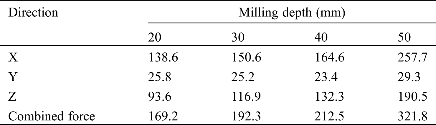
Tab. 10 shows that with the increase of the milling depth, the combined force of the cutting tool in three directions gradually increases. In the milling depth of 20 mm–40 mm, the combined force increase is relatively gentle, and the difference is small. The combined force at 50 mm milling depth suddenly increased to 321.8 N, mainly due to the apparent increase in the average force in the X-direction. At each depth, the mean value of the cutting tool force in the X and Z-directions is greater than the force in the Y-direction. The force value in the X, Y, and Z-direction is in the range of 130 N–260 N, 90 N–200 N, and 20 N–30 N. It can be seen that the milling depth has the most significant influence on the forces in the X and Z-directions of the cutter head. And, the forces in the X and Z-directions of the cutting tool have the greatest effect on the combined force of the tool, and the forces in the Y-direction of the cutting tool have a very small effect on the combined force, which can be ignored.

Analysis from the direct utilization rate of milling materials:

According to Eq. (3) and the data in Tab. 9, the milling material utilization rate corresponding to different milling depths is calculated under the condition of milling speed of 0.5 m/s, and the results are as follows:

Among them: R11 = 85.3%, the highest value, is obviously better than R12 = 76.2%, R13 = 67.9%, R14 = 65.3%. Therefore, from the perspective of milling material utilization, when the milling depth is 20 mm, the direct utilization of milling materials is the highest. In summary, comparing the force on the cutting tool at the four milling depths, the combined force on the tool is the smallest at a milling depth of 20 mm, that is, the tool wears the least, which can enhance the durability of the tool and improve economic benefits. In addition, the utilization rate of milling materials is the highest, with a value of 85.3%.

Finally, the optimal milling parameters were determined, that is, the optimal milling speed is 0.5 m/s and the optimal milling depth is 20 mm. In this case, the direct utilization rate of milling materials is the highest, and its value is 85.3%. Under general milling conditions, that is, the milling speed is 0.5 m/s, the milling depth is 40 mm, and the direct utilization rate of milling materials is 67.9%. Therefore, it can be known from the results of this study: After parameter optimization, the utilization rate of milling materials can be increased by 17.4%.

3.3 Energy Consumption Calculation in the Pavement Milling Process

The energy consumption during the construction of asphalt pavement can be divided into the following parts: raw material production, milling, mixture production, transportation, paving and rolling, etc. In this paper, we mainly calculate the energy consumption of raw material production, milling process and transportation process. Common milling parameters are represented by a milling speed of 0.5 m/s and a milling depth of 40 mm [21], which can be used as a control group for comparison with the optimal milling parameters. Since most of the milling material is uniform in thickness and there are few large particles, the volume of the milling materials can be measured by the quantity of the milling materials. And the density of the milling materials is very close, so its mass can be approximated by the quantity of milling materials. That is to say, the quantity of milling materials is proportional to its mass [29]. The relationship can be simplified as follows:

Among them: Mij (unit: t) is the mass of milling materials corresponding to Nij; Nij (already introduced in 3.2.1) is the total quantity of milling material (unit: pieces); k is a constant (unit: t/piece). The energy consumption of the milling process and the transportation process can be directly obtained by calculating the amount of milling materials, but the energy consumption calculation of the raw materials production also needs to rely on the utilization rate of the milling materials. The higher utilization rate of milling materials, the less waste of milling material, the more stone materials are saved, and the more energy is saved. The wasted milling materials need prepare new crushed stone as a supplement. Therefore, the mass of crushed stone can be calculated by the utilization rate of milling materials, and then the energy consumption required by the preparation process can be calculated.

According to the calculation and analysis process of Cui [30] on the energy consumption of hot recycled asphalt pavement, it can be concluded that the energy consumption for manufacturing crushed stone is 31.99 MJ • t-1, the energy consumption for milling and planing is 49.36 MJ • t-1, and the energy consumption for transportation is 67.10 MJ • t-1. The number of milling materials in the control group(N13) is 397, and the utilization rate of milling materials is 67.9%. The number of milling materials in the optimal group (N11) is 276, and the utilization rate of milling materials is 85.3%. Through calculation, the total mass of milling materials are: M13 = 397k•t, M11 = 276k•t. The mass of unused milling materials, that is, the mass of crushed stone required are: m13 = M13 × (1 − R13) = 397 × (1 − 0.679) = 127.4 k•t, m11 = M11 × (1 − R11) = 276 × (1 − 0.853) = 40.6 k•t.

Therefore, when the milling speed is 0.5 m/s and the milling depth is 40 mm (i = 1, j = 3).

The energy consumed to make gravel is: m13 × 31.99 MJ•t-1 = 127.4 k•t × 31.99 MJ•t-1 = 4075.53k (MJ). The energy consumed in the milling process is: M13 × 49.36 MJ•t-1 = 397k•t × 49.36 MJ•t-1 = 19595.92k (MJ). Energy consumption during transportation process: M13 × 67.10 MJ•t-1 = 397k•t × 67.10 MJ•t-1 = 26638.70k (MJ). The total energy consumed is EA = 4075.53k (MJ) + 19595.92k (MJ) + 26638.70k (MJ) = 50310.15k (MJ).

When the milling speed is 0.5 m/s and the milling depth is 20 mm (i = 1, j = 1).

The energy consumed to make gravel is: m11 × 31.99 MJ•t-1 = 40.6 k•t × 31.99 MJ•t-1 = 1298.79k (MJ). The energy consumed in the milling process is: M11 × 49.36 MJ•t-1 = 276k•t × 49.36 MJ•t-1 = 13623.36k (MJ). Energy consumption during transportation process: M11 × 67.10 MJ•t-1 = 276k•t × 67.10 MJ•t-1 = 18519.60k (MJ). The total energy consumed is EB = 1298.79k (MJ) + 13623.36k (MJ) + 18519.60k (MJ) = 33441.75k (MJ).

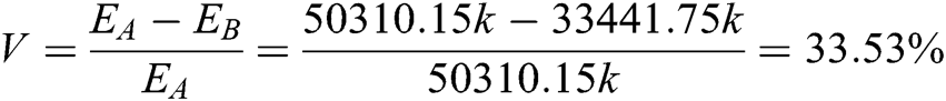
The ratio of energy consumption reduction by using the optimal milling parameters relative to the common milling parameters is V:

4  Conclusion

In this paper, the discrete element software PFC was used to simulate the milling process of the old asphalt pavement. In the process, the force of the cutting tool and the utilization rate of milling materials were analyzed to determine the optimal milling parameters. The specific conclusions are as follows:

(1)   The milling speed has the most significant effect on the forces in the X and Z directions of the cutting tool. When the milling speed is 0.5 m/s, the combined force of the cutting tool is the smallest, which is beneficial to reduce the tool wear. In this case, when milling old asphalt pavement, the optimal milling speed of the cutting tool is 0.5 m/s.

(2)   As the milling depth increases, the combined force of the cutting tool in three directions gradually increases. When the milling depth is 20 mm, the combined force of the cutting tool is the smallest, which is beneficial to reduce the tool wear. In addition, the utilization rate of milling materials is the highest. In this case, when milling old asphalt pavement, the optimal milling depth of the cutting tool is 20 mm.

(3)   For the old asphalt pavement with a service life of 11–12 years, at a cutting angle of 42°, when the milling speed of the cutting tool is 0.5 m/s and the milling depth is 20 mm, the cutting tool wears less, and the direct utilization rate of the milling materials is the highest, the value is 85.3%. After parameter optimization, the utilization rate of milling materials can be increased by 17.4%.

(4)   The ratio of energy consumption reduction by using the optimal milling parameters relative to the common milling parameters is 33.53%, which has significant energy saving benefits and reduces the cost of milling operations.

Acknowledgement: We thank Mr. Liu Yu from Chang’an University for his suggestions on pavement milling simulation analysis. We thank all the participants in this study.

Funding Statement: The authors received no specific funding for this study.

Conflicts of Interest: The authors declare that they have no conflicts of interest to report regarding the present study.

This work is licensed under a Creative Commons Attribution 4.0 International License, which permits unrestricted use, distribution, and reproduction in any medium, provided the original work is properly cited.