Effects of T-Factor on Quantum Annealing Algorithms for Integer Factoring Problem

1  Introduction

The hardness assumption of the integer factorization problem (IFP) [1] is one of the most important cryptographic primitives for modern information security. Based thereon, the well-known RSA cryptosystem [2] as well as its variants [3] are assumed to still be secure and widely used today. In fact, our confidence in this comes from the classical computational complexity for solving IFP. To factor a larger integer N, the current fastest classical algorithm is the number field sieve (NFS) method that has sub-exponential complexity with respect to the bit-length of N, expressed by O(e(64/9∖log N)1/3 log (log N)2/3). According to this formula, an IFP-based cryptosystem with 1024-bit modulus has merely 80-bit security strength. At CRYPTO 2020, a 795-bit number was factored [4], and the previous records were the factorization of RSA-768 in 2009 [5]. Today, to meet a 128-bit security strength for IFP based crytosystems, the suggested modulus bit-length is approximately 3072 [4].

Even so, our confidence is losing due to the quick development of quantum computation. Theoretically, Shor’s quantum algorithm can factor N within polynomial-time complexity. More precisely, to factor N, we need only O((log N)3) quantum operators and O(log N) qubits by using Shor’s algorithm. But in practice, this theoretical quantum computation complexity is challenged by at least two gaps: One is how to implement quantum gates with (nearly) 100% fidelity, and the other is how to implement sufficient (say 3072) logical qubits. According to the reported IBM scaling quantum technology, a quantum system with 1 million (physical) qubits could be built in the near future [6]. However, the estimated quantum error correction bits that Shor algorithm will use can reach the order of one million and even one billion [7]. This makes Shor’s algorithm require a lot of quantum computing resources when factoring large integers. In the NISQ era Shor algorithm have been shown can only factor integer N≤100, i.e., less than 7 bits, in recently reported experiments [8].

Interestingly, the methods of solving IFP by using quantum computers have new developments besides Shor’s algorithm. In 2001, Farhi et al. [9] introduced the quantum adiabatic theorem for the first time, and realized the factorization of N=143. In 2018, Jiang et al. [10] used the D-Wave [11] 2000Q platform to improve the multiplication table of the annealing algorithm and successfully factored the number N=376,289 by using 94 logical qubits. Shortly afterward, Peng et al. [12] further advanced Jiang’s work by reducing the number of qubits used according to the constraints on the integers to be factored and the number of carrying numbers involved in the multiplication table. In 2020, Wang et al. [13] used a new independent model with 88 qubits to successfully factor N=1,028,171. The D-Wave platform uses qubits as logical nodes on the Chimera graph [14], rather than gate units in the quantum circuits on which Shor’s algorithm relies. In 2022, Saida et al. [15] also successfully implemented the quantum annealing factorization of the multiplier Hamiltonian using superconducting flux qubits. The performance of quantum annealing algorithm in NISQ (Noisy Intermediate-Scale Quantum) [16,17] era is quite remarkable. Most recently, it is reported that a 48-bit integer was factored by using a classical-quantum hybrid method: Classical Schnorr lattice integer factoring method, plus a superconducting quantum optimization using only 10 qubits [18].

In this work, we would like to report an interesting observation regarding the performance of quantum annealing algorithm (QAA for short) for integer factorization. In the above-mentioned experiments, improvements on the multiplication table are employed to reduce the required qubits. However, in our experiments based on D-Wave platform, we found that the multiplier filling degree (named T-factor) in the QAA algorithm has an observable effect on the performance of the annealing algorithm. In the classical algorithm, the larger the difference between the two multipliers is, the easier the integer is to factorize. However, in the quantum annealing factorization experiment, we conclude that the bigger the difference between the bit-lengths of the two multipliers p and q, the harder for QAA to factor N=pq. Finally, we try to present our explanation of this observation based on the advantage of quantum tunneling effect in potential energy field.

The structure of this paper is as follows. In Section 2, the background required for this article is presented. The integer factorization and simulated annealing algorithm are briefly introduced, and the advantage of QAA is introduced. In Section 3, the evaluation criteria of algorithm performance are first determined. After the traversal annealing experiment, the processed data are also presented. In Section 4, we propose the concept of T-factor and explain why T-factor affects algorithm performance. In Section 5, through the experimental data, we summarize the indicative role of T-factor in actual integer factorization, the deficiency of T-factor is also discussed.

2  Preliminaries

2.1 Classical Simulated Annealing

The idea of simulated annealing was introduced into combinatorial optimization algorithm by Kirkpatrick et al. [19] in 1983, it is a stochastic optimization algorithm based on Monte-Carlo iterative solving strategy. The actual operation flow of simulated annealing algorithm is as follows.

Set the initial temperature T0, and randomly generate the initial solution $x_0$, and calculate the corresponding objective function value E(x0). Then, let T=λT, λ∈(0,1) is the decreasing rate of temperature. A random perturbation is applied to the current xt to produce a new solution xt+1 in the neighborhood. The corresponding function value of xt+1 is E(xt+1). Calculate ΔE=E(xt+1)−E(xt). Judge whether to accept the new solution according to the Metropolis criterion. If ΔE<0, accept the current solution; otherwise, judge whether to accept according to probability. The process of perturbation and generation of new solutions is repeated as far as the temperature allows, and finally the algorithm stops when the temperature reaches the termination level.

2.2 Quantum Annealing and D-Wave

Quantum annealing is a generic name of quantum algorithms that use quantum-mechanical fluctuations to search for the solution to an optimization problem [20]. The traditional simulated annealing algorithm uses thermodynamics to make the system cross the potential barrier. Quantum annealing algorithm uses quantum tunneling effect to achieve this goal. As in the traditional simulated annealing algorithm with slow cooling, we first set the quantum fluctuation strength to a large value to find the global structure of the solution space. After that we gradually reduce the strength of the fluctuations, hoping to recover the original system in the lowest energy state. Quantum annealing algorithm is a general algorithm, which can be applied to any combinatorial optimization problem.

The evolution of quantum system can be described by the time-varying Schrodinger equation [21]

ih2π∂∂t|Ψ(t)>=H(t)|Ψ(t)>(1)

and

H(t)=Hcl+Hkin(t)(2)

Hcl is the potential energy term, and Hkin(t) is the kinetic energy term suitable for the system. When optimization starts, H(t) has a large initial value, and then it shrinks gradually until it gets down to zero [22]. For the integer factorization problem, we will target function F=(N−pq)2 mapping to the Hamiltonian of quantum annealing can be, when we find the Hamiltonian of the ground state energy, namely to find the zero solution of the optimization function.

In the D-Wave quantum annealing platform, the gates in the multiplier are converted into a mapping of qubits and couplers. As shown in Fig. 1, the full adder is converted to a yellow pentagonal star, the half adder to a blue square, and the AND gate to a pink triangle. When we fix the output to the integer we need to factorize, the energy ground state of the entire quantum circuit system is determined. The potential energy Hcl of the system is the difference between the current state and the goal state, and the kinetic energy Hkin(t) of the system is the current “temperature” provided by the annealing algorithm.

Figure 1: (a) Shows the transformation of AND gate into quantum circuit state; (b) is the circuit diagram of the classical multiplier; (c) shows the transformation of gate circuit into quantum circuit; (d) shows the quantum circuit diagram after the conversion is completed (Image from the official D-Wave website)

Quantum tunneling effect: In quantum mechanics, we have

ΔEΔt≈h¯2(3)

where ΔE and Δt are the uncertainties of energy and time [23], respectively, and h¯ is the reduced Planck constant. If the uncertainty of time is assumed to be Δt, then ΔE=h¯2Δt. After the particle gets the extra energy ΔE, if there is E+ΔE>V, the particle can go directly over the barrier to the other region. As shown in Fig. 2, when the annealing algorithm is carried out to the end, a potential energy barrier will be generated between the local and global optimal solutions. The quantum tunneling effect can ignore this barrier, which makes it easier to obtain the global optimal solution.

Figure 2: Compared with the conventional simulated annealing algorithm, the quantum annealing algorithm can use the quantum tunneling effect directly to ignore the potential energy barriers to the optimal solution

3  Research Methods of Quantum Annealing

3.1 Hamiltonian Modeling of the Integer Factorization Problem

We use the quantum annealed integer factorization algorithm provided by D-Wave platform to carry out experiments. The objective function is

F=(N−pq)2(4)

set l1=⌊log2⁡(p)⌋+1, l2=⌊log2⁡(q)⌋+1, respectively. Since any prime number greater than 2 is odd, we can express it as: p=(xl1xl1−1 …x11)2 and q=(xl2xl2−1 …x11)2. The processed integers and the objective function are put into a constrained bivariate quadratic model, so that the energy of the whole objective function is mapped into a Hamiltonian.

First, the time-varying Hamiltonian of a quantum system is

H(t)=(1−tT)HB+tTHP(5)

where the duration T defines the time scale over which the function runs and controls the rate of change of the Hamiltonian over time. HB is the initial Hamiltonian, which defines the x-basis of the i-th qubit using the Pauli operator.

HB=−∑σx(i)(6)

HP is the final Hamiltonian, where the Pauli operator σz(i) defines the z-basis of the i-th qubit, and the local domain hi and the coupling Jij together define the problem instance.

HP=−∑hiσz(i)+∑Jijσz(i)σz(j)(7)

The Ising model [24] is thus established.

Here we further refine the Ising model as shown in Eq. (8). As shown in Fig. 1d, we connect the integer to be decomposed and the set multiplier into the optimized quantum circuit after conversion. The qubits form the local domain hi, the coupling between the qubits is Jij, and we are looking for the lowest energy state of this quantum system as a whole.

Hising=−A(s)2(∑i⁡σ^x(i))+B(s)2(∑i⁡hiσ^z(i)+∑i > j⁡Ji,jσ^z(i)σ^z(j))(8)

•   A(s) represents the transverse or tunneling energy. It is equal to δq, the energy difference between two eigenstates of an rf-SQUID qubit [25] with no externally applied flux.

•   B(s) is the energy of the applied and problem Hamiltonian. It is equal to 2MAFMIp(s)2, where MAFM denotes the maximum achievable available mutual inductance between flux qubit pairs, and Ip is the magnitude of the current flowing in the body of the rf-SQUID loop.

3.2 Relationship between Annealing Times and Algorithm Execution Time

The integer factorization procedure of the D-Wave quantum annealing platform allows us to set different numbers of inner loops in the code, which we collectively refer to here as the number of annealing runs. In the annealing algorithm, the number of annealing runs has a linear relationship with the time that the program runs, as shown in Fig. 3.

Figure 3: There is a linear relationship between annealing time and number of annealing runs we can artificially limit the number of annealing runs in order to obtain the best solution performance

Since the number of annealing runs is controllable, the complexity of factorization of an integer will be determined by the number of annealing runs times in this paper. In addition, the annealing algorithm is a random search algorithm [26], and the annealing times can not be measured accurately. Generally, i=50,100,200,500,1000(times) is used as the annealing number to increase the step size.

3.3 Effective Filling of the Multiplier Factor

In the quantum annealing algorithm, we factor integers by defining objective function as F=|N−p×q|. During the execution of the algorithm, we need to specify the size of the multiplier in advance. When the integer is factored by quantum annealing, it is not guaranteed that we can accurately know the exact range of the two multiplication factors due to the integer factorization. Therefore, in order to make the performance of the algorithm stable, the two multipliers need to have good symmetry, that is, the two multipliers need to be consistent.

However, this leads to a problem, such as 143=11×13 and 115=5×23. If we do not know the multiplier, then we cannot determine the specific number of multiplier bits by just looking at the size of the two integers. We can only expand it as much as possible, such as 5 bits. For the latter, this does not seem to be too much of a problem, but for the former, 11 and 13 take up only 4 bits each, which results in the multiplier not being efficiently filled. The annealing algorithm is a search optimization algorithm, and the subsequent experiments show that the empty space does affect the performance of the algorithm.

Definition of the T-factor: Let lm be the number of bits of the multiplier. The ratio of the sum of the binary bits of the multipliers p and q of the integers to be factored to the total binary bits of the multiplier (twice lm), is the T-factor computed at that time.

T(N)=⌈log2⁡p⌉+⌈log2⁡q⌉2×(lm)(9)

We plot the T-factor vs. the annealing times required for the decomposition by the experimental results of traversal decomposition for integers up to 5000, which are obtained by multiplying two prime numbers, as shown in Fig. 4.

Figure 4: The relationship between the T-factor and the annealing times when the decomposition integer is within 5000

As shown in Fig. 4, the larger the T-factor, the easier the integer to be factored, and the less number of annealing runs required. We suspect that the reason for this phenomenon may be related to the objective function F=|N−pq| of the quantum annealing algorithm, and the Ising potential energy field generated by this objective function will exert constraint effect on the result.

3.4 Traverse Experiment

The result of traversal factorization for suitable integers up to 4096 is shown in Fig. 5, and the effect of the T-factor on the number of anneals required to factorize the integers is shown in Fig. 6.

Figure 5: The relationship between the T-factor and the number of annealing runs of factored integers

Figure 6: The T-factor affects the annealing times Scatter plot (The factorized integer is within 5000)

In the whole annealing process, the number of annealing runs does not simply increase with the increase of the integer but shows a trend of fluctuation. This situation is contrary to the experience summarized in the number theory factorization integer algorithm. Consider the effect of T-factor on factored integers. In Fig. 4, the higher the T-factor, the fewer the number of annealing runs required for integer factorization. The lower the T-factor, the more number of annealing runs required to factor the integer. Figs. 5 and 6 confirm the effect of the T-factor in Section 3.3 on the performance of factored integers.

4  Experiment and Results

4.1 The Constraint of the Target Function on the Field

We use MATLAB to show the objective function N=x×y. The horizontal and vertical axes, respectively corresponding to the factorization of the multiplier factor x and y, the value of the z axis is set to F =|N−xy|, therefore, when drawing directly using the absolute value. The trend of field energy is shown in Fig. 7.

Figure 7: Multipliers with different number of digits factor 15 and 115

In Fig. 7, there is an obvious region pq=N with low potential energy in the solution space, which is distributed in bands and is called the potential energy valley. It is obvious that the potential energy valley is very obvious in the solution search interval formed by the 3-bit multiplier. The slope of the potential energy slows down when a 4-bit multiplier is used to factor it. In 5-bit multiplier of potential energy range, potential energy valley almost is difficult to express, and because the pq=15 curve in five multiplier of interval “marginalized”, the bottom part of the potential energy is flatter. Compared with the factorization of 115=5×23 in the case of 5-bit multiplier, the difference in potential energy valley between the two is very large. It can be further speculated that in a fixed multiplier interval, the larger the integer that can be represented, the easier it is to be factored. The statistical output of the algorithm is shown in Fig. 8.

Figure 8: 5-bit multiplier factorizes 115

Mapping the factorization results to the two-dimensional plane, can be seen in Fig. 8a that in the part where both multiplier factors are small, the annealing results are relatively sparse, the larger the multiplier factor, the more and more intensive the annealing results. This indicates that in the execution process of the annealing algorithm, the probability of the output is greater in the region with a large T-factor.

There is a lot of sample size so there is a lot of duplication, the occurrence frequency of the output point needs to be added into the analysis process. Therefore, the frequency of the output result is also counted, as shown in Fig. 8b. The Z-axis represents the frequency of the point. As can be seen from Figs. 8a and 8b, not only the solution in the region with small T-factor is sparse, but also its frequency is small, indicating that the quantum annealing algorithm does prefer the direction with large T-factor.

4.2 Supplement Experiment and Data

We continue to factor integers under different T-factor to verify our conjecture. Table 1 is obtained by sorting the data. Since the multiplication factor of integers is known in our experiment, we change the definition of T-factor a little here, as shown in Eq. (10).

T(N)=⌈log N⌉2×max{⌈log p⌉, ⌈log q⌉}(10)

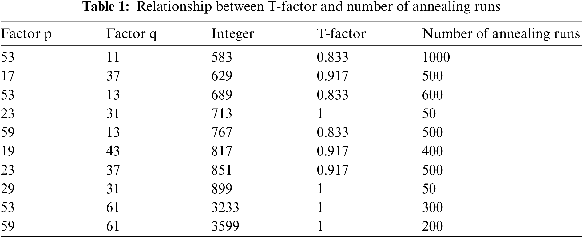
When the T-factor is 1, that is, the multiplier factor can completely fill the multiplier, the number of annealing runs required for integer factorization is very small, within 100 times. When the T-factor is slightly smaller, the number of annealing runs times needed to factor the integers increases exponentially. This result is consistent with our previous conjecture.

In particular, we have factored two larger integers for reference. For the factorization of 3599 and 3233, it can be better seen that the influence of T-factor on integer factorization is far greater than that of the size of the integer itself.

Meanwhile, as mentioned above, within the same search range, the larger the integer is, the easier it is to factor. In Fig. 9, the 6-bit multiplier is used to factor 1517, 1927, 2491 and 3599, respectively. Among them, the number of annealing runs factorization 1517 is 1500, factorization 1927 is 1000, factorization 2491 is 500, factorization 3599 is 200.

Figure 9: The 6-bit multiplier splits large integers

According to Fig. 9, within the same search range, the larger the integer, the smaller the region of potential energy valley, and the fewer the annealing times required for factorization.

It can be concluded that when using quantum annealing to solve the integer factorization problem, the closer the multiplier factors are to each other, the easier it is to factor the integer. According to Eq. (8), if we can judge the range of multiplier factors, then we can greatly reduce the number of quantum annealing required for integer factorization. On this basis, when the number of multipliers and T-factor are the same, the larger the integer is, the easier the factorization will be, which can explain the fluctuation phenomenon caused by traversal factorization at the beginning of this paper.

5  Conclusions and Discussion

Experiments show that the performance of the whole algorithm is affected by setting the bit of the multiplier when using quantum simulated annealing for integer factorization. Experiments show that the integer is easy to be factored when the multiplier is well filled, that is, the highest bit can also be used. If the multiplier is not fully filled, that is, the binary bits of the multiplication factor are less than or much less than the number of the multiplier, the corresponding integer will be difficult to be factored. We attribute this phenomenon to the effect of quantum tunneling in the annealing algorithm. Low potential energy points are densely distributed around the function x=y, so it is easier to obtain optimization of quantum tunneling effects when the binary bits of the two multipliers are similar.

In the current integer factorization methods, the traditional number theory factorization method limits the large integer to q<p<2q, two multiplicators with the same number of digits are the most difficult to be factored, but the study of T-factor shows that when two multiplicators have the same number of digits, it is the easiest to be factored. From this point of view, quantum annealing algorithm makes up for the weakness of traditional number theory methods in integer decomposition.

At the same time, the multiplier factor in integer decomposition is equivalent without any restriction. However, in the experimental results, the output frequencies of the results of these two factors are different. Due to the limited experiments, we can do on the cloud platform, this asymmetry cannot be further explained.

In industry, the annealing process is still the result of the empirical nature of the experiment produced. Furthermore, the indicative significance of the existence of T-factor is far greater than the theoretical value behind it. In future quantum annealing factorization, the padding of the multiplier can be used to roughly predict the number of annealing runs times needed to factor the integer, so as to further reduce the use of qubits.

Furthermore, we consider that the number of annealing runs fluctuates regularly with the increase of integers during ergodic annealing. We can further expand the scope of traversal to obtain a more accurate and wider range of function images. Based on this data, we can take the Fourier transform and predict the range of annealing times needed to factor a range of integers. This is very indicative. When the actual number of annealing runs operations is much larger than this value, we can manually adjust the number of multiplier bits to change the search space to factor the integer more efficiently.

Through reasonable speculation on the experimental results, we think that the annealing times of the traversal annealing image will fluctuate with the increase of the integer, the smaller the integer is, the smaller the period of its fluctuation, the larger the integer is, the larger the period of its fluctuation, and the overall trend of the whole fluctuation function image has a rising trend proportional to the integer size. Therefore, the practical efficiency of quantum annealing for integer factorization needs further consideration.

Acknowledgement: We would like to thank Professor Chao Wang for his encouragements and valuable suggestions on conducting this research.

Funding Statement: This research was funded by the National Natural Science Foundation of China (NSFC) (Grant No. 61972050), and the Open Foundation of State Key Laboratory of Networking and Switching Technology (Beijing University of Posts and Telecommunications) (SKLNST-2020-2-16).

Author Contributions: The author Zhiqi Liu was mainly responsible for the research conception and design of the paper, as well as data collection and processing; Author Xingyu Yan was responsible for the analysis and interpretation of the results; Author Ping Pan helped with further experimental data; Authors Licheng Wang and Shihui Zheng improved the idea structure of the manuscript and the overall article. All authors reviewed the results and approved the final version of the manuscript.

Availability of Data and Materials: Data openly available in a public repository. The data that support the findings of this study are openly available in Github at https://github.com/Leosirius2597/D-Wave-integer-factorization.

Conflicts of Interest: The authors declare that they have no conflicts of interest to report regarding the present study.

References

1. P. L. Montgomery, “A survey of modern integer factorization algorithms,” CWI Quarterly, vol. 7, no. 4, pp. 337–366, 1994. [Google Scholar]

2. R. L. Rivest, A. Shamir and L. Adleman, “A method for obtaining digital signatures and public-key cryptosystems,” Communications of the ACM, vol. 21, no. 2, pp. 120–126, 1978. [Google Scholar]

3. M. Bellare and P. Rogaway, “Optimal asymmetric encryption,” in Advances in Cryptology EUROCRYPT’ 94: Workshop on the Theory and Application of Cryptographic Techniques Perugia, Italy, Springer; pp. 92–111, 1995. [Google Scholar]

4. F. Boudot, P. Gaudry, A. Guillevic, N. Heninger, E. Thomé et al., “Comparing the difficulty of factorization and discrete logarithm: A 240-digit experiment,” in Advances in Cryptology–CRYPTO 2020: 40th Annual Int. Cryptology Conf., Santa Barbara, CA, USA, Springer, pp. 62–91, 2020. [Google Scholar]

5. T. Kleinjung, K. Aoki, J. Franke, A. K. Lenstra, E. Thomé et al., “Factorization of a 768-bit rsa modulus,” in Crypto, Springer, vol. 6223, pp. 333–350, 2010. [Google Scholar]

6. H. Riel, “Quantum computing technology,” in 2021 IEEE Int. Electron Devices Meeting (IEDM), IEEE, pp. 1–3, 2021. [Google Scholar]

7. M. Roetteler, M. Naehrig, K. M. Svore and K. Lauter, “Quantum resource estimates for computing elliptic curve discrete logarithms,” in Int. Conf. on the Theory and Application of Cryptology and Information Security, Springer, pp. 241–270, 2017. [Google Scholar]

8. M. Amico, Z. H. Saleem and M. Kumph, “Experimental study of Shor’s factoring algorithm using the IBM Q experience,” Physical Review A, vol. 100, no. 1, pp. 012305, 2019. [Google Scholar]

9. E. Farhi, J. Goldstone, S. Gutmann, J. Lapan, A. Lundgren et al., “A quantum adiabatic evolution algorithm applied to random instances of an NP-complete problem,” Science, vol. 292, no. 5516, pp. 472–475, 2001. [Google Scholar] [PubMed]

10. S. Jiang, K. A. Britt, A. J. McCaskey, T. S. Humble and S. Kais, “Quantum annealing for prime factorization,” Scientific Reports, vol. 8, no. 1, pp. 1–9, 2018. [Google Scholar]

11. A. Das and B. K. Chakrabarti, “Colloquium: Quantum annealing and analog quantum computation,” Reviews of Modern Physics, vol. 80, no. 3, pp. 1061, 2008. [Google Scholar]

12. W. Peng, B. Wang, F. Hu, Y. Wang, X. Fang et al., “Factoring larger integers with fewer qubits via quantum annealing with optimized parameters,” Science China Physics, Mechanics & Astronomy, vol. 62, no. 6, pp. 1–8, 2019. [Google Scholar]

13. B. Wang, F. Hu, H. Yao and C. Wang, “Prime factorization algorithm based on parameter optimization of Ising model,” Scientific Reports, vol. 10, no. 1, pp. 1–10, 2020. [Google Scholar]

14. S. W. Shin, G. Smith, J. A. Smolin and U. Vazirani, “How “quantum” is the d-wave machine?” arXiv preprint arXiv:1401.7087, 2014. [Google Scholar]

15. D. Saida, M. Hidaka, K. Imafuku and Y. Yamanashi, “Factorization by quantum annealing using superconducting flux qubits implementing a multiplier Hamiltonian,” Scientific Reports, vol. 12, no. 1, pp. 1–8, 2022. [Google Scholar]

16. K. Bharti, A. Cervera-Lierta, T. H. Kyaw, T. Haug, S. Alperin-Lea et al., “Noisy intermediate-scale quantum (NISQ) algorithms,” arXiv preprint arXiv:2101.08448, 2021. [Google Scholar]

17. J. Preskill, “Quantum computing in the nisq era and beyond,” Quantum, vol. 2, pp. 79, 2018. [Google Scholar]

18. B. Yan, Z. Tan, S. Wei, H. Jiang, W. Wang et al., “Factoring integers with sublinear resources on a superconducting quantum processor,” 2022. https://doi.org/10.48550/ARXIV.2212.12372 [Google Scholar] [CrossRef]

19. S. Kirkpatrick, C. D. Gelatt Jr and M. P. Vecchi, “Optimization by simulated annealing,” Science, vol. 220, no. 4598, pp. 671–680, 1983. [Google Scholar] [PubMed]

20. S. Morita and H. Nishimori, “Mathematical foundation of quantum annealing,” Journal of Mathematical Physics, vol. 49, no. 12, pp. 125210, 2008. [Google Scholar]

21. J. H. Shirley, “Solution of the schrödinger equation with a Hamiltonian periodic in time,” Physical Review, vol. 138, no. 4B, pp. 979, 1965. [Google Scholar]

22. M. W. Johnson, M. H. Amin, S. Gildert, T. Lanting, F. Hamze et al., “Quantum annealing with manufactured spins,” Nature, vol. 473, no. 7346, pp. 194–198, 2011. [Google Scholar] [PubMed]

23. H. P. Robertson, “The uncertainty principle,” Physical Review, vol. 34, no. 1, pp. 163, 1929. [Google Scholar]

24. B. M. McCoy and T. T. Wu, The Two-Dimensional Ising Model, Cambridge, MA, USA: Harvard University Press, pp. 31–34, 1973. [Google Scholar]

25. Z. Deng, K. Gao and M. Feng, “Generation of N-qubit W states with rf SQUID qubits by adiabatic passage,” Physical Review A, vol. 74, no. 6, pp. 064303, 2006. [Google Scholar]

26. D. Bertsimas and J. Tsitsiklis, “Simulated annealing,” Statistical Science, vol. 8, no. 1, pp. 10–15, 1993. [Google Scholar]