A Model Average Algorithm for Housing Price Forecast with Evaluation Interpretation

1  Introduction

1.1 Background

One of China’s pillar businesses is the real estate sector. People may make wise home buying decisions and reduce the burden of government regulation by making logical use of a lot of real estate information. Data analysis is being developed in tandem with machine learning. The second-hand housing data can be scientifically processed by the regression model offered by the algorithm and converted into a data format that can be properly evaluated. Based on the evaluation of several regression methods, the AM algorithm continuously improves its statistical capabilities and achieves significant gains in data processing and conclusion prediction.

In the analysis of realistic prediction, establishing a model that is too simple will result in poor model fitting and the conclusion that the prediction is underfitted; establishing a model that is too complex, even though it can fit the existing data well, will cause the issue of overfitting and have an impact on the prediction results. Its goal is to choose several regression models with strong impacts from a variety of perspectives, and then assign a certain weight to each model. The use of the model average approach relies heavily on the weight computation. A weighted mix of model selection and model averaging. Its approach is more thorough for data processing than the model selection method, and it makes it difficult to overlook any model. As a result, several regression algorithms have evolved into a highly useful technique for estimating and researching the cost of used homes. Regression models’ prediction accuracy can exceed 80%, which is very helpful for the real estate sector and allows for very useful decision-making.

1.2 Research Status

Both local and international academics employ a variety of techniques to study and forecast property prices. The two general categories for statistical analysis of house price data are as follows: One is time series data, while the other is panel data (Wang, 2006) [1], (Ni, 2013) [2]. The majority of studies have the following two issues with the aforementioned two techniques: The spatial effect is not taken into account, and there is just one model being used to assess and predict, making it difficult to choose the best prediction model. Some scholars have shown that there is a spatial effect between regional housing prices in China, and the spatial econometric model considers spatial effect to be better than the ordinary Linear Regression model (Yang, 2020) [3]. In the study of housing price forecasting, the majority of researchers opt for the model selection approach, which can choose a relatively optimal pre-selection model in accordance with specific model selection criteria. The pre-selection model will be utilized as a model to produce actual data once it has been chosen. It serves as the foundation for all statistical judgments, similar to placing eggs in a basket (Gong, 2005) [4]. According to Zeng (2020) [5], this approach has some flaws, including instability, high risk, and target deviation. This work explores including the spatial effect in the model and applies the model average approach for empirical analysis of data linked to housing prices on the basis of summarizing the findings of prior research.

2  Related Work

2.1 Linear Regression

The estimation function of the regression model algorithm is established. After obtaining the function, the test data is added to these models, and the model is used to process the data scientifically.

To establish the linear regression model, we need to preprocess the acquired data, and then train the model with relevant algorithms, and then apply the model. Curve fitting is used to analyze the distribution process of the data set, and the fitted curves are finally obtained as straight lines, so linear regression is completed. In addition, the hypothesis function needs to be set in the linear regression, and the hypothesis function adopted in this paper is [5]:

Y=aX+b(1)

Among them, Y is the prediction result of the model (predict house price) to distinguish the real house price, X represents the characteristic factors affecting the change of house price, and a and b represent the parameters of the model.

In the process of data preprocessing, it can be known from the above analysis that the main influencing factor of housing price is housing area information. Data normalization is then performed to prevent the range of these different data ranges from causing the calculated floating point to rise or fall. After observing the distribution characteristics of the data, the normalization operation is completed. By deleting the mean value and dividing the original value range, the value range of these same dimension attributes is scaled and narrowed.

When the loss function is defined, the fluid interface is called to realize variance calculation and obtain variance average, then the input is defined as the predicted value of housing price, while label data is defined, and then the loss value is continued to be calculated. The loss function is optimized by gradient descent [6].

After the model’s initialization, network structure configuration, construction and optimization of the training function, and model training. Prior to using the fluid interface to train and test the model, the actuators are first defined. The trainer can offer a certain optimization method, training hardware location, and related network architecture structure once it has been developed.

2.2 Tree Regression

An evaluation of the net present value, expected value greater than zero probability, and risk assessment of the entire project experiment can be done using a decision tree, a type of prediction algorithm that uses a specific scenario [7], data classification algorithms to determine probability, and finally refactoring to produce a specific decision tree. The feasibility study allows for the evaluation and selection of the best option. By employing its probability analysis properties, the decision tree uses these features to produce decision diagrams.

The Decision Tree’s meaning contains a lot of information, and all of its internal nodes were specifically stated in terms of certain test qualities. Each type of leaf node within the structure might correspond to a variety of different groupings, and each type of branch information is intended to represent an output test.

The Decision Tree must be trained to collect a variety of data, and the data must be used to classify the training sample using a particular algorithm that creates specific properties. These properties or categories must then be implemented to determine these properties or categories, and the resulting classifier produced by machine learning algorithms can provide the final accurate classification of the newly emerged objects [8].

In order to represent the “strong” integrated information, the Random Forest integrates additional learning models based on decision trees, continually collects the “weak” aspects throughout the entire experiment process [9], and then aggregates the output of all information. To lessen potential decision tree flaws, the Random Forest generates various information from a single decision tree. The goal of the random forest is to remove the decision trees with high variation and low deviation in order to create a new model with higher variance and lower variance.

A new tree is used to fit the last complete forecast error when after the completion of the training we get k of the tree, and all need to predict sample points in accordance with the pertinent characteristics of the sample. The XGBoost algorithm obtains the characteristic information of constantly splitting these features to form a tree [10], and each form is learning a new function.

The XGBRegressor() function is immediately invoked for the model accuracy test in order to retrieve the accurate value [11], modify its unique parameters, halt the test once the maximum efficiency is attained, and finally produce the best prediction effect.

2.3 Neural Network

In the process of constructing a neural network, the computational output is described in a way similar to “class and object” [12], and the forward operation function related to forward is written in this paper to complete the calculation process from features and parameters to predicted values.

All the features of the input and the predicted values of the final output are represented by vectors. The input feature x contains 16 components, and the input feature y has only one component. After that, the neural network is constructed. X1 through the model could obtain the training to the representation of specific influencing factors for the prices that can meet the needs of z, the whole experiment actual prices to y, and on the need to complete this distinction specific indicators to measure the predictive value of access to z y actual gap with the real data, this article adopts the method of the mean square error to measure the accurate indicators of the model [13]:

Loss=(y−z)2(2)

In the formula, “Loss” represents the Loss Function, which is used as a measurement index. After that, the loss of samples continued to be calculated. The Network class interface created was used to calculate the predicted value and obtain the loss function, and the dimension information was defined, including the feature vector and the number of samples [14].

By continuing to calculate the gradient, a smaller loss function can be obtained, and the parametric solutions w and b can be found to obtain the minimum value of the loss function.

Fig. 1 gradient descent is used to solve w and b to improve the scientific efficiency of the regression model. To achieve this process, it is necessary to modify the update and training functions in the network and complete the loop iteration to reduce the loss value.

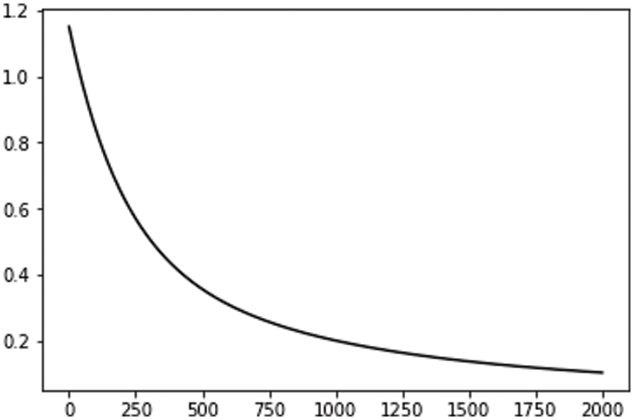
Figure 1: The model was trained 2,000 times

Fig. 2 training neural network, solving target parameters, and training model in the calculation process. The significance of model training is to make the loss function defined above smaller, and finally obtain the parameters so that the loss function can obtain the minimum value. The key part of the training is to find (w, b) vector that minimizes the loss function, and the loss function will change with the change of two parameters [15]:

Loss=Loss(w5,w9)(3)

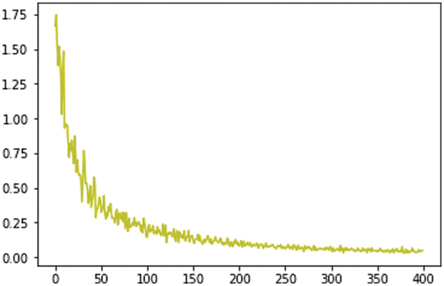
Figure 2: Variation trend of loss function

2.4 Model Average Method

The initial mock test model may offer the best model for researchers, however the one model selected may have flaws such being unreliable, lacking important information, being high risk, and target deviation. The model averaging method was created to address these drawbacks. It is a method of model selection that extends smoothly from estimate and prediction. After the hatchet is weighted by the weight of the candidate models, the first mock exam tosses the helve. The danger of a single model “single throw” is avoided. How to distribute the weight is the most crucial issue [16].

The Model averaging method was first proposed by Buckland in 1997. Its core is the score based on information standards. Since then, many scholars have done more in-depth research on this problem. After that, some scholars proposed a hybrid adaptive regression method-arm method, which is used to combine the estimators of regression function based on the same data. After that, some scholars proposed the arms model averaging method and verified the effectiveness of the method by comparing it with the EBMA method. Hansen (2007) proposed the mallows criterion for selecting weights, that is, the combined model is given appropriate weights by minimizing the mallows criterion, which is proved to be asymptotically optimal in the sense of minimizing the square error of independent data, and proposed mallows model averaging in 2008 (MMA) model averaging method is applied to time series data to further verify the accuracy and effectiveness of mallows criterion [17].

3  Average Model Algorithm

3.1 Algorithm Principle

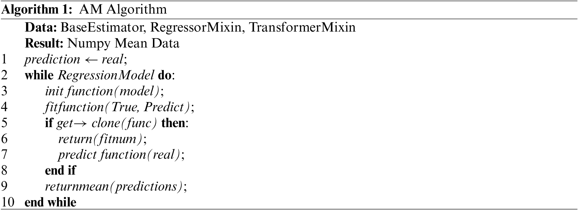
Based on the analysis of relevant regression models, AM Algorithm model is proposed in this paper. The algorithm averages the obtained regression models and then gives weight to each average model by using the comprehensiveness of the method so that the better model will not be overfitted and the sub-optimal model will not be over interfered, to obtain a more scientific house price prediction model [18].

The optimum data properties are first examined once the data has been preprocessed. The outcomes of the prediction are then produced after building the regression model to test the training data. Fig. 3 second, the evaluation function is utilized to assess each model’s ability to forecast, and the regression model’s prediction is displayed.

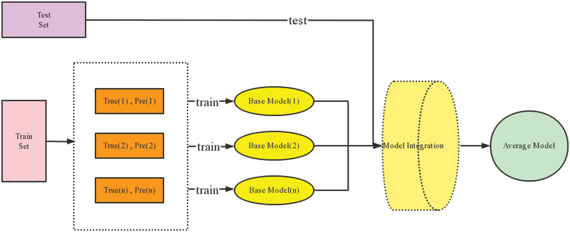
Figure 3: Average model principle

The FMA method is used in the study of the model average, and its core is to correctly define the combination weight, A typical example is the smoothed AIC(S-AIC) and smoothed BIC(S-BIC) methods introduced by Buckland (1997) and others. The final model is obtained by giving appropriate weights to multiple candidate models. The calculation formula for combination weight is [19]:

wk=exp(−xlCk2)∑k∗exp(−xlCk∗2)(4)

In which the xlCk represents AIC and BIC, wk represents the weight corresponding to the w model. The reason for using this weight calculation method is that AIC is an approximate measure of negative double expected log-likelihood, so exp(−xlCk2) is approximately the relative likelihood of model k, where xlCk=AICk−mink∗AICk∗. In addition, from the perspective of information theory, AIC is an approximate unbiased estimation of K-L distance, so exp(−xlCk2) can be regarded as the probability that model k is the minimum K-L distance model. S-AIC and S-BIC are the most commonly used weight selection methods due to their simple operation. The AM Algorithm pseudocode is as follows:

3.2 Algorithm Innovation

The problem can be more thoroughly analyzed using the model averaging method, which also does not readily rule out any viable models. Unfortunately, the quantity of calculations required for the model averaging method would significantly rise when examining multivariable situations. The specific candidate models chosen in the experiment will be averaged in a model with n variables when utilizing the model averaging approach. It can assess data and make predictions with accuracy for the model with fewer variables [20]. As a result, only one model needs to be evenly chosen when employing the model average method, which lessens the computing load [21]. Based on this concept, this research assesses whether the model average approach following principal component regression may increase the prediction accuracy by comparing the prediction errors between models. The outcomes demonstrate that the AM algorithm maximizes the regression error in the prediction degree while obtaining the least prediction error [22].

4  Experiments and Analysis

4.1 Experiment Environment

The operating system used in the experiment is Ubuntu 18.04, the CPU is Intel Xeon(R)CPU E5-2609 v4 @ 1.70 GHz, the GPU is Nvidia 1080Ti with 8 GB of memory, the development language is Python of 3.6.4.

4.2 Data Preprocessing

The datasets are based on second-hand housing data supplied by Baidu Open AI for significant Chinese cities. There is a lot of incorrect information in the obtained data set, and after detailed analysis of the data, the information is classified according to characteristics. The data used by the model algorithm is split into a train set and a test set, with a proportion of 70% and 30%, respectively.

The characteristic values of the gathered datasets are extracted using the machine learning correlation technique, and the correlation between the characteristic values is calculated. The price curve is observed, the correlation feature image is utilized to examine how one characteristic affects the other, to process and evaluate the price, and to ultimately arrive at the prediction result.

The missing value information processing method is used to process the chaotic code anomaly information, and the K-means algorithm is used to fill in the anomaly value. A two-point technique is used to describe data such as elevator, subway, decorating, and tax status, and feature information unrelated to regression classification is immediately eliminated. Additionally, the data are divided into various variables after filling out the form, the continuous data variables are enlarged, and various data kinds are processed by hot code [23].

Numbers of data sets are used above the research process for classification information processing and correlation analysis to determine the factors that influence house price. Then, the feature with the highest correlation is chosen to analyze the change in house price, and various regression models are used to predict the data set. The most innovative aspect of this research was its analysis of how different regression models processed price data sets, its examination of the influences of various characteristics on house prices, its evaluation of the model’s ability to predict prices, and its subsequent adjustment with grid parameters to improve that ability.

Fig. 4 we can determine the possible relationship between price and each feature by analyzing the feature histogram, and the correlation between all elements can be clear and distinct. Each prediction model’s creation is subject to mathematical iteration. Through these mathematical procedures, we can eventually get decent model prediction results while continuously obtaining accurate prediction values.

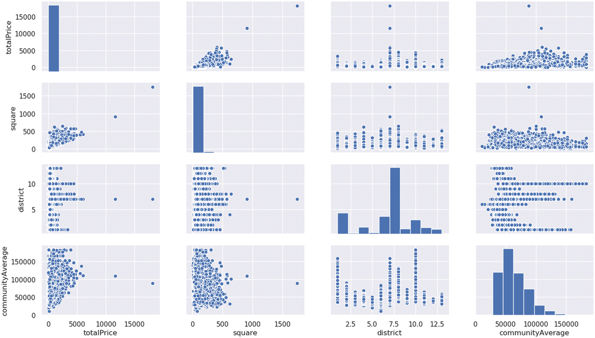
Figure 4: Relationship between totalPrice and features

Fig. 5 it is clear from the thermodynamic diagram that the community average and total price characteristics are more closely linked to the price factors. Future studies will therefore examine these traits, particularly the communityAverage feature. This feature, which will be looked at as the primary influencing factor, allows many models to produce 10% accurate prediction results.

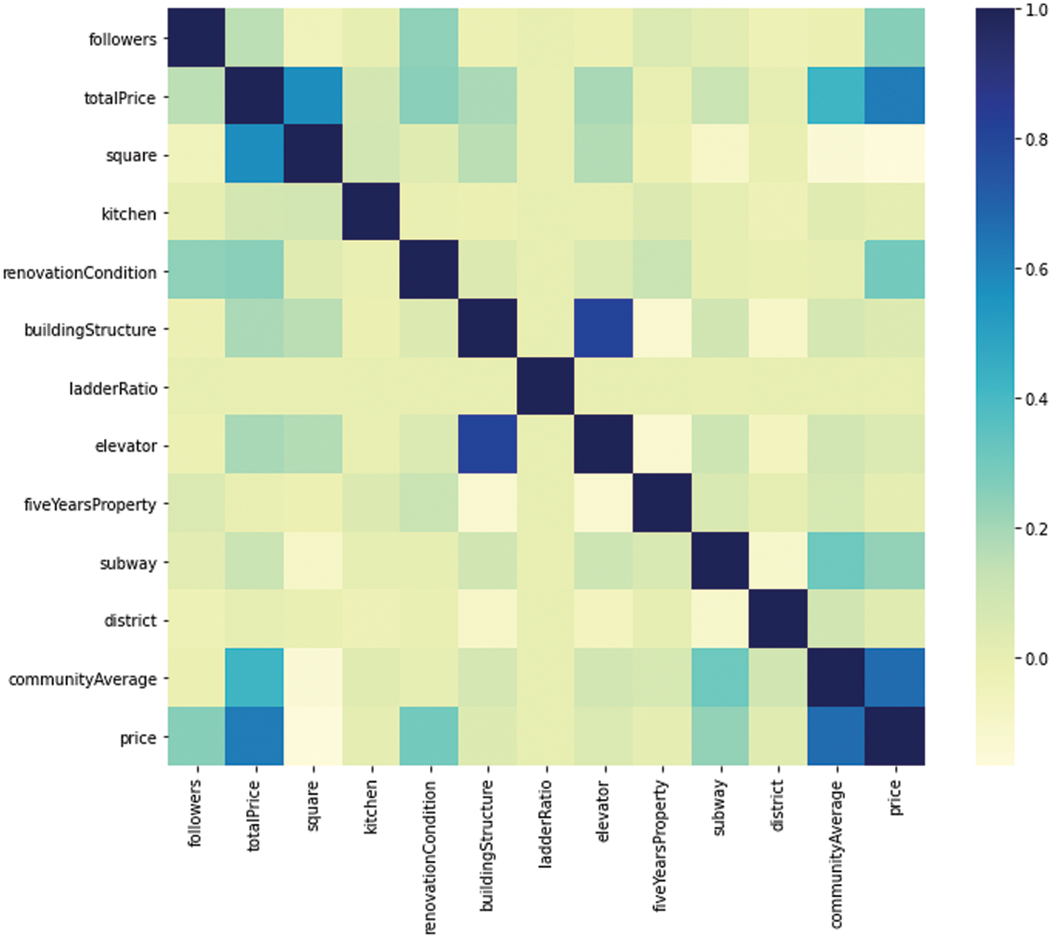
Figure 5: Degree of correlation between features

Fill in the missing values. For example, there is no Subway in the data set in earlier years, so these blanks need to be filled in the Subway column feature to add information without Subway. Perform visual operations on the data and make relevant predictions according to these specific operations.

4.3 Experimental Effect

Specific steps to achieve the prediction Fig. 6:

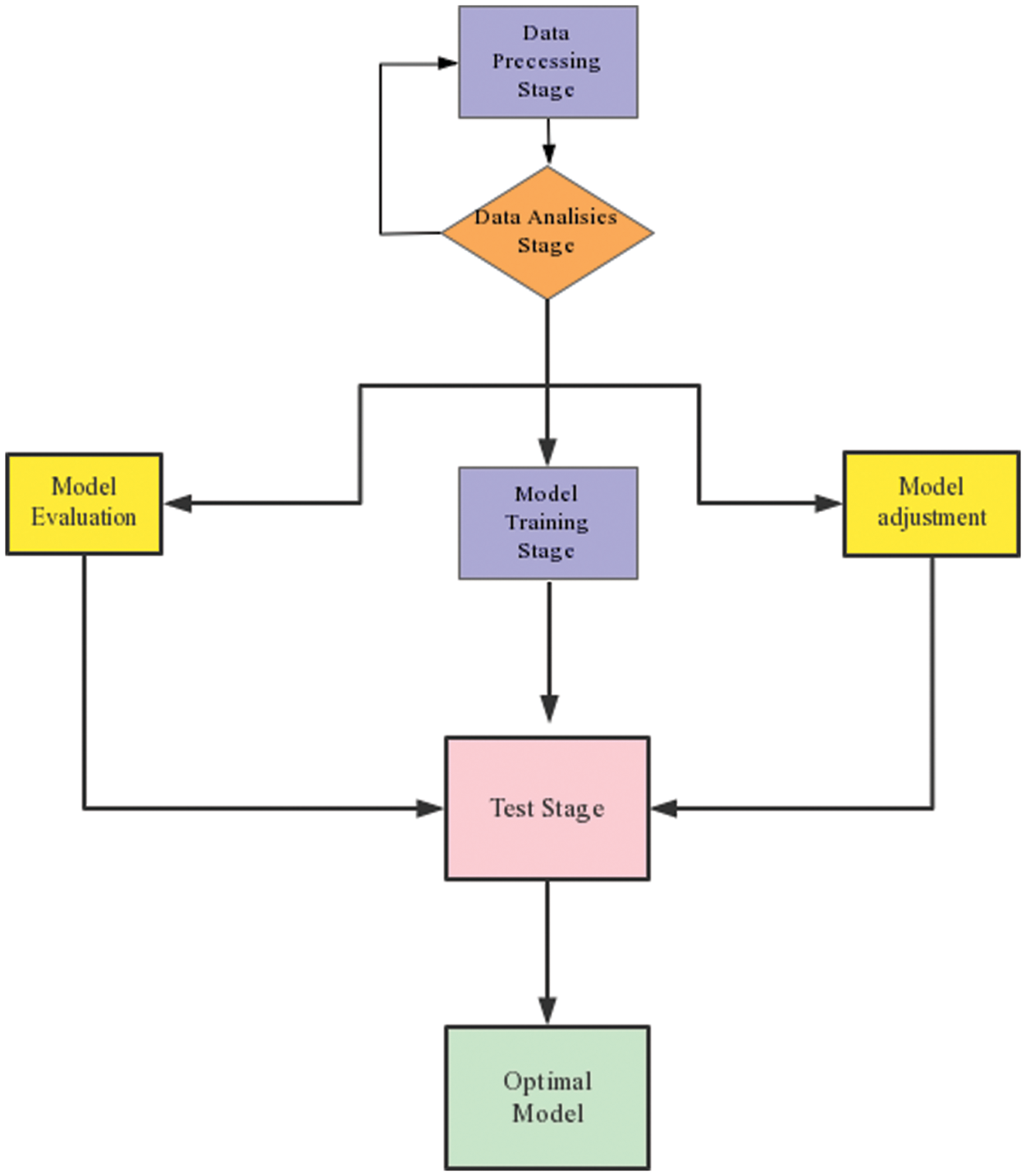
Figure 6: Implementing the best model

In Fig. 7, linear regression model has comprehensive prediction efficiency and good performance. Using the data with the highest one-dimensional correlation to predict and analyze house prices. The analysis of the linear regression model adopts the community average feature, which represents the average price distribution information of the community.

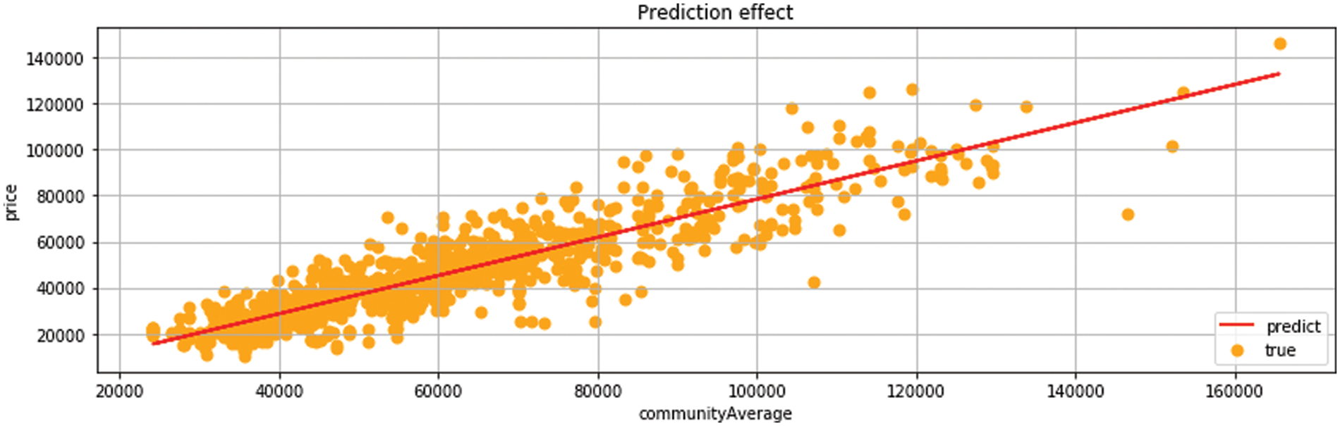
Figure 7: Linear regression

The decision tree is used to train the influence of housing area on price factors. In Fig. 8, the results show that the decision tree is very accurate in the use of a sparse matrix, and the prediction of sparse points is very ideal, but there are still some problems in the prediction of dense points.

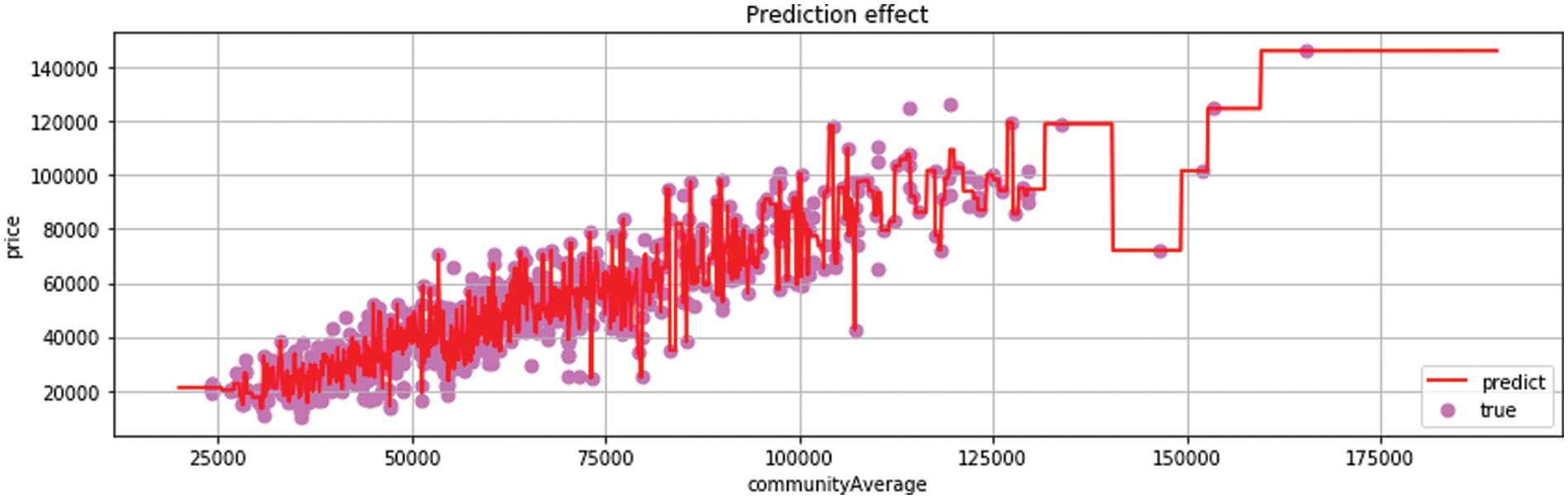
Figure 8: Decision tree regression

Random Forest reduces variance based on decision trees and train multiple sample trees. However, the prediction results of this model are realistic. Sparse points do not obtain the prediction results. For example in Fig. 9, random forests can achieve good results in the field of multi-data prediction. Compared with decision trees, the prediction effect on decentralized data sets is unsatisfactory.

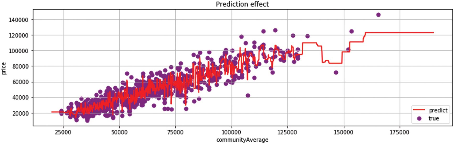
Figure 9: Random forest regression

Random Forest and Decision Tree are the same types of regression algorithms. Fig. 10 extratree and Random Forrest belong to the derivative algorithms of Decision Tree. They generate corresponding regression trees according to the characteristics of information and then find the best segmentation point and the best information data division formula among these regression trees [24].

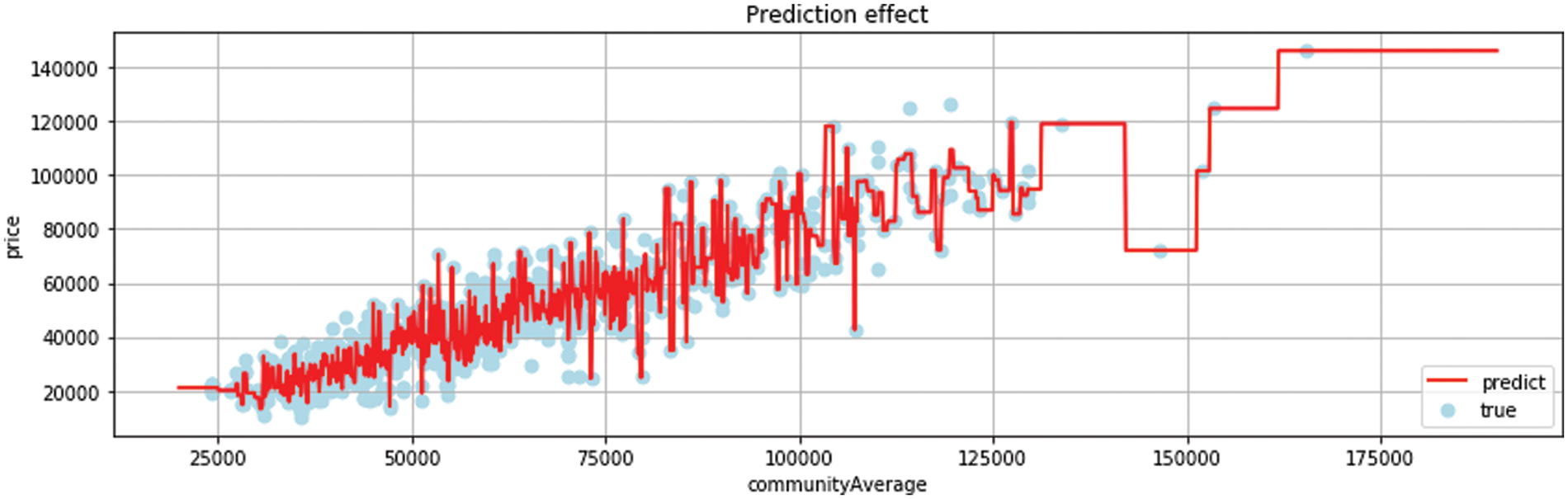
Figure 10: ExtraTree regression

Fig. 11 illustrates how scoring features based on their importance can help identify which characteristics are crucial to the model and how to enhance feature selection based on these features. It is important to note that the district feature and the overall house price feature index rank highly among these aspects, although other features like the bedroom and kitchen might not be the main cause of the high price or might be affected by the supporting infrastructure of the neighborhood. It will be the result of further improved work to determine how these elements impact home pricing [25].

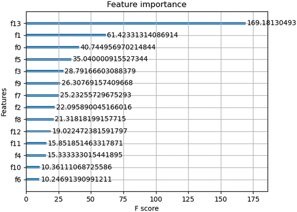
Figure 11: Feature importance

Fig. 12 to achieve a better prediction effect and accurate prediction analysis, the AM algorithm is used to average the models in accordance with the previous model’s prediction effect. Through the algorithm, the weights of each model are assigned, preventing the better model from overfitting and the inferior model from overfitting. Fig. 13 the AM method does not readily give up any candidate model and mixes the candidate models by assigning them a certain weight. As a result, it stays away from the risk of a single model. The main issue is how to distribute weights.

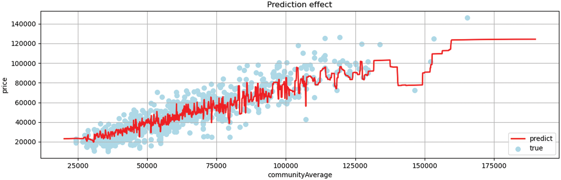
Figure 12: Average model regression

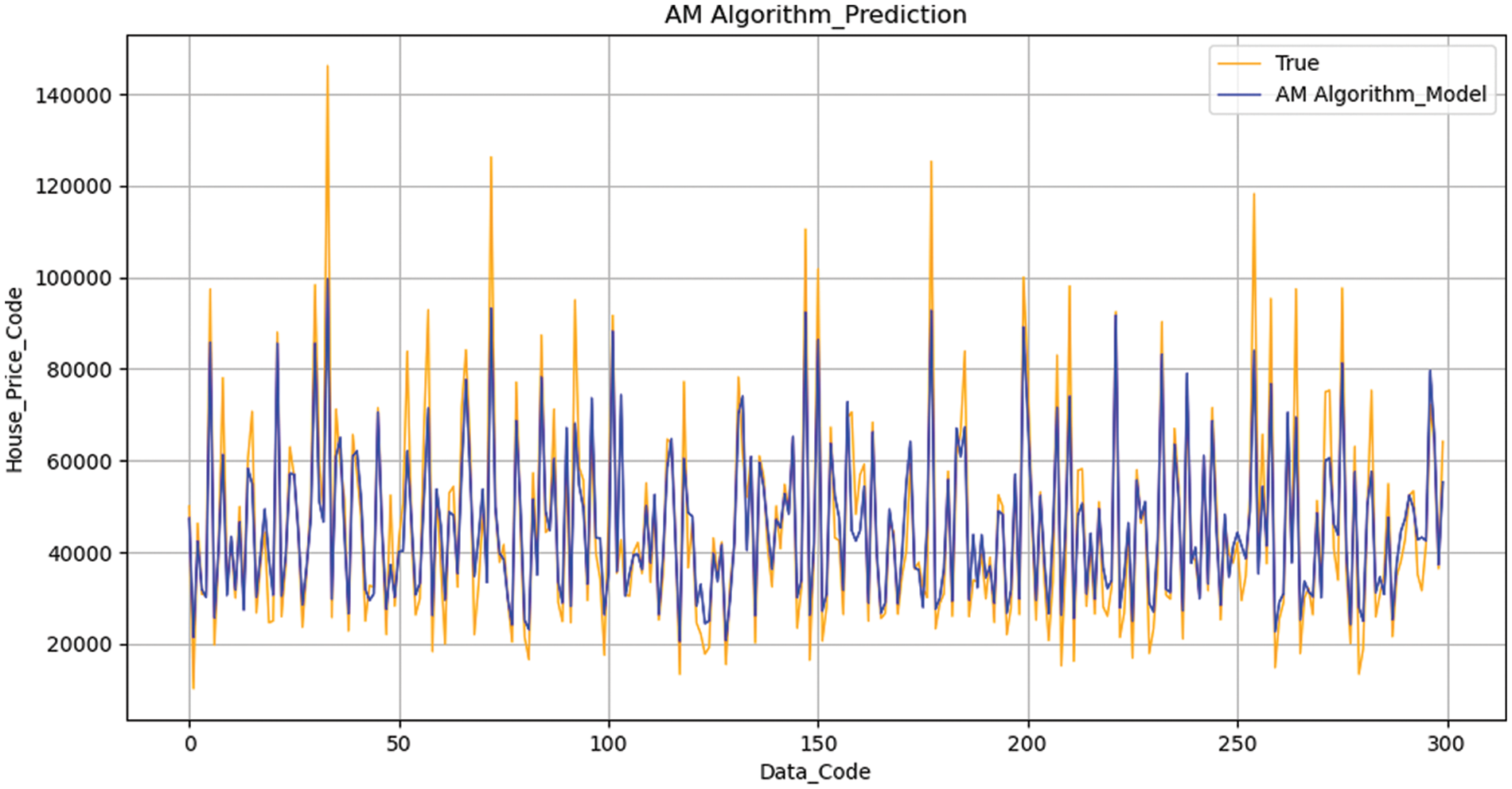
Figure 13: AM Algorithm with optimal parameter adjustment

4.4 Model Evaluation

All the features excluding the unexpected price features are used as the influencing factors of house prices to evaluate the model, which can maximize the prediction effect of the model. The evaluation will train the model with multidimensional data as the basis for the prediction effect of the model.

Expand the continuous variable base and encode the classified variables. The algorithm is standardized. For example, see Table 1, after smoothing the predicted value, SVR algorithm can obtain better prediction results. After the Lasso algorithm is standardized, a negative number exception occurs, and the predicted value is added to the log function for processing to obtain the correct prediction result. The algorithm’s prediction score is ultimately determined by computing the accuracy of the prediction samples after the accuracy is determined by the scoring function.

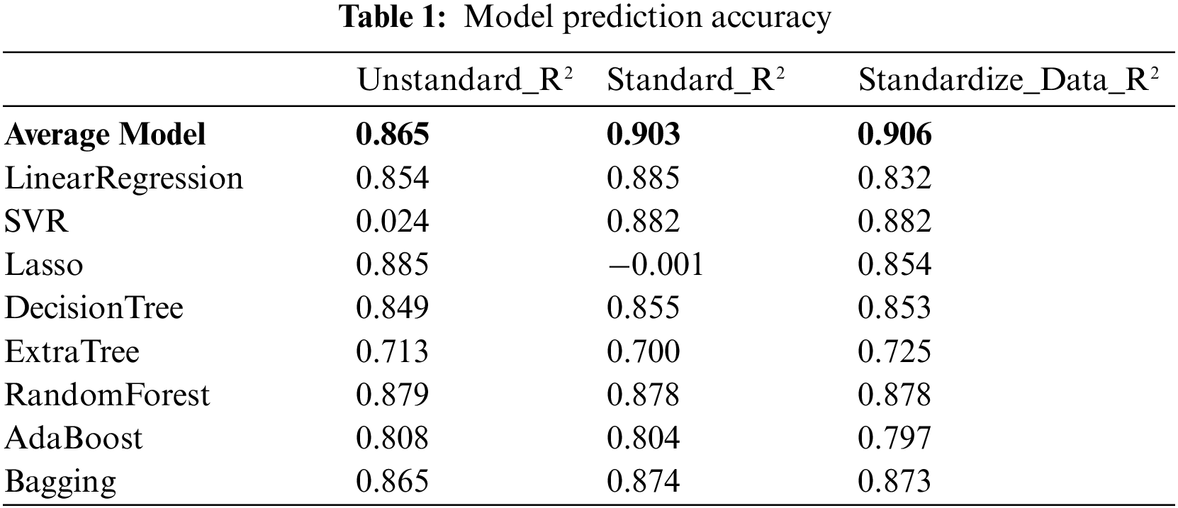
R2 is a statistical measure that represents the proportion of variance of a dependent variable explained by one or more independent variables in the regression model. Correlation shows the strength of the relationship between independent variables and dependent variables, while R2 shows the extent to which the variance of one variable explains the variance of the second variable [26].

R2=1−∑i(yi^−yi)2∑i(yi−y¯)2(5)

where yi represents the real value of house price, yi^ represents the corresponding model prediction value, and y¯ represents the predicted mean value of house price.

The definition of loss function uses the form of a formula to measure the difference between the obtained prediction results and the real data. The smaller difference means better prediction results. For linear models, the loss function often used is the mean square error:

MSE=1n∑i=1n(Y^−Yi)2(6)

For the test set of n obtained data, MSE is the mean information of the square error of n obtained prediction results.

MAE is the average of the absolute value of the error between the observed value and the real value. where yi represents the real value of house price, yi^ represents the corresponding model prediction value.

MAE=∑i=1n|yi^−yi|n(7)

RMSE: the root mean square error, the root mean square deviation represents the sample standard deviation of the difference between the predicted value and the observed value. where yi represents the real value of house price, yi^ represents the corresponding model prediction value.

RMSE(y_real,y_predict)=1n∑i=1n(yi−yi^)2(8)

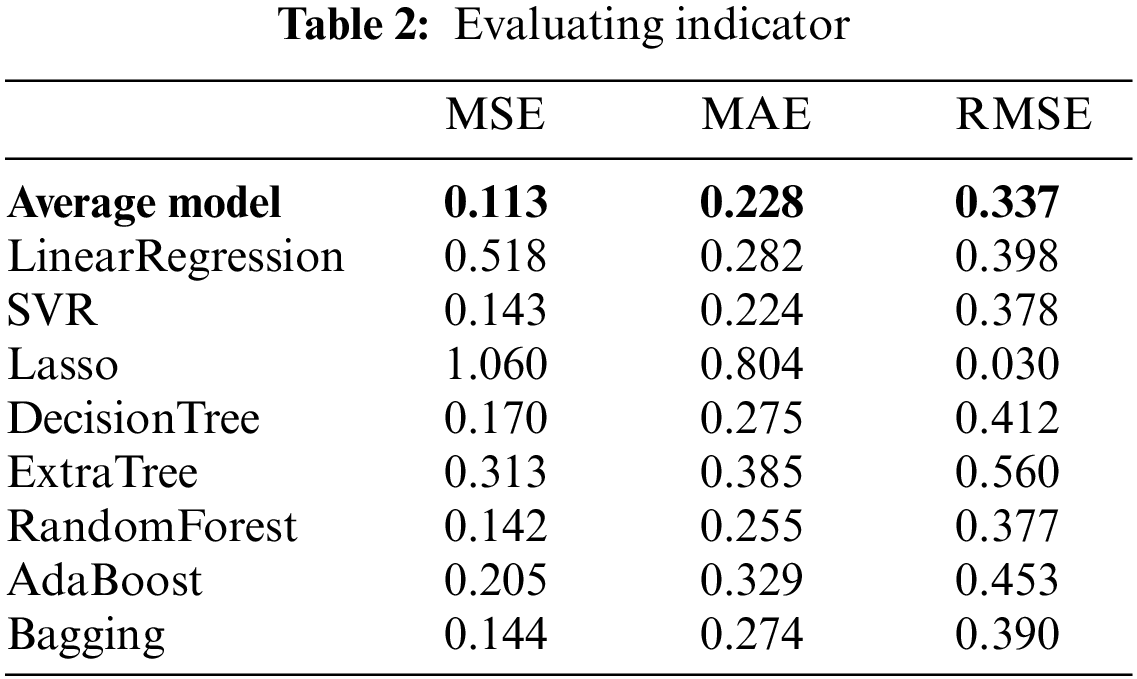
This paper mainly uses MSE and R2 as the evaluation index of the prediction effect of the model. MSE is a measure of estimator quality. It is always non-negative, and a value close to zero is better. Therefore, MSE is very appropriate and effective as an evaluation index. Regression algorithms such as Random Forest and Decision Tree can also obtain an accuracy of more than 80% after parameter adjustment [27].

The mean square error, root mean square error, mean absolute error and R2 value are used as the evaluation function. The smaller the mean error of mean-variance, the better the prediction effect of the model, and the larger the R2 value, the higher the efficiency of the model. It can be seen from Table 2 that AM Algorithm has the smallest MSE value and the largest R2 value, and its score is the highest. It also can be concluded that AM Algorithm has the best effect and high prediction accuracy in the prediction of price characteristics. However, the prediction of Lasso model is abnormal, the R2 value cannot be used as the evaluation index, and the MSE value is high [28], so the prediction effect is the least obvious.

Through the comparison of loss functions, it can be found that among MSE mean square error and MAE, AM algorithm obtains the best effect, obtains the optimal data coupling, and avoids overfitting of Gradient Boost and under fitting information of Linear Regression.

Define the calculation method of the loss function. The KFold [29] function is used for cross- validation, and then the RMSE value is solved for the mean value and continues to converge to obtain the value index, which is used as the evaluation basis. From the final loss function solution, it can be seen that Gradient Boosting also has good results.

After evaluating all the regression models, this paper proposes a new algorithm: AM algorithm, which internally optimizing the models, stacking the predicted results, and then calculates the average value to get a better optimization effect.

By averaging the established regression model, a model with the highest coupling is obtained: am algorithm model. Table 3 after testing and optimizing the error between the real models, the model obtains an evaluation index with the best comprehensive performance, which makes the experimental prediction closer to the real value and reduces the error of overfitting and underfitting [30].

5  Conclusion

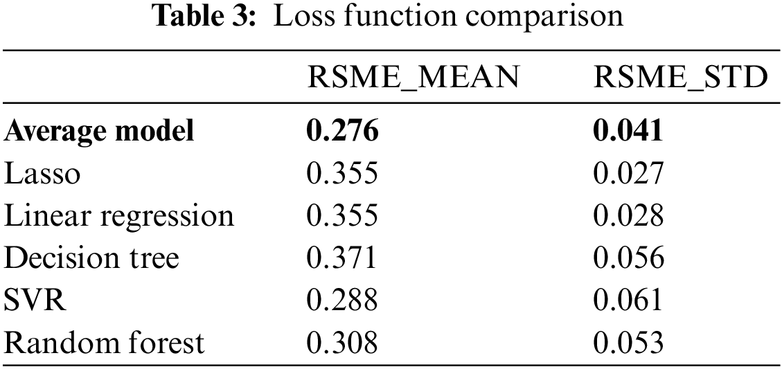
The AM algorithm has the most potent integrated algorithm ability and has a better impact on price prediction, according to the examination of the final prediction effect and error function. The AM method has a smoother processing mode and a better fitting effect on standard data, regardless of the implementation mode, parameter use, or data processing.

The AM algorithm can process the model with the minimum gradient according to the information in the data set in the experiment on the data sets for second-hand housing, and utilize the mean sum approach to get good prediction results for various regression models. Additionally, the AM approach can enhance the coupling strength of the model and adapt well to the error handling techniques used in different regression models. This technique has a wide range of applications and will not readily discard any candidate model to produce more complete results. Only the model average approach and principal component analysis method are combined in this work. Presumably, many traditional methods can be combined with AM algorithm method, which may achieve better results in analyzing and predicting practical problems.

To assess and forecast the second-hand house sales price index, the study combines the time series model with the model selection and model average approach. The AM algorithm is established, the autocorrelation function and partial autocorrelation function of the data are observed, many candidate models are obtained, the MSE and R2 values of each model are calculated and compared, the better model is chosen, and a new model is established using the AM method. This new model is then used to predict the second-hand housing sales price index, the prediction errors of which are compared, and it is ultimately decided that the AM algorithm is the most accurate. In addition, the AM algorithm proposed in this paper has many contributions in the field of regression prediction in machine learning, including being able to be flexibly applied to the regression analysis of stock development trend, the regression analysis of weather index change trend, and so on. Moreover, the implementation efficiency of the algorithm is high and takes up less resources, and the algorithm such as comparison set learning is more simple and effective.

Funding Statement: This work was supported in part by Sichuan Science and Technology Program (Grant No. 2022YFG0174) and in part by the Sichuan Gas Turbine Research Institute stability support project of China Aero Engine Group Co., Ltd (Grant No. GJCZ-0034-19). (Corresponding author: Yong Zhou).

Conflicts of Interest: The authors declare that they have no conflicts of interest to report regarding the present study.

References

1. Z. Z. Wang, “Research and implementation of price forecasting model based on machine learning,” M.S. Dissertation, Chang’an University, China, 2018. [Google Scholar]

2. D. Ni, “Research on real estate Pricing method based on data mining,” M.S. Dissertation, Dalian University of Technology, China, 2013. [Google Scholar]

3. S. Yang, “An empirical study of housing price prediction in China based on model average,” M.S. Dissertation, Yunnan University of Finance and Economics, China, 2020. [Google Scholar]

4. H. L. Gong, “Empirical research on prediction model of second-hand house price in Wuhan based on XGBoost algorithm,” M.S. Dissertation, Central China Normal University, China, 2018. [Google Scholar]

5. T. Zeng, “Research on housing price prediction model based on machine learning,” M.S. Dissertation, Southwest University of Science and Technology, China, 2020. [Google Scholar]

6. M. Liu, “Housing price prediction analysis based on Network search data,” M.S. Dissertation, Shandong University, China, 2018. [Google Scholar]

7. X. Wang, “Research on regional housing price forecasting model and its application in China based on web search,” M.S. Dissertation, Nanjing University, China, 2016. [Google Scholar]

8. D. Zheng, Z. Ran, Z. Liu, L. Li and L. Tian, “An efficient bar code image recognition algorithm for sorting system,” Computers, Materials & Continua, vol. 64, no. 3, pp. 1885–1895, 2020. [Google Scholar]

9. Y. Wang, “A study on the prediction of housing price based on machine learning algorithm,” Beijing University of Technology(Natural Science Edition), vol. 11, no. 2, pp. 230–288, 2019. [Google Scholar]

10. R. M. Valadez, “The housing bubble and the GDP: A correlation perspective,” Business and Economics, vol. 3, no. 3, pp. 66–70, 2010. [Google Scholar]

11. A. A. N. Meidani, M. Zabihi and M. Ashena, “House prices, economic output, and inflflation interactions in Iran,” Applied Economics, vol. 3, no. 1, pp. 5–10, 2011. [Google Scholar]

12. J. Cheng, R. M. Xu, X. Y. Tang, V. S. Sheng and C. T. Cai, “An abnormal network flow feature sequence prediction approach for DDoS attacks detection in big data environment,” Computers, Materials & Continua, vol. 55, no. 1, pp. 95–119, 2018. [Google Scholar]

13. Z. -H. Chen, C. -T. Tsai, S. -M. Yuan, S. -H. Chou and J. Chern, “Big data: Open data and realty website analysis,” in The 8th Int. Conf. on Ubi-Media Computing, Colombo, Sri Lanka, vol. 56, no. 24, pp. 84–88, 2015. [Google Scholar]

14. W. -T. Lee, J. Chen and K. Chen, “Determination of housing price in Taipei City using fuzzy adaptive networks,” in Int. Multiconference of Engineers and Computer Scientists, Hong Kong, vol. 12, no. 3, pp. 13–15, 2013. [Google Scholar]

15. D. Zheng, X. Tang, X. Wu, K. Zhang, C. Lu et al., “Surge fault detection of aeroengines based on fusion neural network,” Intelligent Automation & Soft Computing, vol. 29, no. 3, pp. 815–826, 2021. [Google Scholar]

16. C. Chang, “Design and implementation of real estate price forecasting system based on multi-modal information fusion,” M.S. Dissertation, Beijing University of Posts and Telecommunications, China, 2019. [Google Scholar]

17. J. Zhu, “Design and implementation of second-hand housing data analysis system,” M.S. Dissertation, Southwest Jiaotong University, China, 2017. [Google Scholar]

18. X. Y. Huang, Python implements house price forecasting, In: J. Tao (Ed.China: CSDN, 2018. https://blog.csdn.net/huangxiaoyun1900/article/details/82229708 [Google Scholar]

19. F. H. Cai, Thirteen regression models predict house prices, In: J. Tao (Ed.China: CSDN, 2019. https://blog.csdn.net/weixin_41779359/article/details/88782343 [Google Scholar]

20. S. Ma, “Research and application of second-hand housing price prediction model based on LSTM,” M.S. Dissertation, Zhengzhou University, China, 2020. [Google Scholar]

21. H. Dai, “Research on price prediction of second-hand housing transactions in beijing based on stacking theory,” M.S. Dissertation, University of Science and Technology Liaoning, China, 2019. [Google Scholar]

22. Y. Li, “Research on price prediction of second-hand house in Beijing based on BP neural network,” M.S. Dissertation, Capital University of Economics and Business, China, 2018. [Google Scholar]

23. J. Sun, “Real estate big data analysis system based on Elasticsearch,” M.S. Dissertation, Xidian University, China, 2019. [Google Scholar]

24. R. Liang, “Research on housing rent in shenzhen based on machine learning model,” M.S. Dissertation, Central China Normal University, China, 2020. [Google Scholar]

25. Q. Liu, “Housing price Prediction analysis based on Network search data,” M.S. Dissertation, Chongqing University, China, 2019. [Google Scholar]

26. X. Bai, “Prediction and analysis of house prices in Qingdao Based on model selection and model average method,” M.S. Dissertation, Central University for Nationalities, China, 2021. [Google Scholar]

27. F. Wang, “Research on stock market risk warning based on deep learning method,” M.S. Dissertation, North China University of Technology, China, 2021. [Google Scholar]

28. Z. Y. Lu, “Research on price prediction and comparison of stock index futures based on machine learning algorithm,” M.S. Dissertation, Zhejiang University, China, 2020. [Google Scholar]

29. K. Xing, D. E. Henson, D. Chen and L. Sheng, “A clustering-based approach to predict outcome in cancer patients,” in Machine Learning and Applications, 2007. ICMLA 2007. Sixth Int. Conf. on IEEE Computer Society, Cincinnati, OH, USA, 2007. [Google Scholar]

30. J. Erfurt, W. -Q. Lim, H. Schwarz, D. Marpe and T. Wiegand, “Multiple feature-based classifications adaptive loop filter,” in Picture Coding Symp. (PCS), San Francisco, CA, USA, 2018. [Google Scholar]