Journal of Quantum Computing DOI:10.32604/jqc.2022.027683
Article

Study on Quantum Finance Algorithm: Quantum Monte Carlo Algorithm based on European Option Pricing

Jian-Guo Hu1,*, Shao-Yi Wu1,*, Yi Yang1, Qin-Sheng Zhu1, Xiao-Yu Li1 and Shan Yang2

1School of Physics, University of Electronic Science and Technology of China, Chengdu, 610054, China
2Department of Chemistry, Physics and Atmospheric Science, Jackson State University, Jackson, MS, USA
*Corresponding Authors: Jian-Guo Hu. Email: shimukouziyue@163.com; Shao-Yi Wu. Email: wushaoyi@uestc.edu.c
Received: 06 January 2022; Accepted: 29 April 2022

Abstract: As one of the major methods for the simulation of option pricing, Monte Carlo method assumes random fluctuations in the distribution of asset prices. Under certain uncertainties process, different evolution paths could be simulated so as to finally yield the expectation value of the asset price, which requires a lot of simulations to ensure the accuracy based on huge and expensive calculations. In order to solve the above computational problem, quantum Monte Carlo (QMC) has been established and applied in the relevant systems such as European call options. In this work, both MC and QM methods are adopted to simulate European call options. Based on the preparation of quantum states in QMC algorithm and the construction of quantum circuits by simulating a quantum hardware environment on a traditional computer, the amplitude estimation (AE) algorithm is found to play a secondary role in accelerating the pricing of European options. More importantly, the payoff function and the time required for the simulation in QMC method show some improvements than those in MC method.

Keywords: Monte carlo method (MC); option pricing; quantum monte carlo (QMC); amplitude estimation (AE); payoff function

1  Introduction

An option refers to a contract that gives the holder the right to purchase or sell an asset at a fixed price (strike price) prior to a specific date (exercise window). In simple terms, The strike price is a fixed price, and the time range is also a single point in time. However, exotic variants can lead to multiple underlying assets, that is to say, the execution price can be a function with many execution windows. Option is not only a profitable tool but also the core of various hedging strategies [1].

Due to the randomness of the defined parameters, it is feasible but difficult to calculate the fair value [2]. Many numerical methods, especially Monte Carlo (MC) method has been commonly used in pricing system due to its flexibility and ability to handle generically stochastic parameters [3,4]. Despite many advantages in option pricing and wide application in financial field, MC method usually demands a lot of computation resources to ensure the accuracy of the estimated value.

As is known, quantum computers [5] based on quantum mechanics provide new methods to solve a large number of computational problems, and have a wide range of applications in the fields of quantum finance [6], quantum chemistry [7–10] and machine learning [11–13]. Quantum finance, a field with many computationally hard problems, may benefit from quantum computing. Recently developed applications of gate-based quantum computing in finance include calculation of risk measures and pricing of financial derivatives [14]. Many quantum computing methods emerged in the optimization of portfolio investment, risk measurement calculation and derivative pricing. All these applications are based on the Amplitude Estimation algorithm [15], by estimating a parameter with a convergence rate of 1/M, with the number M of quantum samples [14] and representing a theoretically quadratic speed-up compared to classical MC methods.

This article mainly focuses on the application of MC and QMC methods in European call options and further analysis for the certain examples. In the second section, the path based on the simulation with MC method is found similar to Brownian motion. The asset price on the exercise day is also introduced, with the basic principles of MC. And the relevant probability distribution on a quantum computer is also illustrated, with the basic principles of QMC. In the third section, the algorithm structure and some code examples of the MC and QMC methods are described, by giving a specific example of European call options. In the fourth section, the simulation results of MC and QMC algorithms are illustrated and discussed, and the advantages and disadvantages are analyzed and compared for both methods. Since the classic MC algorithm is relatively mature, this article stresses mainly on the AE and QMC algorithms.

2  Classical and Quantum Monte Carlo Principles

2.1 Classical Monte Carlo Principles

The theoretical basis of Monte Carlo method is probability theory and mathematical statistics. The method is to assume that the asset price distribution is of random fluctuations. If the fluctuation process is known, different random paths can be simulated and yield an asset value. When this process is performed for several times, the obtained result could be regarded as an optimal asset value distribution, which can bring forward the desired asset price. The dominant advantage of MC method is that the error convergence rate does not depend on the dimensionality of the problem. However, accurate pricing demands MC method to perform millions of simulations with huge calculations [16].

Below we introduce the stock price volatility model, European option prices in efficient markets, with the Black-Scholes equation [16]:

∂V∂t+rS∂V∂S+12σ2S2∂2V∂S2−rV=0(1)

where r is the risk-free interest rate. S is the stock price. σ is a constant representing the stock price, and V is the option price.

Set W as the standard one-dimensional Brownian motion under the known probability measure P. The volatility of the grid, u(S(t), t), is the stock price return rate, and S(t) is the stock z price at time t.

dSt=μStdt+σSdW(2)

In the above expression, dW represents white noise, with a character in the meaning of mean square, dW≈εdt,(dW)2≈dt, ε obeys the normal distribution N(0, 1).

By using the Ito’s lemma [17], we get:

dln⁡St=12∂2(ln⁡St)∂St2σ2St2dt+∂(ln⁡St)∂StμStdt+∂(ln⁡St)∂StσStdzt(3)

Assuming that the stock price at the initial moment is S0, the solution to Eq. (2) under the risk-neutral measure can be written as [18]:

ST=S0exp⁡[(r−σ22)T+σTε](4)

In a risk-neutral world, r is the risk-free interest rate, a is the annualized standard deviation of stock returns, and T is the annualized expiration time. The key variable for controlling ST is ε∼N(0,1). By sampling ε∼N(0,1), the stock price can be simulated.

Only European options is considered here. Since they can only be exercised on the exercise date (T), the strike price of the underlying asset can be set as K. Then at time T on the exercise day, CT and PT represent a European call option and a European put option, respectively:

CT=max(0,ST−K)PT=max(0,K−ST)(5)

According to the principle of risk-neutral pricing (i.e., the expected rate of return of the underlying asset is the risk-free interest rate), application of MC simulation in option pricing needs a risk-neutral environment. The future cash flow is discounted by the risk-free interest rate, and It is only the transformation of probability space. Because it is not mentioned that investors are risk-neutral, so there is no need to assume investors’ risk preference. Therefore, on day t, the price of the option is the discounted value of the expected return from the expiration date T:

C0=PV[ E(max(0,ST−K)) ]=e−r(T−t)E(max(0,ST−K))P0=PV[ E(max(0,K−ST)) ]=e−r(T−t)E(max(0,K−ST))(6)

Simulate N times ST, calculate payoff=max(ST−K,0), find the average value of N payoffs and then discount it, yielding the call options price.

2.2 Quantum Monte Carlo Principles

The three building blocks are required to price options on a gate-based quantum computer. (1) Represents the probability distribution P describing the evolution of the random variable X={x1,x2,…,xn}, (2) Construct a circuit for calculating the payoff f(X). (3) Calculate the expectation value of the payoff Ep[f(x)].

2.2.1 Amplitude Estimation

Quantum Amplitude Estimation (QAE) is a fundamental quantum algorithm with the potential to achieve a quadratic speedup for many applications that are classically solved with MC simulation. Assumes a unitary operator A acting on (n + 1) qubits such that [19]:

A|0⟩n|0⟩=1−α|ψ0⟩n|0⟩+α|ψ1⟩n|1⟩(7)

Here |ψ0⟩n and |ψ1⟩n are two normalized states, where a∈[0,1] is unknown.

For European option contracts, the random variables involved represent the possible value Si that the underlying asset can take and the corresponding probability pi of realization. For options with payment value f , the A operator can lead to the following states:

∑i=02n−11−f(si)pi|si⟩|0⟩+∑i=02n−1f(si)pi|si⟩|1⟩(8)

Comparing Eqs. (7) and (8), we can obtain :

a=∑i=02n−1f(si)pi=E[F(s)](9)

This shows that AE can allow us to calculate the price of the underlying asset on the exercise date of the option and create the state of Eq. (8) to express the return of the option as a quantum circuit, which can be described in the follows.

The quantum circuit may be illustrated in Fig. 1, where H denotes a Hadamard gate and F† the inverse QFT [20,21].

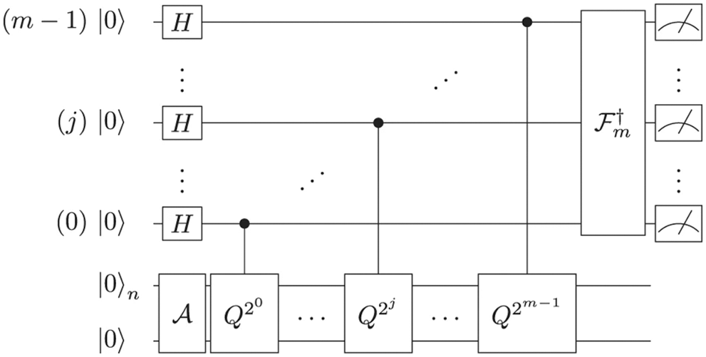
Figure 1: The quantum circuit of AE

2.2.2 Distribution Loading

The first step in option pricing is to build a circuit that takes the probability distribution implicit in the possible future asset prices and loads it into the quantum register. Its amplitude represents the corresponding probability and each ground state represents a possible value. Given an n qubit register, asset prices {Si} for i ∈ {0, …, 2n − 1} and corresponding probabilities {pi}, the distribution loading module can create the state [14]

|ψ⟩n=∑i=02n−1pi|si⟩n.(10)

The Black-Scholes-Merton (BSM) model [22,23] in option pricing indicates that the price of the underlying stock has a lognormal distribution with constant volatility on the exercise date. quantum computers based on gate circuits can efficiently load log-concave probability distributions (such as the log-normal distribution of the BSM model).

One can create the operator A so that a=E[f(x)] to obtain the expectation value of the linear function f of a random X with AE [19].

3  Algorithm Analysis and Implementation

Here we make algorithm analysis on the construction process of the two algorithms as an example. Suppose there is a stock option with a maturity of six months, the underlying asset stock price is 4.36 yuan, the option strike price is 5 yuan, the annualized risk-free interest rate and annualized volatility are 3% and 20%, respectively. Simulation is performed using MC method to find the price of call options and put options with loop iterations of 20,0000 times.

3.1 Classical Monte Carlo Algorithm

The MC method for option pricing is generally divided into the following steps:

(1)   Divide the time interval [0, T] before the expiration date into multiple equidistant Δt sub-intervals.

(2)   Carry out I simulations, i∈{1,2,…,I}, with each simulation having loop of M sub-intervals. At each interval point t∈{Δt,2Δt,3Δt,…,MΔt}, take a random number Zt(i). According to discretization of Eq. (4), ST can be calculated. Then the intrinsic value of the option CT at time T can be calculated.

(3)   According to the first simulation, the expiration value (C0) of the option could be determined.

3.2 Quantum Monte Carlo Algorithm

The QMC method for option pricing is generally divided into the following steps:

(1)   Build uncertainty model

First of all, we need to prepare the quantum state. A circuit is used to load a log-normal state randomly distributed into the quantum state. The distribution is truncated to a given interval [low, high], and discretized using 2n grid points, where n represents the number of qubits used. The unitary operator corresponding to the circuit factory is implemented as follows:

|0⟩n→|ψ⟩n=∑i=02n−1pi|i⟩n(11)

The probability corresponding to the truncated discrete distribution is pi, and i is mapped to the right interval using the affine map:

{0,…,2n−1}∍i→high−low2n−1∗i+low∈[low,high](12)

(2)   Building the payment function

For the spot price of the expiring ST < K, the return function is equal to zero, and then linearly increases. The implementation of this module relies on a comparator. If ST ≥ K, it flips an auxiliary qubit from |0⟩ to |1⟩. This auxiliary qubit is used to control the linear part of the payment function.

Approximation can be made for the linear part here. Apply sin2(y+π/4)≈y+1/2 for small |y|, and consider a given approximation rescaling factor capprox∈[0,1] and x∈[0,1], thus

sin2(π/2∗capprox∗(x−1/2)+π/4)≈π/2∗capprox∗(x−1/2)+1/2(13)

for small capprox.

Based on the above process, an operator can be constructed to act as controlled Y-rotations.

|x⟩|0⟩→|x⟩(cos⁡(a∗x+b)|0⟩+sin⁡(a∗x+b)|1⟩)(14)

Eventually, we focus on the measuring probability of |1⟩ in the last qubit, corresponding to sin2(a∗x+b). Together with the above approximation, this allows to approximate the values of interest. The smaller the chosen capprox, the better the approximation. However, in view of the estimation for a property scaled by capprox, the number of evaluation qubits m needs to be adjusted accordingly.

(3)   Obtain the expectation value of a linear function f for a random variable X

One can obtain the expectation value of a linear function f for a random variable X with AE by creating the operator A such that a = E[f(X)].

4  Results and Discussion

4.1 Classical Monte Carlo Simulation Results

Fig. 2 shows the first 30 simulation paths of MC method, with each path obtained from the discretization of Eq. (4) based on the previous sub-interval. So does the next subinterval. It is found from the example that we need to simulate 200,000 times, and the discount value of the simulated option can be obtained from Eq. (6) on the exercise date.

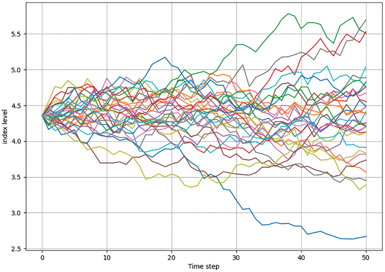
Figure 2: Classic Monte Carlo top 30 simulation paths

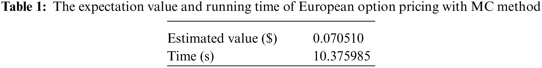
Tab. 1 describes the results of the computer simulation. Through MC method, the discounted value of the option on the exercise date is 0.070510$, and the computer time is 10.375985 s. Despite the short simulation time of 200,000 times, option pricing generally requires tens of millions of simulations and hence a lot of time.

4.2 Quantum Monte Carlo Simulation Results

Fig. 3 describes the spot price and probability line chart simulated with QMC algorithm on the exercise day. The x-axis is the spot price of the day, and the y-axis is the corresponding probability. The figure shows that the probability is the highest for the spot price 4.156, but it is fewer than the strike price (k = 5) on the day the option was purchased, indicating CT = 0 from Eq. (5). From Fig. 3, CT is greater than zero for the spot price of 5.235, 5.774 and 6.313, which can be regarded as profitable.

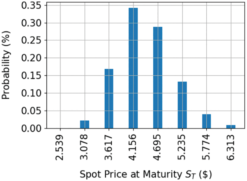
Figure 3: Example price distribution at maturity loaded in a quantum register

Fig. 4 is the payoff function image, describing the discounted price along with the spot price on the day of the exercise. When the spot price is lower than the stock price (K), the payoff is 0. As the spot price is greater than K, the payoff can show increasing trend.

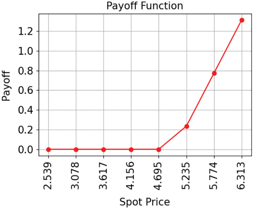
Figure 4: Plot exact payoff function (evaluated on the grid of the uncertainty model)

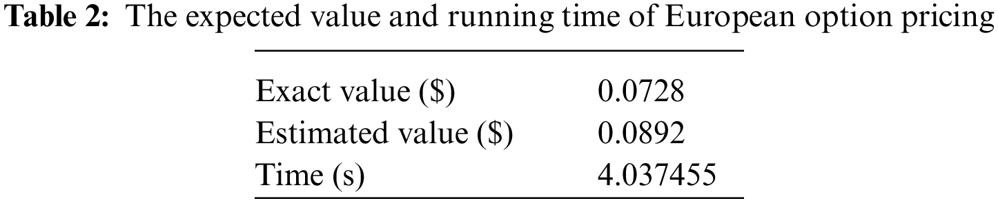
Tab. 2 is the simulation result of QMC algorithm. Based on the uncertainty model, the accurate expectation value (normalized between [0, 1]) is obtained, together with the required simulation time.

4.3 Comparative Analysis of MC and QMC

From the above example of European call options, the path of the option can be simulated, and the discounted price and the time required for computer simulation are obtained with MC method. we can see that AE allows us to compute the undiscounted price of an option given a way to represent the option’s payoff as a quantum circuit and create the state. The above example can also be analyzed with QMC method, which would reduce the time required for the results with amplitude estimation (AE). The MC algorithm reveals that the expectation value of European options after six months is 0.070510, while that with QMC algorithm is 0.0892, which are comparable with each other. As for the simulation time, MC method takes the simulations of 200,000 times, much larger than different from QMC. Obviously, QMC method realizes considerable time reduction with respect to MC method by more than 60%. In fact, the number of random numbers that need to be processed will significantly increase with increasing the simulation time. So, the advantage of reduction of time required by using QMC method would be expected more and more important for such systems as European call options with increasing complicacy.

5  Conclusion

This article concerns mainly with the brief introduction for MC and QMC algorithms, especially their applications in the example of a specific European call option as well as comparisons for the two methods. Based on the simulations, the advantage of MC method in the error convergence rate independent of the dimensionality of the problem is verified. However, QMC algorithm shows significant advantage in the problems requiring relatively accurate simulation with a lot of calculations such as present option pricing. An option pricing and quantum circuit is proposed by a gate-based quantum computer, and the pricing of options depends on AE. Compared with MC method, QMC allows secondary acceleration. In view of the current resources of quantum computers available, the actual quantum hardware remains to be tested, and the algorithm is also necessary to be optimized according to the realistic situation. Therefore, it seems that QMC still has a lot of space for development.

Acknowledgement: This work was financially supported by the National Natural Science Foundation of China Granted No. 11764028. One of the authors (Jian-Guo Hu) would also like to thank Tian-tian Li for his helpful suggestions.

Funding Statement: The authors received no specific funding for this study.

Conflicts of Interest: The authors declare that they have no conflicts of interest to report regarding the present study.

References

 1.  T. Kariya and R. Y. Liu, “Options, futures and other derivatives,” in Asset Pricing, Boston, MA: Springer, pp. 9–26, 2003. [Google Scholar]

 2.  F. Black and M. Scholes, “The pricing of options and corporate liabilities,” Journal of Political Economy, vol. 81, no. 3, pp. 637–654, 1973. [Google Scholar]

 3.  P. P. Boyle, “Options: A Monte Carlo approach,” Journal of Financial Economics, vol. 4, no. 3, pp. 323–338, 1977. [Google Scholar]

 4.  P. Glasserman, Monte Carlo Methods in Financial Engineering, New York: Springer-Verlag, 2003. [Google Scholar]

 5.  M. A. Nielsen and I. Chuang, Quantum Computation and Quantum Information, USA: Cambridge University Press, 2002. [Online]. Available: https://doi.org/10.1119/1.1463744. [Google Scholar]

 6.  R. Orus, S. Mugel and E. Lizaso, “Quantum computing for finance: Overview and prospects,” Reviews in Physics, vol. 4, no. 1, pp. 100028, 2019. [Google Scholar]

 7.  A. Kandala, A. Mezzacapo, K. Temme, M. Takita and M. Brink, “Hardware efficient variational quantum eigensolver for small molecules and quantum magnets,” Nature, vol. 549, no. 7671, pp. 242–246, 2017. [Google Scholar]

 8.  A. Kandala, K. Temme, A. D. Corcoles, A. Mezzacapo, J. M. Chow et al., “Error mitigation extends the computational reach of a noisy quantum processor,” Nature, vol. 567, no. 1, pp. 491–495, 2019. [Google Scholar]

 9.  N. Moll, P. Barkoutsos, L. S. Bishop, J. M. Chow, A. Cross et al., “Quantum optimization using variational algorithms on nearterm quantum devices,” Quantum Science and Technology, vol. 3, no. 3, pp. 030503, 2017. [Google Scholar]

10. M. Ganzhorn, D. J. Egger, P. Barkoutsos, P. Ollitrault, G. Salis et al., “Gate-efficient simulation of molecular eigenstates on a quantum computer,” Physical Review Applied, vol. 11, no. 1, pp. 044092, 2019. [Google Scholar]

11. S. Lloyd, M. Mohseni and P. Rebentrost, “Quantum principal component analysis,” Nature Physics, vol. 10, no. 9, pp. 631–633, 2014. [Google Scholar]

12. J. Biamonte, P. Wittek, N. Pancotti, P. Rebentrost, N. Wiebe et al., “Quantum machine learning,” Nature, vol. 549, no. 1, pp. 195–202, 2017. [Google Scholar]

13. V. Havlicek, A. D. Corcoles, K. Temme, A. W. Harrow, A. Kandala et al., “Supervised learning with quantum-enhanced feature spaces,” Nature, vol. 567, no. 1, pp. 209–212, 2019. [Google Scholar]

14. N. Stamatopoulos, D. J. Egger, Y. Sun, C. Zoufal, R. Iten et al., “Option pricing using quantum computers,” Quantum, vol. 4, no. 1, pp. 291–302, 2020. [Google Scholar]

15. G. Brassard, P. Hoyer, M. Mosca and A. Tapp, “Quantum amplitude amplification and estimation,” Contemporary Mathematics, vol. 305, no. 1, pp. 53–74, 2000. [Google Scholar]

16. S. Fadugba, C. Nwozo and T. Babalola, “The comparative study of finite difference method and Monte Carlo method for pricing European option,” Mathematical Theory & Modeling, vol. 2, no. 4, pp. 60–67, 2012. [Google Scholar]

17. U. Hassler, “Ito’s Lemma,” in Stochastic Processes and Calculus, Cham: Springer, pp. 239–258, 2016. [Google Scholar]

18. P. Pellizzari, “Efficient Monte Carlo pricing of European options using mean value control variates,” Decisions in Economics and Finance, vol. 24, no. 1, pp. 107–126, 2001. [Google Scholar]

19. D. Grinko, J. Gacon, C. Zoufal and S. Woerner, “Iterative quantum amplitude estimation,” npj Quantum Information, vol. 7, no. 52, pp. 1–12, 2021. [Google Scholar]

20. S. Woerner and D. J. Egger, “Quantum risk analysis,” npj Quantum Information, vol. 5, no. 15, pp. 1–16, 2019. [Google Scholar]

21. P. Rebentrost, B. Gupt and T. R. Bromley, “Quantum computational finance: Monte Carlo pricing of financial derivatives,” Physical Review A, vol. 98, no. 1, pp. 022321, 2018. [Google Scholar]

22. A. O. Petters and X. Y. Dong, “The BSM model and European option pricing,” in An Introduction to Mathematical Finance with Applications, New York, USA: Springer, pp. 383–475, 2016. [Google Scholar]

23. C. B. Hunzinger and C. C. A. Labuschagne, “An overview of the Black-Scholes-Merton model after the 2008 credit crisis,” Studies in Computational Intelligence, vol. 583, no. 1, pp. 41–52, 2015. [Google Scholar]

This work is licensed under a Creative Commons Attribution 4.0 International License, which permits unrestricted use, distribution, and reproduction in any medium, provided the original work is properly cited.