Application of Machine Learning For Prediction Dental Material Wear

1  INTRODUCTION

Recent years have seen a significant increase in scientific interest in bio-tribology. The field of bio-tribology research is very complex and encompasses a variety of scientific fields. Numerous studies on dental wear, which is a section of bio-tribology, have been undertaken during the past two decades. Finding appropriate dental restorative materials is the current focus of dental tribology. It has been found that dental composites are appropriate materials for dental restoration. The usage of composite materials for restorative purpose has increased significantly for the few decades as a result of their great aesthetics, ability to be in bind with the tooth structures, and requires an amalgam replacement.[1]

Paediatric dentistry as well as restorative dentistry frequently makes use of composite resins. Most of the composite materials that are now on the market are constructed using Bis-GMA, UDMA, or TEGDMA. Bis-GMA is most often used due to its higher molecular dimension and chemical constitution. The monomer TEGDMA is usually applied for diluting Bis-GMA. The properties such as, viscosity, toughness, and filler loading are improved by adding UDMA. A silane coupling agent is coated on inorganic filler particles to improve photoactivation.[2-5]

Various factors such as, temperature, intraoral mechanical loading, corrosion, etc., are influencing the tribological as well as mechanical characteristics of composites. Material loss from the interface of two interacting surfaces is known as wear. Different wear mechanisms are involved in intraoral tribology, which are corrosive wear, fatigue wear, two/three-body wear. Wear may be due to an individual mechanism or due to combination of various mechanisms. Resistance to hardness and two or three-body wear of restorative composites were studied.[6] Current improvements in study of wear mechanisms, chewing simulation testing and root causes material failures in the oral surrounding were analyzed elaborately.[7] Dental composite must be age-resistant in order to be used in the mouth for an extended period of time. Aging resistance of dental composites inside the mouth depends upon its surface roughness, solubility and water absorption. Effect of artificial aging on surface roughness and hardness of composite materials were studied.Similar behavior was observed using the conditions of distilled water and artificial saliva.[8] Different dental composites were tested for wear under distilled water and with poppy seeds as a third body under variable chewing forces.[9] Mechanical characteristics are influenced when composites are subjected to thermal cycling. Effect of thermal cycle on wear of composites was studied by using a chewing simulator.[10] A smooth surface improves aesthetics while lowering plaque retention and surface discolouration. Smooth surface improves the comfort of the patient.[11-12] Viscoelastic characteristics of resin composites are affected by a large range of temperatures. This may lead to change the properties (e.g. micro-leakage, rigidity) of the dental materials.[13] Wear of antagonist composite materials was investigated by performing different chewing tests.[14]

Digitalization has considerably increased in the dental industry during the last 10 to 20 years. Over the past many years, machine learning (ML) techniques have increased, especially in various science and engineering domains. Artificial neural network (ANN) technique has also been applied by various researchers for prediction of tribological characteristics, such as wear and coefficient of friction of tested materials.[15,16] Standard ML algorithms were also applied by various researchers for prediction of tribological parameters. Performance models were improved by adjusting the parametric values related to the model.[17] In most of developed countries the knowledge of dental or medical technology is of no use because of vast application of software technology for example, artificial intelligence (AI). It reduces time, cost and human errors also.[18] Machine learning has been widely applied in periapical lesions, dental caries, oral cancer, orthodontics and dental implants.[19] An algorithm was developed for predicting when a patient needs dental implants.[20] ML algorithm was designed for tooth decay prediction in adults.[21] AI based applications in dentistry, its challenges and solutions to these challenges were discussed.[22] Degree of tooth surface decay was predicted with an accuracy of 5% using genetic algorithm and artificial neural network.[23] Outcome of endodontic microsurgery was predicted using a trained model involving different variables. Gradient boosting model outperformed better than the Random Forest model.[24] An AI model using deep learning was developed for identifying dental plaque and find out the model accuracy in diagnosing.[25] A comprehensive analysis of AI and ML in dentistry was carried out. It provided the community with a thorough understanding of all the accomplishments made possible by these tools and technology.[26]

Cause of deterioration of tooth in many people is habit of chewing tobacco, paan and paan masala. Hence the main objective of this work is to perform an in-vitro test for evaluating the effect of tobacco immersion on the wear of composites. This study also aimed to predict the wear characteristics of dental composites while submerged in tobacco using various ML models in AI.

2  EXPERIMENT

Two-body wear and three-body wear are two basic mechanical principles that can be investigated using various wear simulation methods. A variety of two-body wear simulators have been used to simulate clinical wear. These simulators include the Taber abraser, rotating counter sample two-body wear machine, sliding two-body wear machine, fretting test, abrasive disc, oscillatory wear test, and pin-on-disc tribometer. In addition, several three-body wear mechanisms have been developed to simulate masticatory abrasion. The ACTA wear machine, the BIOMAT wear simulator are some of these simulators. In this study, an In-vitro test (ASTM G99-04) was performed on a pin-on-disc tribometer for quantifying the wear of four composite material specimens pre-immersed in a tobacco solution.[27] These composite materials are available in syringes of 3 to 4 gm. Cylindrical specimens (10 mm X 30 mm) were built by using a mold of elastomer material. A layer of dental composite ranging from 1 to 3 mm was poured into the mold, subsequently the layer was condensed and polymerized with an LED curing light. Based on the information provided in the production cataloge, the curing time was chosen. The specimens were subsequently immersed in distilled water over seven days. The rotating disc was of stainless steel material (grade 316L). Required surface roughness (0.8 micron) on pin specimen and disc was achieved by polishing by a sand paper (600-grit).[28] In order to replicate the actual oral environment, track width, disc speed and test duration were taken as 50 mm, 100 rpm and 10 minutes respectively.[29]

The solution used to immerse the specimens was made by combining tobacco and artificial saliva in equal quantities. pH of the solution was measured by a pH meter.[30] Throughout the immersion period, the pH was attained constant. Compositions of material are summarized in Table 1. Wear of specimens were calculated after 2 days, 3.5 days, 6 days, 15 days and 30 days of immersion which is equivalent to the actual interaction period of material with the tobacco for 1 week, 2 weeks, 1 month, 2 months, and 5 months, respectively. Preliminary baseline readings were taken for un-immersed specimens in artificial saliva. Few authors studied the wear of dental composites for different immersion periods.[31-32]

3  MACHINE LEARNING MODELS

Problems of supervised learning are the issues where the datasets consist of both dependent as well as independent variables. Few machine learning models depend upon resemblance measure distance among data points which are not scaling up to the mark under higher dimensions. Because of this these ML techniques do not perform well when the problem is more complex.

The algorithm is arranged with a set of training data and a target function. The algorithm finds a predictor which diminishes the error. The objective of an algorithm is to find a predictor which reduces the error. Empirical risk minimization (ERM) is a principle in which a predictor hs can be found by using a learning paradigm which diminishes the training error Es(g). The training error is presented in Eq. (1) given below.[33]

Es(g)=|{j∈{1……,m} g(zj)≠uj}|m (1)

Eq. (1) is based on the learning theory.[34] One simple strategy is to minimize the error by memorizing the training data, although this method performs badly for untested data.[35] Applying the ERM rule to a limited region in selecting the hypothesis class of predictors is a typical method for solving the problem. The following sections provide a brief discussion on prediction models which are based on learning theory.

3.1. Ada Boost algorithm

To increase the effectiveness of binary classifiers, the adaptive boosting (AdaBoost) algorithm was developed as an ensemble learning technique. For improving the efficiency of the model, it tries to merge many weak learners to make a strong learner.[36] This algorithm has to train the samples in each of the iterations and set the weights of classifiers that perform poorly. Each sample is assigned with identical weights for creating a weak learner. This weak learner has to undergo training using the data which are weighted. A coefficient is chosen depending on the effectiveness of the classifier having weak learning. The weights are increased for misclassified points and reduced for correctly classified points when the weights are incorrect. To get a weak classifier for the fresh weighted data, the weak learning algorithms are then performed once more. Once the maximum number of iterations has been achieved or all the data points have been accurately categorized, the process is repeated.

3.2. Cat Boost algorithm

Boosting is the recent trend of machine learning technique which is most successfully developed. Despite having been created initially for classification issues, it has been effectively used with regression issues.[37] Boosting techniques can improve capacity of weak learners to approximate accurate predictors while navigating challenging and complex classes. The CatBoost method was developed to address issues including gradient bias and prediction shift.[38,39] It is a perfectly symmetrical tree model, which reduces overfitting and boosts accuracy.[40]

In order to significantly improve feature dimensions by taking advantage of relationships between features, it makes use of a number of category features that work together. The technique includes a prior distribution term P (given in Eq. (2)), which reduces the noise effect and low frequency data and hence improves the capacity of the model to generalize.[39]

dli=∑i=1p−1[dσi,l=dσp,l]Zσi+a.P∑i=1p−1[dσi,l=dσi,l]+a (2)

3.3. Gradient Boosting algorithm

The Gradient Boosting technique employs a succession of tree models and learns from the errors made by previous models. Predictions are created in machine learning by “boosting” an ensemble of inefficient prediction models.[41] By using a gradient descent loss function to compare the updated estimate to the initial estimate, the errors are reduced. A final model is produced by combining all initial estimations with the appropriate weights. The gradient descent loss function is expressed as follows:

fM(xj)=∑mMγmhm(xj) (3)

Where, hm is the weak learner, M is number of trees and γm is the scaling factor which considers the effect of a tree in the model.

3.4. Random Forest algorithm

This algorithm chooses the outcome depending on the predictions given by the decision trees. It makes predictions by averaging the results from different trees. The accuracy of the result increases with the number of trees. The disadvantages of the decision tree method are overcome by the random forest algorithm. Accuracy is improved, and over-fitting of dataset is reduced. Table 2 provides a description of all the parameters that were employed in this study.

3.5. Evaluation of ML models

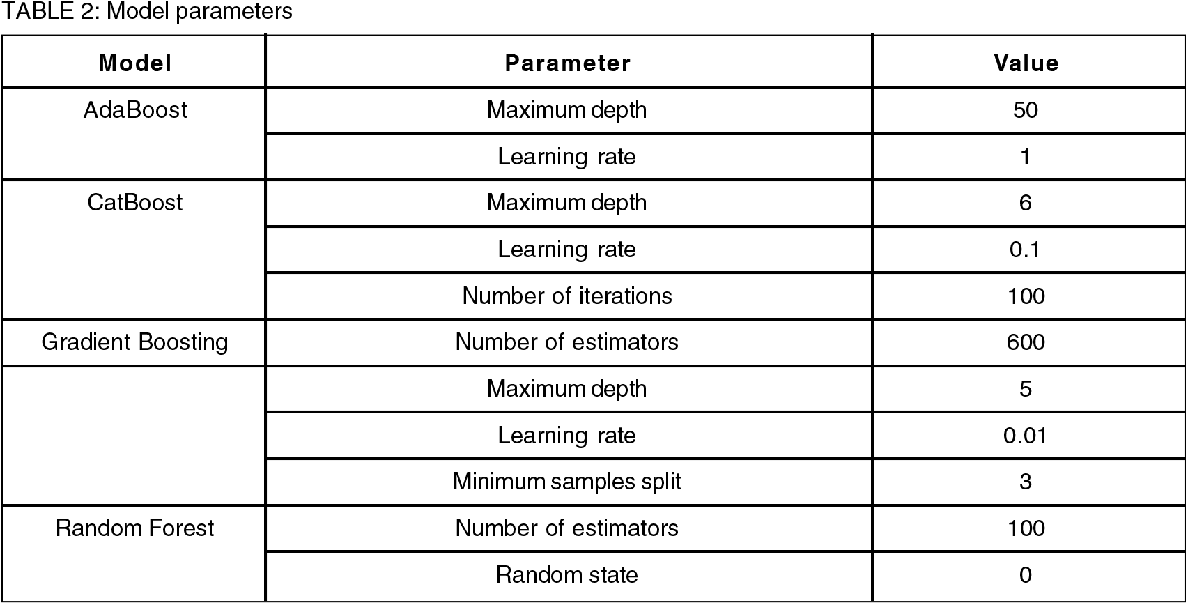
The ML models were formed by writing a Python code using the libraries (Scikit-learn, Numpy and Pandas). Seventy two numbers of data was used which was split with percentages of training data and test data as 80% and 20% respectively. Model fitting was done for the data. Models were gauged by using four parameters: root mean square error (RMSE), regression coefficient (R2), mean absolute error (MAE) and average absolute deviation percentage (AAD%) which are defined below.

MAE=1n∑i=1n|Sexp−Spred| (4)

RMSE=1n∑i=1n(Sexp−Spred)2 (5)

R2=∑i=1n(Sexp−S¯pred)2−∑i=1N(Sexp−S¯pred)2∑i=1N(Sexp−S¯pred)2 (6)

AAD %=1n∑i=1n(|Sexp−SpredSexp|)×100 (7)

A frequently used parameter for evaluating ANN networks and optimizing ANN weight coefficient initial values is the RMSE parameter. RMSE should approach to zero and R2 value should approach to one for better results. The level of the correlation existing between predicted and experimental data is measured by the R2 value.[42,43]

4  RESULTS AND DISCUSSIONS

4.1. Feature selection

Mutual information (MI) technique is implemented for the selection of features from of the input variables. Fig. 1 presents the feature selection plot. MI is a statistical process for assessing the coincidence between two datasets. Feature selection was done by applying the Gradient Boosting algorithm. Absolute values of each feature are not of importance, but the comparative value between the features has the importance. “Days of immersion” is the most significant of the three features (material (mat), load, and days of immersion) as shown in Fig. 1. However, it can be seen that the two features, “load” and “material,” hardly differ in their F scores. As a result, these two features will almost have the same impact on the dependent parameter.

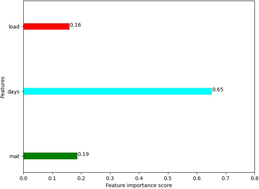
Fig. 1: Feature selection by MI technique

4.2. Predicted wear Vs experimental wear

The experimental Vs predicted wear plot by applying the AdBoost model is presented in Fig. 2. The errors are within a margin of ±15%. The AdaBoost model yields an MAE, RMSE, R2 value and AAD% of 0.7111, 0.8460, 0.9207 and 7.83% respectively. Among all the four models considered, the AdaBoost model shows the highest values of MAE, RMSE and AAD%, but the lowest R2 value.

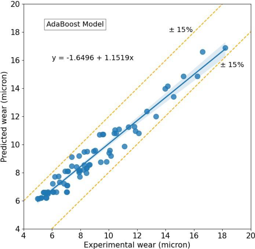
Fig. 2: Predicted wear using AdaBoost model versus experimental wear

Accuracy of wear prediction using CatBoost model w.r.t experimental wear is shown in Fig.3. The errors are within a margin of ±5%, which is very less. This model produces an MAE, RMSE, R2 value and AAD% of 0.0773, 0.1130, 0.9985, and 0.88% respectively.

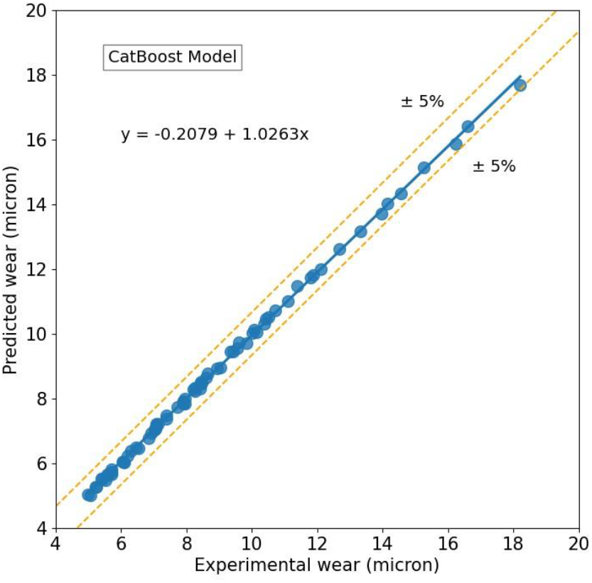
Fig. 3: Predicted wear using CatBoost model versus experimental wear

The experimental Vs predicted wear plot by applying the Gradient Boosting model is shown in Fig. 4. The margin of error is ±5%. This model gives an MAE, RMSE, R2 value and AAD% of 0.0771, 0.0957, 0.9989 and 0.88% respectively. The CatBoost model and Gradient Boosting show the lowest values of MAE and RMSE, but highest R2 value among the four models considered.

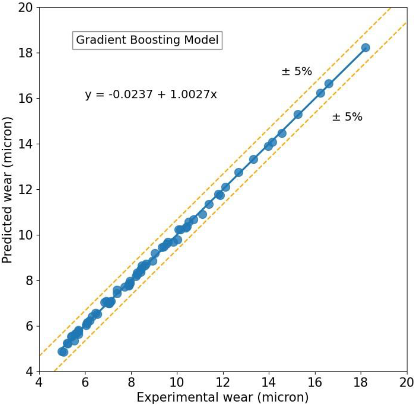
Fig. 4: Predicted wear using Gradient Boosting model versus experimental wear

Plot of experimental Vs predicted wear applying Random forest model is given in fig. 5. The errors are within ±5%. The values of MSE, RMSE, R2 and AAD are 0.2199, 0.3013, 0.9899, and 2.51% respectively. The MAE, RMSE, R2 value and AAD% for all the models used are given in Table 3.

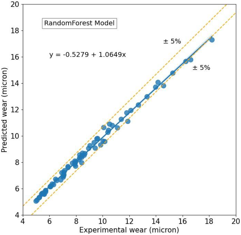
Fig. 5: Predicted wear using Random Forest model versus experimental wear

Fig. 6 shows the comparative wear plot of using all the ML models. It demonstrates how closely the predicted wear obtained by the Gradient Boosting model, CatBoost model and Random forest model match well with the experimental. However, the wear predicted by AdaBoost greatly deviates from the test results.

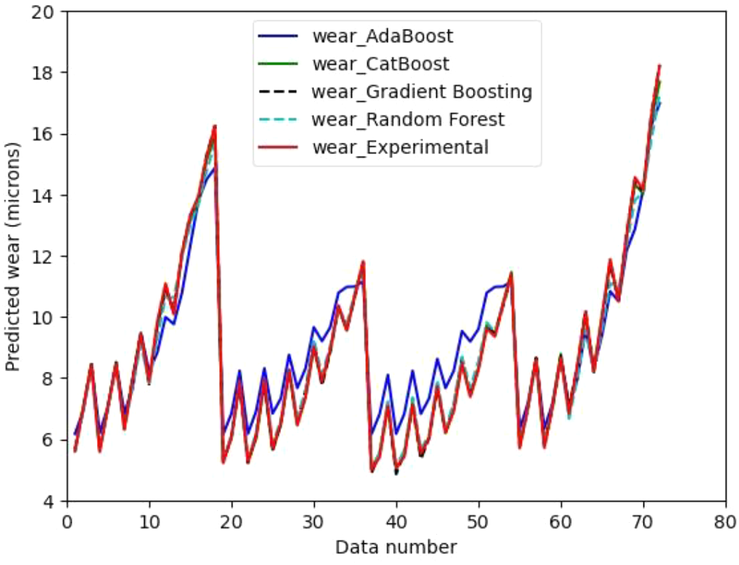
Fig. 6: Predicted wears versus Data number

In comparison to other models, the Gradient Boosting model exhibits lower MAE, RMSE, and AAD% values. This model makes use of gradient descent for identifying the problems with the past predictions made by the learners. The previous error is brought to light and as weaker learners are added to the next learner, the error is gradually decreased.

In comparison to other models, the AdaBoost model exhibits MAE, RMSE, and AAD% of higher values. Because of presence of noisy data and outliers, this model is sensitive. Performance of this model also depends upon class distribution of the dataset. AdaBoost model may not function effectively if the weak learners are complicated, which could lead to unstable models.

Present study found various limitations in the experiments as well as the model, which are given below:

(i)   The actual oral condition is dynamic and complex. A tribometer of Pin-on-disc type was employed in current investigation, is not an exact replica of the oral conditions.

(ii)  Temperature effect on wear was not taken into consideration in this study.

(iii) The wear test was performed at uniform sliding speed, but it can be conducted at various sliding speeds for studying the wear characteristics of composites.

(iv)  Wear prediction accuracy using ML models can be improved by increasing the sample size.

5  CONCLUSIONS

In this work four different ML algorithms were applied for wear prediction of dental composites immersed in a chewable tobacco condition prior to the test. AdaBoost, CatBoost, Gradient Boosting and Random forest models predicted an MAE of 0.7111, 0.0773, 0.0771 and 0.8020 respectively, and R2 of 0.9207, 0.9985, 0.9989 and 0.9899 respectively. CatBoost, Gradient Boosting and Random forest models outperformed the AdaBoost model with superior accuracy. It has been found that number of days of immersion’ is the main significant feature which can affect the ‘wear’. Machine learning is found to be an efficient analytical method having potential to predict wear of dental materials based on limited data set.

References

1. J.A. Arsecularatne, N.R. Chung and M. Hoffman. (2016). Biosurf. Biotribol. 2(3) 102. [Google Scholar]

2. H.K. Shobha, M. Sankarapandian, S. Kalachandra, D.F. Taylor, J.E. McGrath. (1997). J. Mater. Sci. Mater. Med. 8(6) 385. [Google Scholar]

3. A. Peutzfeldt. (1997). Eur. J. Oral Sci. 105(2) 97. [Google Scholar]

4. I. Sideridou, V. Tserki and G. Papanastasiou. (2002). Biomat. 23(8) 1819. [Google Scholar]

5. E.C. Yilmaz. (2020). Mater.Technol. 35(3) 159. [Google Scholar]

6. E.C. Yilmaz and R. Sadeler. (2018). Mech. Compos. Mater. 54(3) (2018) 395. [Google Scholar]

7. E.Ç. Yilmaz and R. Sadeler. (2021). J.Bio-Tribo-Corros. 7: 91. [Google Scholar]

8. E.Ç. Yilmaz and R. Sadeler. (2018). J. Dent.Res. Rev. 5(4) 111. [Google Scholar]

9. E.Ç. Yilmaz. (2020). Mech.Compos.Mater. 56: 261. [Google Scholar]

10. E.Ç. Yilmaz. (2019). Mater. Technol. 34(11) 645. [Google Scholar]

11. M. Giannini, M. Di Francescantonio, R. R. Pacheco, L.C. CidreiraBoaro and R.R. Braga. (2014). Oper. Dent. 39(3) 264. [Google Scholar]

12. A. Suryawanshi and N. Behera. (2022). Mater. Sci. Technol. 53(5) 617. [Google Scholar]

13. R.V. Mesquita, J. Geis-Gerstorfer. (2008). Dent. Mater. 24(5) 623. [Google Scholar]

14. E.C. Yilmaz. (2020). Mater.Technol. 35(3) 159. [Google Scholar]

15. M. Pantic, A. Dordevic, M. Eric, S. Mitrovic, M. Babic, D. Dzunic and M. Stefanovic. (2018). Tribol. Ind. 40(4) 692. [Google Scholar]

16. A.S. Suryawanshi, N. Behera. (2023). Comput. Methods Biomech. Biomed. 26(6) 710. [Google Scholar]

17. O. Altay, T. Gurgenc, M. Ulas and C. Özel. (2020). Friction 8: 107. [Google Scholar]

18. M.E. Machoy, L. Szyszka-Sommerfeld, A. Vegh, T. Gedrangea and K. WoŸniak. (2020). Adv. Clin. Exp. Med. 29(3) 375. [Google Scholar]

19. M.L. Sun, Y. Liu, G.M. Liu, D. Cui, A.A. Heidari, W.Y. Jia, X. Ji, H.L. Chen, Y.G. Luo. (2020). IEEE Access 8: 184360. [Google Scholar]

20. M.T. Alharbi, M. M. Almutiq. (2022). J. Healthc. Eng., 1. [Google Scholar]

21. H.W. Elani, A. Batista, W.M. Thomson, I. Kawachi and A. Chiavegatto Filho. (2021). PloS one 16(6) e0252873. [Google Scholar]

22. S. Patil, S. Albogami, J. Hosmani, S. Mujoo, M.A. Kamil, M.A. Mansour, H.N. Abdul, S. Bhandi and S.S.S.J. Ahmed. (2022). Diagnostics 12: 1029. [Google Scholar]

23. A. A. Haidan, O. Abu-Hammad and N. Dar-odeh. (2014). Comput. Math.Methods Med. 2014: 1. [Google Scholar]

24. Q. Yang, L. Zhenzhe, Y. Zhaojing, L. Haotian, H. Xiangya and G. Lisha. (2022). J. Dent. 118 : 103947. [Google Scholar]

25. Y. Wenzhe, H. Aimin, L. Shuai, W. Yong, X. Bin. (2020). BMC Oral Health 20: 141. [Google Scholar]

26. F. Carrillo-Perez, O.E. Pecho, J.C. Morales, R.D. Paravina, A.D. Bona, R. Ghinea, R. Pulgar, M. Perez and L.J. Herrena. (2020). J. Esthet. Restor. Dent. 34(1) 259. [Google Scholar]

27. N. Nuraliza, S. Syahrullail and M. Faizal. (2016). Jurnal Tribologi. 9: 45. [Google Scholar]

28. A. Suryawanshi and N. Behera. (2020). Proc. Int. Conf. Intelligent Manufacturing and Automation, Singapore. [Google Scholar]

29. D.J. Callaghan, A. Vaziri and H. Nayeb-Hashemi. (2006). Dent. Mater. 22(1) 84. [Google Scholar]

30. E. Sajewicz. (2009). Tribol.Int. 42(2) 327. [Google Scholar]

31. A. Suryawanshi and N. Behera. (2020). Proc. Inst. Mech. Eng. Part H. 234(10) 1106. [Google Scholar]

32. A. Suryawanshi and N. Behera. (2021). Jurnal Tribologi 29: 84. [Google Scholar]

33. S. Shalev-Shwartz and S. Ben-Davi. (2014). Cambridge University Press. [Google Scholar]

34. V. Vapnik. (1992). Adv. Neural Inf. Process Syst. 831. [Google Scholar]

35. H. Zhang, M. Cisse, Y.N. Dauphin, D. Lopez-Paz. (2018). 6thInt. Conf. on learning representations. [Google Scholar]

36. Singer G, Marudi M. (2020). Entropy 22(8) 871. [Google Scholar]

37. Y. Freund, R. Schapire and N. Abe. (1999). Trans. Jpn. Soc. Artif.Intell. 14: 1612. [Google Scholar]

38. A.V. Dorogush, V. Ershov and A. Gulin. (2018). arXiv preprint arXiv, 1810.11363. [Google Scholar]

39. L. Prokhorenkova, G. Gusev, A. Vorobev, A.V. Dorogush and A. Gulin. (2018). Adv. Neural Inf. Process Syst. 31. [Google Scholar]

40. G.M. Huang, L.F. Wu, X. Ma, W.Q. Zhang, J.L. Fan, X. Yu, W.Z. Zeng and H.M. Zhou. (2019). J. Hydrol. 574: 1029. [Google Scholar]

41. H. Rao, X. Shi, A.K. Rodrigue, J. Feng, Y. Xia, M. Elhoseny, X. Yua and L. Gu. (2019). Appl. Soft Comput. 74: 634. [Google Scholar]

42. Y. Chang, J. Lin, J. Shieh and M. Abbod. (2012). Adv. Fuzzy Syst. 2012: 9. [Google Scholar]

43. E. Maleki. (2015). IOP Conf. Ser. : Mater. Sci. Eng. 103. [Google Scholar]