DOI:10.32604/jbd.2022.028078
| Journal on Big Data DOI:10.32604/jbd.2022.028078 | |
| Article |
A Noise Extraction Method for Cryo-EM Single-Particle Denoising
1Key Laboratory of Intelligent Computing Information Processing, Ministry of Education, School of Computer Science and School of Cyberspace Science, Xiangtan University, Xiangtan, 411100, China
2Department of Computer Science, The University of Georgia, Georgia, 30301, USA
*Corresponding Author: Jianquan Ouyang. Email: oyjq@xtu.edu.cn
Received: 04 March 2022; Accepted: 05 April 2022
Abstract: Cryo-Electron Microscopy (cryo-EM) has become a powerful method to study the structure and function of biological macromolecules. However, in clustering tasks based on the projection angle of particles in cryo-EM, the noise considerably affects the clustering results. Existing denoising algorithms are ineffective due to the extremely low signal-to-noise ratio (SNR) of cryo-EM images and the complexity of noise types. The noise of a single particle greatly influences the orientation estimation of the subsequent clustering task, and the result of the clustering task directly affects the accuracy of the 3D reconstruction. In this paper, we propose a construction method of cryo-EM denoising dataset that uses U-Net to extract noise blocks from cryo-EM images, superimpose the noise block with the projected pure particles to construct our simulated dataset. Then we adopt a supervised generative adversarial network (GAN) with perceptual loss to train on our simulated dataset and denoise the real cryo-EM single particle. The method can solve the problem of poor denoising performance caused by assuming that the noise of the Gaussian distribution does not conform to the noise distribution of cryo-EM, and it can retain the useful information of particles to a great extent. We compared traditional image filtering methods and the classic deep learning denoising algorithm DnCNN on the simulated and real datasets. Experiment results show that the method based on deep learning has more advantages than traditional image denoising methods. It is worth mentioning that our method achieves a competitive peak signal to noise ratio (PSNR) and structural similarity (SSIM). Moreover, visualization results, indicate that our method can retain the structure information and orientation information of particles to a greater extent compared with other state-of-the-art image denoising methods. It means that our denoising task can provide considerable help for subsequent cryo-EM clustering tasks.
Keywords: Cryo-EM; noise extraction; denoising; GAN
With the development of science and technology, researchers have discovered that visualization of the structure of biological macromolecules is essential for studying the functional properties and molecular mechanisms of biological macromolecules. However, because clear images of biological macromolecules cannot be obtained, the structure of many biological macromolecules cannot be accurately determined. The methods currently used for the analysis of the 3D structure of biological macromolecules are rough as follows: Cryo-Electron Microscopy, cryo-EM [1]; X-ray crystallography, X-ray [2]; Nuclear Magnetic Resonance, NMR [3]. Given that Cryo-EM 3D reconstruction only requires a small number of high-purity samples, a small concentration can reconstruct biological macromolecules well [4]. Therefore, many researchers have begun to pay attention to cryo-EM technology.
The main idea of cryo-EM technology is to cool the biological macromolecules quickly, observe the sample with a transmission electron microscope at a low temperature, and obtain the 3D structure of the sample through image processing and reconstruction calculation.
Image quality plays a crucial role in the 3D reconstruction of cryo-EM. In the process of irradiating biological macromolecules with a projection electron microscope, the intensity of the electron beam is usually reduced to protect the functional structure of the biological macromolecules. However, this will also result in a low SNR of cryo-EM images obtained in this way [5]. Cryo-EM particle selection are often based on automatic or semi-automatic particle selection software such as Relion [6], Spider [7], EMAN2 [8], XMIPP [9], and CryoSPARC [10]. Most of these methods are based on template matching, edge detection, image segmentation, etc. The single-particles selected by these methods still have a lot of noise, and the SNR is extremely low. However, low SNR of single-particle images equates to a large error in estimating the particle orientation by using the equivalent line phase residual evaluation method and a poor clustering result. The clustering result has a considerable impact on the subsequent 3D reconstruction. Therefore, establishing an effective cryo-EM single-particle denoising method that can effectively improve the clustering results and the accuracy of 3D reconstruction.
For the denoising problem of cryo-EM images, several existing cryo-EM image filtering techniques, such as bilateral filters, Gaussian filters, and transform-domain methods BM3D and KSVD, lose large amounts of particle edge information and internal detail information under an extremely low SNR of cryo-EM images and cannot achieve good results [11]. Current deep-learning based methods aim to minimize the mean-squared error (MSE) [12] between noisy and clean particle images. Although this approach can improve the peak SNR (PSNR) [13], it loses the important structural details of the particles. Moreover, the denoising method based on deep learning needs to use paired datasets to train the noise network and implicitly learn the rules of noise. Therefore, reasonable dataset construction is important for deep learning algorithms. However, finding a suitable cryo-EM dataset is difficult. Generally, there are only noise-containing single-particle images after single-particle selection of cryo-EM original images without corresponding clean images, or there are high-definition particle images obtained by projecting the 3D reconstructed model without the corresponding noisy particles. Therefore, training the denoising network to learn the mapping of similar noise from clean images to real noisy images is difficult.
Unlike in natural image denoising, the light field distribution of a natural image caused by direct and scattered light can be considered uniform, and the noise generated by the image sensor is mostly Gaussian noise [14]. Therefore, in the task of blind denoising of natural images using deep learning algorithms, many scholars use Gaussian noise to simulate the noise in natural images. However, this method is challenging to achieve good results for actual image denoising with complex noise types [15]. Because of the difference between cryo-EM and natural image imaging principles, different types of image noises are generated during the acquisition, storage, and signal conversion of cryo-EM images. The types of cryo-EM noise, such as ice crystal particles, noise caused by noise itself, machine vibration during operation, and changes in the magnetic field in the experimental environment, are complicated. Analyses of cryo-EM images have found that the common noise types of cryo-EM images include Gaussian noise, Poisson noise [16], gamma noise [17], and Rayleigh noise [18]. These difficulties pose challenges to the denoising of cryo-EM images. At present, some scholars use the construction method of natural image denoising paired dataset for the construction of paired dataset for cryo-EM single-particle denoising task, that is to add Gaussian noise with fixed signal-to-noise ratio to clean particles. However, using this method to build the dataset exhibits a major drawback because the original noise distribution of cryo-EM images is much more complex than that of Gaussian noise [14]. This condition means that Gaussian noise cannot simulate the noise of real cryo-EM images well. Achieving good results in real cryo-EM image denoising is difficult.
To solve these problems, we propose a noise extraction algorithm for cryo-EM images. It uses U-Net [19] to segment the original cryo-EM images, extracts the noise block, builds a paired dataset, and uses an improved GAN to denoise the cryo-EM single-particle images. The main contributions of this paper are as follows:
(1) To solve the difficulty of constructing a paired dataset in the cryo-EM image denoising task, we propose a noise extraction algorithm for cryo-EM images. This algorithm uses U-Net to segment the original cryo-EM images into three categories: noise, pollution, and particles. Then, the noise area is extracted to form a noise block corresponding to the clean particles, thereby constructing a paired dataset.
(2) To solve the problem that conventional deep learning methods tend to lose particle details in cryo-EM images with low SNR. This paper adopts GAN with perceptual loss and adds conditional constraints to generate denoising images. The method we use can reduce the noise level of cryo-EM single-particle images and retain the particle details and direction information to a large extent.
2.1 Denoising Algorithm of Cryo-EM Images
The algorithms for cryo-EM image denoising in practical applications are mainly divided into the following categories.
(1) The first category covers algorithms that work in the spatial domain. These methods usually use different image smoothing templates to perform image convolution. Local and non-local filtering are methods that work in the spatial domain. Wei et al. [20] designed an adaptive non-local filter that uses a wide range of pixels to estimate the pixel value after denoising. Wang et al. [21] proposed a filtering method based on non-local means that uses the rotational symmetry of several biomolecules.
(2) The second category encompasses algorithms that use the transform domain. Xian et al. [22] utilized transform-domain filtering methods to solve the noise reduction problem in cryo-EM. However, these methods do not work properly under extremely low SNRs. In addition, Bhamre et al. [23] proposed covariance wiener filtering (CWF) for image denoising and demonstrated that CWF, despite its strong noise reduction effect, requires many data samples to estimate the covariance matrix correctly.
(3) The third category, hybrid domain filtering, refers to algorithms that combine the two aforementioned types. BM3D [24] is the most representative among these algorithms. The BM3D algorithm, which is based on the image before obtaining noise, estimates by transforming similar blocks through cooperative filtering. It is widely compared in experiments due to its good performance. Denoising algorithms that work in the transform domain of the image generally consume long computational time. They require extensive computational resources and cannot remove noise effectively. The denoising effect also decreases rapidly when faced with complex noise.
(4) Owing to the rapid development of deep learning, researchers have also discovered the potential of using deep learning in image denoising. Algorithms based on deep learning can be considered the fourth category. Autoencoders, convolutional neural networks, and other approaches have achieved good results in denoising research. Goodfellow et al. [25] (2014) proposed a GAN for evaluating generative models through an adversarial process. Ledig et al. [26] proposed the SRGAN model, which takes an original high-resolution image, samples it, then tries to restore the image by using a GAN model, thus achieving a natural and close approximation of the original image.
Given the extremely low SNR of cryo-EM images, distinguishing between noise and particles is difficult, which makes traditional methods ineffective for denoising cryo-EM images. The advantages exhibited by deep learning techniques in image processing, indicate that it is possible to process cryo-EM images. Ian J. Goodfellow et al. proposed GAN, which uses the idea of game theory to train two network models against each other. In the original GAN, the network model usually consists of a generative model and a discriminative model. The generator deceives the discriminator by capturing the potential distribution of the real data samples and generating data similar to the real data. The discriminator is a two-classifier, and its task is to do its best to distinguish whether the input is real data or samples generated by the generator. The structures of the generator and discriminator can adopt the currently popular deep neural network. We use a differentiable function G to represent the generator and D to represent the discriminator. G and D continue to improve their generation and discrimination capabilities through confrontation and finally reach a kind of Nash equilibrium. The loss function is shown in Eq. (1), where x is sampled from the real data distribution
In general, for GAN learning, we need to train D to maximize the accuracy of discriminating whether the data comes from real data x or pseudo data
Ledig et al. [26] used GAN in the image super-resolution and achieved good results. SRGAN showed better visual similarity in texture compared with the SRCNN method. Then Yang et al. [27] applied GAN to medical CT image denoising and also achieved good results. Although using MSE [12] can obtain a high PSNR [13], it makes the image lack high-frequency information, and the image texture becomes excessively smooth. We should make the reconstructed high-resolution and real images close in terms of pixel value, high-level overall characteristics, and overall style. Therefore, the authors of SRGAN designed a loss function that assesses a solution with respect to perceptually relevant characteristics. The perceptual loss function (See Eq. (2)) is defined as the weighted sum of a content loss (
Perceptual loss:
The first part is a content-based cost function, and the second part is an adversarial learning-based cost function. The content-based cost function not only minimizes the MSE [12] of the pixel space, but also includes an MSE [12] based on the feature space, which is a high-level feature of the image extracted by the VGG network.
Content loss:
The authors define VGG loss based on the ReLU activation layers of the pre-trained 19-layer VGG network described in Simonyan et al. [28].
Adversarial loss:
In addition to the content losses described so far, the generative component of our GAN is added to perceptual loss. Generative loss
3.1 Construction of Cryo-EM Single-Particle Denoising Task Paired Dataset
Since the real cryo-EM single-particle image has no corresponding clean particle image, we can regard the cryo-EM single-particle denoising task as an image blind denoising problem. The image blind denoising problem is to remove unknown noise from noisy images. The previous image denoising methods rely on image prior knowledge modeling to solve the problem of image blind denoising. However, most of the image prior knowledge used in these methods is defined based on human knowledge, and it is difficult to obtain all the features of the image, these methods only the internal information of the input image is used without any external information, so it lacks generality. Deep learning-based methods such as DnCNN have achieved state-of-the-art denoising effects on image non-blind denoising problems. Still, they are not suitable for image blind denoising problems, mainly because deep learning algorithms use paired datasets to train a deep denoising network and implicitly learn the underlying noise distribution. Therefore, for denoising problems with known noise distribution (such as Gaussian noise), a paired dataset can be constructed by adding Gaussian noise and trained with a deep convolutional network for denoising. However, such datasets are difficult to obtain in reality, or the noise distribution is difficult to derive. Generally speaking, we can only obtain noise images with unknown noise information. In real life, the noise distribution of these unknown noise images may be more complicated, so, using existing models trained on a specific noise, such as Gaussian noise, does not give good results [15].
For the blind denoising problem of cryo-EM images, the current deep-learning based method adds Gaussian noise with different noise levels to the clean particles of cryo-EM projection; this is a common method for deep learning to solve the problem of unpaired datasets for denoising tasks. The reason why Gaussian noise is used for analog noise is that in natural images, the light field distribution of natural images caused by direct light and scattered light can be considered to be uniform, and the noise generated by the sensor inside the camera is primarily Gaussian noise so that it can be approximated as Gaussian noise. However, since cryo-EM will generate different types of image noises during acquisition, storage, and signal conversion, such as Gaussian noise, Poisson noise, Rayleigh noise, etc. Therefore, the method of adding Gaussian noise cannot effectively simulate the complex noise distribution of cryo-EM images. This method limits the capability for noise modeling and further affects the denoising performance, and the denoising effect of cryo-EM images with low SNR and complex noise distribution is poor. Therefore, it may be difficult to achieve good results when this method is applied to the image blind denoising problem of cryo-EM. This problem would be solved if abundant external information on cryo-EM images is given. In 2018, Jingwen Chen et al. [15] proposed a noise modeling method based on generative adversarial networks for the blind denoising problem of unknown noise images, which proposed a novel two-step framework, firstly extracting noise blocks. Then the extracted noise blocks are input into the generative adversarial network, the noise distribution is simulated, and the noise is modeled, thereby constructing a suitable paired dataset. The performance is better than the method of directly constructing a paired dataset by Gaussian noise on the high-definition dataset for training.
This paper proposes a noise extraction algorithm for cryo-EM images. The algorithm segments the original cryo-EM image through U-Net. Then, the cryo-EM image’s pure noise block is extracted to construct a cryo-EM single-particle paired dataset of the denoising task. Section 3.1.1 describes the specific process of using U-Net to segment the original cryo-EM image. Section 3.1.2 presents the specific process of extracting pure noise blocks of cryo-EM images.
3.1.1 U-Net Segmentation of the Original Cryo-EM Image
In the noise modeling method proposed by Chen et al. [15] for the blind denoising problem of unknown noise images, noise extraction is to extract noise blocks from the part with a relatively weak background in a given noise image, and the basic approach is to assume that the mean of the same type of noise is 0, and an approximate noise patch is obtained by subtracting the mean of the relatively smooth patches in the noisy image.
The noise and information of natural images are often closely connected. The areas containing noise usually contain useful background information or object information. Therefore, the noise extraction of natural images may be more effective from weak background modules. However, the noise and information distribution of cryo-EM and natural images are different. The particularity of the cryo-EM image is that its noise area and useful particle area do not completely overlap. Many regions that do not contain particle information contain pure noise blocks. Therefore, we can consider segmenting the original cryo-EM image to extract pure noise blocks. We use U-Net, segment the original cryo-EM image and classify the original cryo-EM image into three categories: pure noise, noise mixed with pollution, and particles.
To achieve the above-method, we label and classify the original images of cryo-EM. We divide the targets into three categories, namely, background noise, pollution, and particles. Pollution here refers to ice pollution, impurities, and carbon-rich areas. When selecting particles, we do not select particles that are heavily polluted. We mark the particles at the point level, so they are only associated with a few surrounding pixels. We use pixel-level annotations for large areas such as pollution. The remaining unlabeled pixels are automatically classified as background noise. Fig. 1 shows the labeling of an 80S ribosome (EMPIAR-10153) cryo-EM image.

Figure 1: (a) Original cryo-EM image of the 80 s ribosome; (b) Label image of (a). In which the blue area represents background noise, the red area represents pollution, and the green dot is the particle label
The U-Net image segmentation algorithm can segment background noise, pollution, and particles from noisy images without excessive training images. It calculates the softmax score vector of each pixel through function calculations and selects each pixel. The category with the highest score is used as the predicted category of the pixel value. Then, the category label of each pixel value is obtained. The pixel label of the background noise category is 0, the pixel label of the pollution category is 1, and the pixel label of the particle category is 2.
3.1.2 Noise Block Extraction of the Original Cryo-EM Image
After using the U-Net image segmentation algorithm, we input a cryo-EM original image and obtain a pixel label matrix.
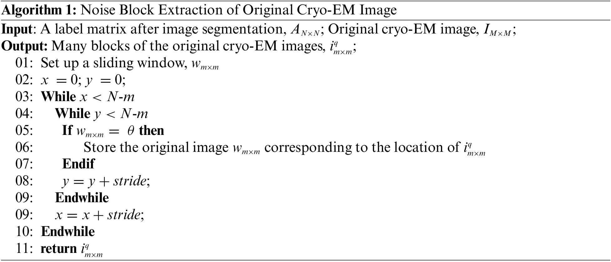
Fig. 2 describes the overall paired dataset construction process for the cryo-EM single-particle noise reduction task.
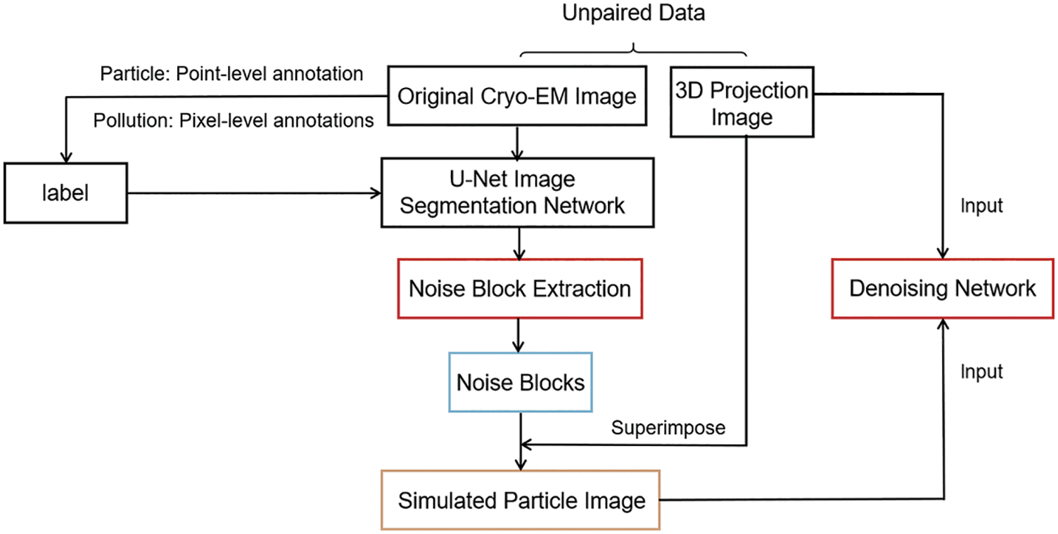
Figure 2: Process of building the paired dataset for the cryo-EM single-particle denoising task
Fig. 3 shows the simulated cryo-EM single-particle image with Gaussian noise and the method used in this paper, as well as the real cryo-EM single-particle image. (Real cryo-EM single particle image (d) do not match simulated images.
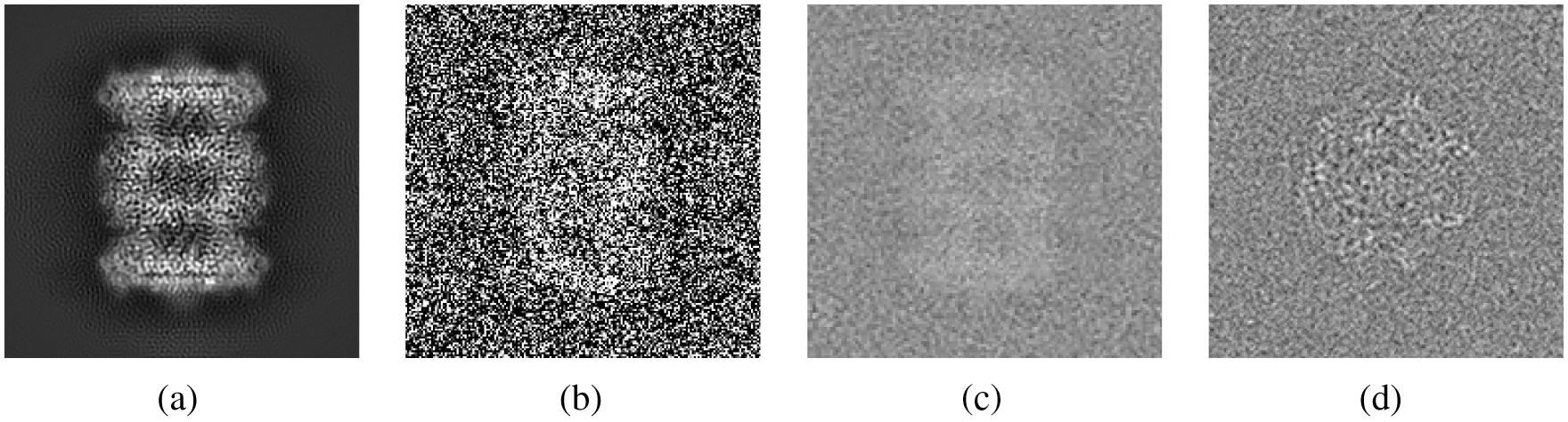
Figure 3: (a) Clean particle image after projection by cryo-EM; (b) cryo-EM single-particle image simulated by Gaussian noise method; (c) cryo-EM single-particle simulated by our method; (d) Real cryo-EM single-particle image
3.2 Denoising Network: GAN with Perceptual Loss
Traditional image filtering technology cannot function normally when processing cryo-EM images with extremely low SNR and low contrast. Related algorithms greatly lose the details and contour information of the particles. Although the denoising method based on deep learning has achieved good results in image denoising, the mean square error of using MSE [12] will make the denoised image become too smooth and lose the detailed texture information. However, in particle denoising tasks, the structure and orientation information of particles greatly influence the results of subsequent clustering tasks. Therefore, we need to establish a denoising method that effectively removes noise and retains particle information. To solve these problems, we apply GAN with perceptual loss to the cryo-EM single-particle image denoising task and combine the improvement ideas of GAN to enhance the cryo-EM denoising task. The GAN with perceptual loss can retain the detailed information of the particles to the greatest extent, and GAN, which is robust to various noises, learns the implicit characteristics of noise. GAN focuses on the migration of data noise from strong statistics to weak statistics. Hence, it has strong adaptability to noise and blur and increases the processing effect on low-SNR cryo-EM images.
The goal of the generator network is to generate pure particle images through generators. The discriminator continuously improves its resolving power by learning the feature distribution of the 3D projected high-definition particle image. Hence, the generator must generate enhanced-quality particle images to fool the discriminator.
For the network structure, we refer to the design of Alsaiari et al. [29]. We use the residual connection in the structure of the generator network. The network is divided into three blocks, convolution layers, residual blocks, and deconvolution layers. The convolution layers contains convolution, BN, and LReLU. In the residual blocks, the same structure as the convolutional layer is used, the difference is that a shortcut connection is used to implement the residual structure, which makes the network efficient and achieve good convergence during training. The input of the generator network is the simulated particle image previously constructed; the output of the generator network is the particle image after denoising; The size of the input and output images are (256, 256). We use five convolutional networks with batch normalization and the LReLU activation function for the discriminator network. The input of the discriminator network is the denoising particle image generated by the generator and the corresponding clean particle image. Figs. 4 and 5 show diagrams of the generator and discriminator network structures, respectively.
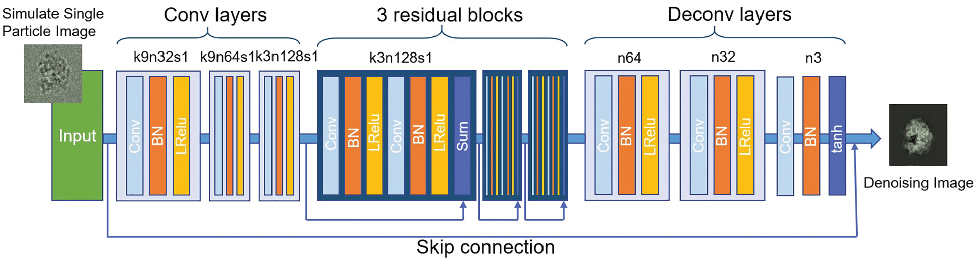
Figure 4: Generator networks
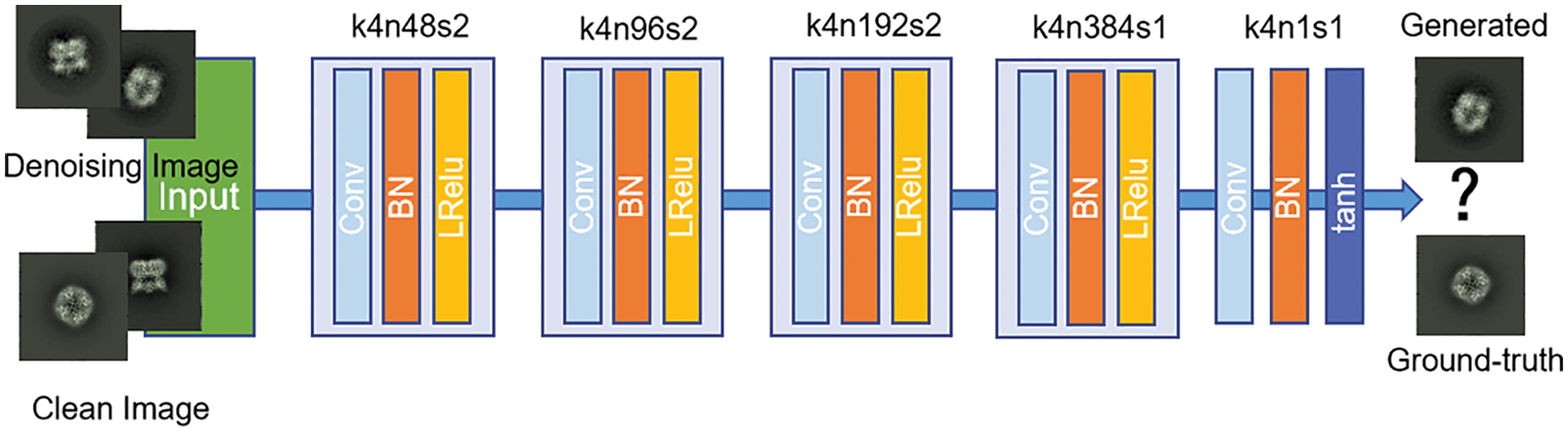
Figure 5: Discriminator networks
GAN was traditionally used for unsupervised learning tasks. The unsupervised training method adds a random noise z to the generator to generate images. However, this method is challenging when used to control the output image. That is, we cannot decide which random noise to use to produce the image we want unless we try all the initial distributions. Given that we have constructed a paired dataset of cryo-EM images, we can use the idea of image-to-image translation [30] to solve it and change the unsupervised training method of GAN to supervised. Image-to-image translation [30] is the process of obtaining the desired output image based on an input image. It can be regarded as a mapping between an image and another image. For the cryo-EM image denoising task, we use x to represent the simulated noisy particle image.
To ensure similarity between the input and output image, we use
To preserve the structure information of the particles to the greatest extent during training, we adopt perceptual loss, which we call
Therefore, the overall loss function is defined in Eq. (8).
The source of our experimental dataset is the PDB’s Electron Microscope Database (EMDB) [31]. To improve the generalization of the network, we select various PDB molecules for 3D projection to obtain our clean particle images and selected the corresponding original image for noise block extraction to simulate real noisy particles. The image format obtained from EMDB is mrc and cannot be directly inputted to the neural network. We preprocess the mrc images and convert them to jpg format. Section 4.1, compares the performance of various denoising methods for different noises and different particles in our simulated dataset. Section 4.2, compares the denoising effect of our network on the real particle image when training on the dataset under Gaussian noise and training on the simulated dataset. We also compare the denoising effects of other denoising methods on real particles. Given that real particles do not have corresponding clean particles, the denoising results of real particles can only be evaluated by subjective evaluation.
4.1 Denoising Performance in the Simulation Dataset
We conduct a comparative experiment on the paired dataset we constructed. The experiment compares two indicators, PSNR [13] and SSIM [13], which are two indicators commonly used in the field of image denoising. PSNR is an error-sensitive image quality evaluation index. Generally speaking, the higher the PSNR, the better the quality of denoising. However, this index tends to ignore the visual characteristics, and it often appears inconsistent with the subjective evaluation. SSIM is an index that measures image similarity from the three aspects of image brightness, contrast, and structure. In this experiment, we used simulated images of various particles for training and used the EMD-0406 dataset and EMD-23579 for testing. We added noise blocks of different noise levels to these two particles. Among them, the noise level added to the EMD-0406 dataset is lower, and the noise level added to EMD-23579 is higher. Compare our method with the general filter, the hybrid domain BM3D algorithm, and the deep learning-based DnCNN algorithm.
The denoised images of the EMD-0406 dataset are shown in Fig. 6, and the denoised images of EMD-are shown in Fig. 7. The results of the evaluation indicators are shown in Tab. 1.
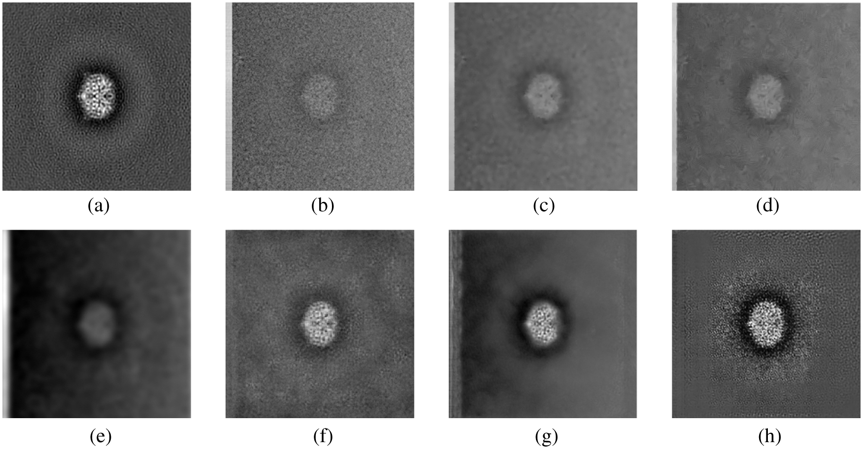
Figure 6: Comparative experiments on the EMD-0406 simulation dataset with a weak noise level: (a) Clean particle image; (b) Noisy image simulated by our method; (c) Bilateral Filters; (d) BM3D; (e) low-pass filter; (f) DnCNN; (g) GAN (Unsupervised); (h) GAN (Ours)
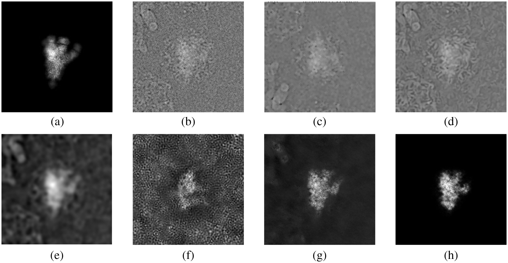
Figure 7: Comparative experiments on the EMD-23579 simulation dataset with a strong noise level: (a) Clean particle image; (b) Noisy image simulated by our method; (c) Bilateral Filters; (d) BM3D; (e) low-pass filter; (f) DnCNN; (g) GAN (Unsupervised); (h) GAN (Ours)
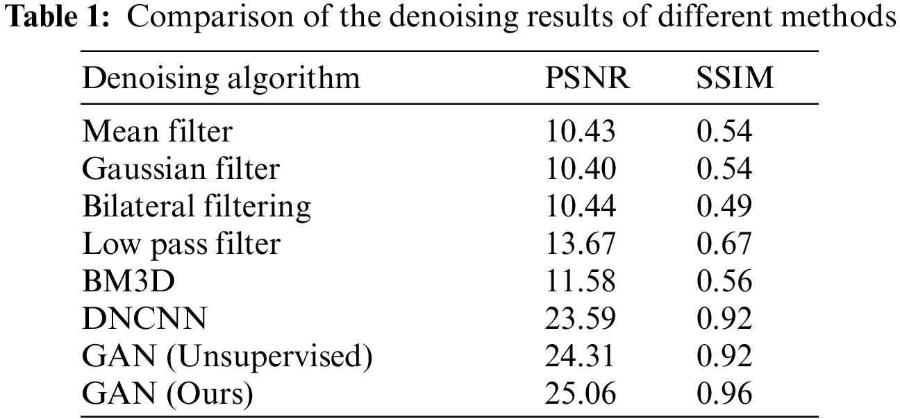
Among the seven compared methods, our method achieves the best PSNR [13] and SSIM [13], and the general filtering method in the spatial domain has the worst results. One of the main reasons is that algorithms in the spatial domain calculate directly based on the pixels of the image; moreover, the signal of cryo-EM images is close to the gray value of noise, so the effect is weak. Compared with the effect in the spatial domain, the effect in the hybrid and transform domains is relatively better. However, the denoising effect we wish to achieve is still not achieved, and the calculation time of these algorithms is long. Compared with these traditional image denoising methods, the denoising algorithm based on deep learning is superior mainly because the deep learning algorithm can learn the rules of noise through the paired dataset we constructed. The GAN-based denoising algorithm can achieve better results than the other deep learning algorithms. The main reason is that GAN pays attention to the migration of data noise from strong statistics to weak statistics and has strong resistance to various noises. It enhances the processing effect on cryo-EM images, which contain complex noise images. In addition, the GAN that we use to join the conditional constraints can learn the features we want, so we obtain the best results.
For the EMD-0406 simulation data denoising experiment with the weak noise level, we show the denoising results of six methods. The visualization results show that the traditional image filtering method is not effective; the methods based on deep learning have shown a great effect and can retain the contours of the particles. However, the approach using DnCNN still retains a certain amount of noise, and the unsupervised GAN-based loses some edge information. Compared with these methods, the method we use can retain the detailed information of the particles to the greatest extent.
For the EMD-23579 simulation data denoising experiment with a strong noise level, we also show the denoising results of six methods. The visualization results reveal that the algorithm based on DnCNN exerts a better effect than the traditional filtering methods. However, it still retains much noise and loses the particles’ structure and orientation information. Compared with DnCNN, GAN has a better denoising effect. Furthermore, compared with the unsupervised training GAN, the method we use can remove noise to the greatest extent and retain the useful information of the particles.
4.2 Denoising Performance in Real Noisy Dataset
In this section, we compared the denoising effect of two methods on real single particle of cryo-EM, one method uses Gaussian noise to train our network, and the other method trains our network with the simulated dataset constructed in this paper. We also compare the denoising images of our method and those of other methods on real particles. The denoising image of the real particle (EMPIAR-10059) is shown in Fig. 8.
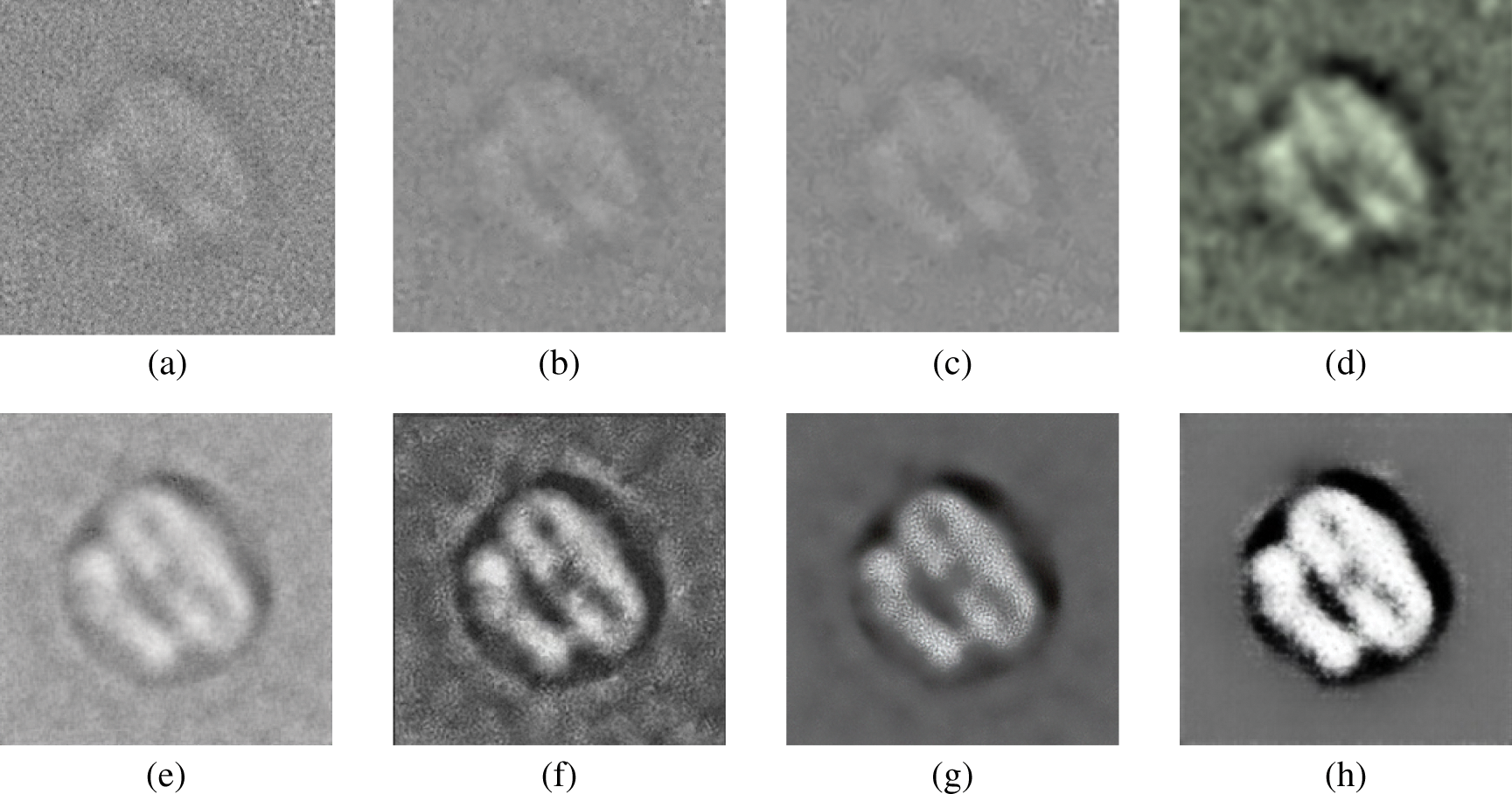
Figure 8: Comparative experiments on the EMPAIR-10059 real dataset : (a) real noisy particle; (b) Bilateral Filters; (c) BM3D; (d) low-pass filter; (e) GAN (ours) trained on Gaussian noise dataset; (f) DnCNN; (g) GAN (Unsupervised); (h) GAN (Ours). (f)-(g) trained with the simulated dataset constructed by our method
The images of the denoising results of real particles show that the traditional filter only has a low-pass filter, which can play a role to a certain extent but still retains a lot of noise. The method based on deep learning has significant effects. Among them, our method has the best effect on retaining the particle’s structure information and orientation information due to the perceptual loss that we added during training. Comparison of (g) and (h) in Fig. 8, both unsupervised GAN (g) and supervised GAN (h) have good denoising effect on real particles, but the supervised GAN we trained can remove noise to a greater extent and retain particle information to a greater extent. It shows that the use of supervised GAN allows the network to better learn the mapping from the input image to the output image, so as to obtain the specified output image. In addition, in Fig. 8, (e) is the denoising effect of our improved GAN network trained by Gaussian noise on real particles. Comparing (e) and subsequent (f), (g), (h), it can be seen that the use of a Gaussian noise training network has a poor denoising effect on real particles. Although the rough outline of the particles can be seen, a large amount of noise is still retained. The method of constructing the dataset using the method in this paper, whether it is DnCNN (f), or unsupervised GAN (g), or supervised GAN (h), the denoising effect is better than (e), which further shows that the dataset constructed with our method is more efficient than using Gaussian noise to build the dataset performs better for cryo-EM single-particle denoising task.
In this paper, we propose a noise extraction algorithm to build a paired dataset and use improved GAN to denoise cryo-EM single-particle images. We provide quantitative indicators and visualization results on simulated datasets and visualization results on real datasets. The experimental results show that our method demonstrates better performance than other state-of-the-art methods, achieves higher PSNR and SSIM, effectively removes particle noise, and retains more useful information. Although the proposed method achieves good performance in PSNR and good visual effects on the retention of particle structure information, for particles that have not been extracted from the noise block of the original cryo-EM image, a large gap still exists between denoised and clean particles. Therefore, in our future work, after extracting enough noise blocks, we will input them into GAN, simulate the distribution, and perform modeling to improve the network’s generalization.
Acknowledgement: We would like to thank the relevant teachers for their help in the experiments, the students in the lab for their contributions, and the National Key Research and Development Project Team for their support in the completion of this article.
Funding Statement: This research has been supported by Key Projects of the Ministry of Science and Technology of the People Republic of China (2018AAA0102301).
Conflicts of Interest: We declare that we have no conflicts of interest to report regarding the present study.
1. M. Adrian, J. Dubochet, J. Lepault and A. W. McDowall, “Cryo-electron microscopy of viruses,” Nature, vol. 308, pp. 32–36, 1984. [Google Scholar]
2. P. Thibault, M. Dierolf, A. Menzel, O. Bunk, C. David et al., “High-resolution scanning x-ray diffraction microscopy,” Science, vol. 321, pp. 379–382, 2008. [Google Scholar]
3. R. K. Harris, “Nuclear magnetic resonance spectroscopy,” Longma n Scien tific & Technical, J. Wiley, Eastern, United States, 1986. [Google Scholar]
4. X. -C. Bai, G. McMullan and S. H. Scheres, “How cryo-EM is revolutionizing structural biology,” Trends in Biochemical Sciences, vol. 40, no. 1, pp. 49–57, 2015. [Google Scholar]
5. H. Lei and Y. Yang, “CDAE: A cascade of denoising autoencoders for noise reduction in the clustering of single-particle cryo-EM images,” Frontiers in Genetics, vol. 11, pp. 1799, 2021. [Google Scholar]
6. J. Zivanov, T. Nakane, B. O. Forsberg, D. Kimanius, W. J. Hagen et al., “New tools for automated high-resolution cryo-EM structure determination in RELION-3,” ELife Sciences, vol. 7, pp. 519–530, 2018. [Google Scholar]
7. J. Frank, M. Radermacher, P. Penczek, J. Zhu, Y. Li et al., “SPIDER and WEB: Processing and visualization of images in 3D electron microscopy and related fields,” Journal of Structural Biology, vol. 116, no. 1, pp. 190–199, 1996. [Google Scholar]
8. G. Tang, L. Peng, P. R. Baldwin, D. S. Mann, W. Jiang et al., “EMAN2: An extensible image processing suite for electron microscopy,” Journal of Structural Biology, vol. 157, no. 1, pp. 38–46, 2007. [Google Scholar]
9. J. De la Rosa-Trevín, J. Otón, R. Marabini, A. Zaldivar, J. Vargas et al., “Xmipp 3.0: An improved software suite for image processing in electron microscopy,” Journal of Structural Biology, vol. 184, no. 2, pp. 321–328, 2013. [Google Scholar]
10. A. Punjani, J. L. Rubinstein, D. J. Fleet and M. A. Brubaker, “CryoSPARC: Algorithms for rapid unsupervised cryo-EM structure determination,” Nature Methods, vol. 14, no. 3, pp. 290–296, 2017. [Google Scholar]
11. J. Ouyang, Y. He, H. Tang and Z. Fu, “Research on DENOISINg of cryo-em images based on deep learning,” Journal of Information Hiding and Privacy Protection, vol. 2, no. 1, pp. 1–9, 2020. [Google Scholar]
12. Z. Wang, A. C. Bovik, H. R. Sheikh and E. P. Simoncelli, “Image quality assessment: From error visibility to structural similarity,” IEEE Transactions on Image Processing, vol. 13, no. 4, pp. 600–612, 2004. [Google Scholar]
13. A. Hore and D. Ziou, “Image quality metrics: PSNR vs. SSIM,” in IEEE Int. Conf. on Pattern Recognition, Istanbul, 2010. [Google Scholar]
14. F. Pascal, Y. Chitour, J. P. Ovarlez, P. Forster and P. Larzabal, “Covariance structure maximum-likelihood estimates in compound Gaussian noise: Existence and algorithm analysis,” IEEE Transactions on Signal Processing, vol. 56, no. 1, pp. 34–48, 2007. [Google Scholar]
15. J. W. Chen, J. W. Chen, H. Y. Chao and M. Yang, “Image blind denoising with generative adversarial network based noise modeling,” in IEEE Conf. on Computer Vision and Pattern Recognition, Los Alamitos, 2018. [Google Scholar]
16. I. Rodrigues, J. Sanches and J. Bioucas-Dias, “Denoising of medical images corrupted by poisson noise,” in IEEE Int. Conf. on Image Processing, California, 2008. [Google Scholar]
17. Y. G. Kondratiev, J. L. da Silva, L. Streit and G. F. Us, “Analysis on poisson and gamma spaces,” Infinite Dimensional Analysis, Quantum Probability and Related Topics, vol. 1, no. 1, pp. 91–117, 1998. [Google Scholar]
18. C. G. Gunther, “Comment on estimate of channel capacity in Rayleigh fading environment,” IEEE Transactions on Vehicular Technology, vol. 45, no. 2, pp. 401–403, 1996. [Google Scholar]
19. O. Ronneberger, P. Fischer and T. Brox, “U-Net: Convolutional networks for biomedical image segmentation,” in Int. Conf. on Medical Image Computing and Computer-Assisted Intervention, Munich, 2015. [Google Scholar]
20. D. Y. Wei and C. C. Yin, “An optimized locally adaptive non-local means denoising filter for cryo-electron microscopy data,” Journal of Structural Biology, vol. 172, no. 3, pp. 211–218, 2010. [Google Scholar]
21. J. Wang and C. Yin, “A Zernike-moment-based non-local denoising filter for cryo-EM images,” Science China Life Sciences, vol. 56, no. 4, pp. 384–390, 2013. [Google Scholar]
22. Y. Xian, H. Gu, W. Wang, X. Huang, Y. Yao et al., “Data-driven tight frame for cryo-em image denoising and conformational classification,” in IEEE Global Conf. on Signal and Information Processing, California, 2018. [Google Scholar]
23. T. Bhamre, T. Zhang and A. Singer, “Denoising and covariance estimation of single particle cryo-EM images,” Journal of Structural Biology, vol. 195, no. 1, pp. 72–81, 2016. [Google Scholar]
24. K. Dabov, A. Foi, V. Katkovnik and K. Egiazarian, “Image denoising by sparse 3-D transform-domain collaborative filtering,” IEEE Transactions on Image Processing, vol. 16, no. 8, pp. 2080–2095, 2007. [Google Scholar]
25. I. Goodfellow, J. Pouget-Abadie, M. Mirza, B. Xu, D. Warde-Farley et al., “Generative adversarial nets,” Advances in Neural Information Processing Systems, vol. 27, pp. 2672–2680, 2014. [Google Scholar]
26. C. Ledig, L. Theis, F. Huszár, J. Caballero, A. Cunningham et al., “Photo-realistic single image super-resolution using a generative adversarial network,” in IEEE Conf. on Computer Vision and Pattern Recognition, Honolulu, 2017. [Google Scholar]
27. Q. Yang, P. Yan, Y. Zhang, H. Yu, Y. Shi et al., “Low-dose CT image denoising using a generative adversarial network with wasserstein distance and perceptual loss,” IEEE Transactions on Medical Imaging, vol. 37, pp. 1348–1357, 2018. [Google Scholar]
28. K. Simonyan and A. Zisserman, “Very deep convolutional networks for large-scale image recognition,” arXiv:1409.1556, 2014. [Google Scholar]
29. A. Alsaiari, R. Rustagi, M. M. Thomas and A. G. Forbes, “Image denoising using a generative adversarial network,” in IEEE 2nd Int. Conf. on Information and Computer Technologies, Long Beach, 2019. [Google Scholar]
30. P. Isola, J. -Y. Zhu, T. Zhou and A. A. Efros, “Image-to-image translation with conditional adversarial networks,” in IEEE Conf. on Computer Vision and Pattern Recognition, Salt Lake City, 2018. [Google Scholar]
31. S. Velankar, G. van Ginkel, Y. Alhroub, G. M. Battle, J. M. Berrisford et al., “PDBe: Improved accessibility of macromolecular structure data from PDB and EMDB,” Nucleic Acids Research, vol. 44, pp. 385–395, 2016. [Google Scholar]
 | This work is licensed under a Creative Commons Attribution 4.0 International License, which permits unrestricted use, distribution, and reproduction in any medium, provided the original work is properly cited. |