Journal on Big Data DOI:10.32604/jbd.2022.026850
Article

Research and Practice of Telecommunication User Rating Method Based on Machine Learning

Qian Tang, Hao Chen and Yifei Wei*

Beijing University of Posts and Telecommunications, Beijing, 100876, China
*Corresponding Author: Yifei Wei. Email: weiyifei@bupt.edu.cn
Received: 12 January 2022; Accepted: 22 February 2022

Abstract: The machine learning model has advantages in multi-category credit rating classification. It can replace discriminant analysis based on statistical methods, greatly helping credit rating reduce human interference and improve rating efficiency. Therefore, we use a variety of machine learning algorithms to study the credit rating of telecom users. This paper conducts data understanding and preprocessing on Operator Telecom user data, and matches the user’s characteristics and tags based on the time sliding window method. In order to deal with the deviation caused by the imbalance of multi-category data, the SMOTE oversampling method is used to balance the data. Using the Removing features with low variance method and packaging method for feature selection, then the basic models are established. The empirical results of the model show that the Random Forest and XGBOOST ensemble models are better than the single models such as Bayes, SVM, KNN, and Decision Tree. The performance of Decision Tree in single models is better. Therefore, Random Forest, XGBOOST and Decision Tree models were selected to debug the hyper parameters to achieve model optimization. Based on the optimized model, the accuracy, recall, precision, confusion matrix and other indicators are evaluated, and it is concluded that low-level recognition is more accurate than high-level recognition and fewer misjudgments. Comparing the evaluation indicators of each level of different models, it is found that the integrated model performs better, indicating that Random Forest and XGBOOST are more suitable for solving the problem of telecommunications user rating. For this reason, this article proposes an implementation plan based on Random Forest and XGBOOST algorithm and model for the problem of telecommunications user rating.

Keywords: Credit rating; model evaluation; random forest; XGBOOST

1  Introduction

With the reorganization of the communications’ industry and the rise of the “Internet +” model, the competition among the three major telecom operators has intensified, and some Internet companies have also joined the market, and the competition has become more intense. In order to strive for user resources, telecom operators have launched a series of package products, but due to the mismatch of the products recommended to users, the phenomenon of users taking the initiative to leave the network and cancel their accounts frequently occurs. In addition, telecom operators mistakenly assessed online users as being off-network, and forced users to dismantle their accounts, which resulted in a loss of user resources. Whether users actively or passively disconnect from the network, they will cause huge losses to telecom operators. Therefore, it is particularly important to analyze and predict the credit rating of telecom users, introduce matching products to customers of different levels, and obtain the off-network probability through credit analysis, so as improving the accuracy of telecommunications operators in identifying off-network customers.

In recent years, machine learning has been widely used in many fields, providing solutions for the research of big data problems. Some effective traditional machine learning methods are used to solve the credit classification problem. Ali et al. [1] studied the application of Naive Bayes, Generative Adversarial Network and Neural Network algorithms in the identification of credit card fraud and legitimate transactions in e-commerce. Saheed et al. [2] studied the use of Naive Bayes, Random Forest and Support Vector Machine supervised machine learning technology to perform CCF detection on imbalanced German credit card data sets. Dai et al. [3] proposed a combined feature selection method to determine the key features in bank credit rating prediction, and applied it to the training of Random Forest, support vector machine and gradient enhancement classification. Chen et al. [4] effectively uses a recurrent neural network to evaluate corporate credit ratings. Kelen et al. [5] focuses on the comparison of the five classification methods using historical loan application data for a Multipurpose Cooperative. Okur et al. [6] uses Lending Club’s data has studied the application of boost Decision Tree Regression algorithm in credit risk prediction. Prusti et al. [7] uses classification algorithms to identify credit card fraud, and proposes a predictive classification model integrated by five independent algorithms. Qiu et al. [8] adopts the dual-channel credit evaluation model of XGBOOST and GBDT to simplify the overall model, speed up the calculation, and optimize the model indicators.

A number of studies have shown that machine learning models are superior in multi-category credit rating classification and can replace discriminant analysis based on statistical methods, greatly helping credit ratings reduce human interference and improve rating efficiency. Therefore, we have studied a variety of machine learning algorithms, analyzed and processed data from multiple dimensions for telecommunication users, and established a credit rating model for telecommunication users based on model characteristics and model integration.

The rest of the paper is organized as follows. Section 2 introduces the time sliding window method of matching features and labels, the imbalanced data processing method based on SMOTE technology, the CART and XGBOOST algorithm and the calculation method of model evaluation. The data set and experimental details used in this article are shown in Section 3. In Section 4, we made a clear analysis of the experimental results. In Section 5, a brief conclusion is made about this paper.

2  Method

2.1 Time Sliding Window Method

Since the credit rating changes with the user’s communication behavior with time, we choose to use a time sliding window for data integration. As shown in Fig. 1, the communication behavior data of the first three months of the month when the label result is located is integrated into a feature set, that is to say, the communication behavior data of June, July, and August are integrated as features and the credit rating of September is recorded as labels. When the feature set integrated from July, August, and September data is given to the model, we can predict the credit rating in October and adjust the business strategy in time based on this result. Therefore, to predict the credit rating of a user, the matching feature does not require all the monthly data, just select the data in the selected time window for integration.

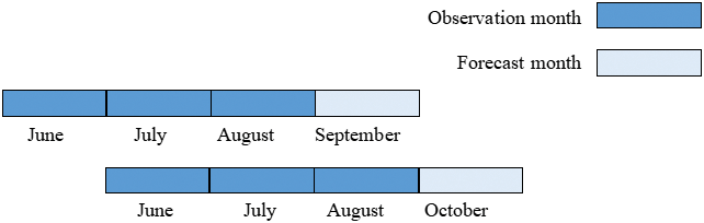
Figure 1: Sliding time window

2.2 Unbalanced Data Processing

In the problem of telecommunications user credit rating prediction, the number of users of each credit rating is counted on a monthly basis, and it is found that the monthly average of the number of users of different levels in a year varies greatly. For minority samples, it is difficult to find the regular patterns in this type of sample. In order to solve this problem, re-sampling is adopted from the data level to balance the number of classes. The SMOTE [9,10] oversampling method is mainly used, which is different from the simple copy sample mechanism of random oversampling. SMOTE synthesizes new samples between two minority samples through linear interpolation, thereby effectively alleviating the over fitting problem caused by random oversampling.

The basic principle of SMOTE is illustrated in Fig. 2 [11,12]. First, select each sample xi in turn from the minority samples as the root sample for the synthesis of the new sample; secondly, according to the up sampling magnification n, randomly select a sample from the k neighbor samples of the same category of xi as the auxiliary sample for the synthesis of the new sample, repeat n times; then perform linear interpolation between the sample xi and each auxiliary sample through Eq. (1), and finally generate n synthesized samples.

xnew,attr=xi,attr+(xj,attr−xi,attr)×γ(1)

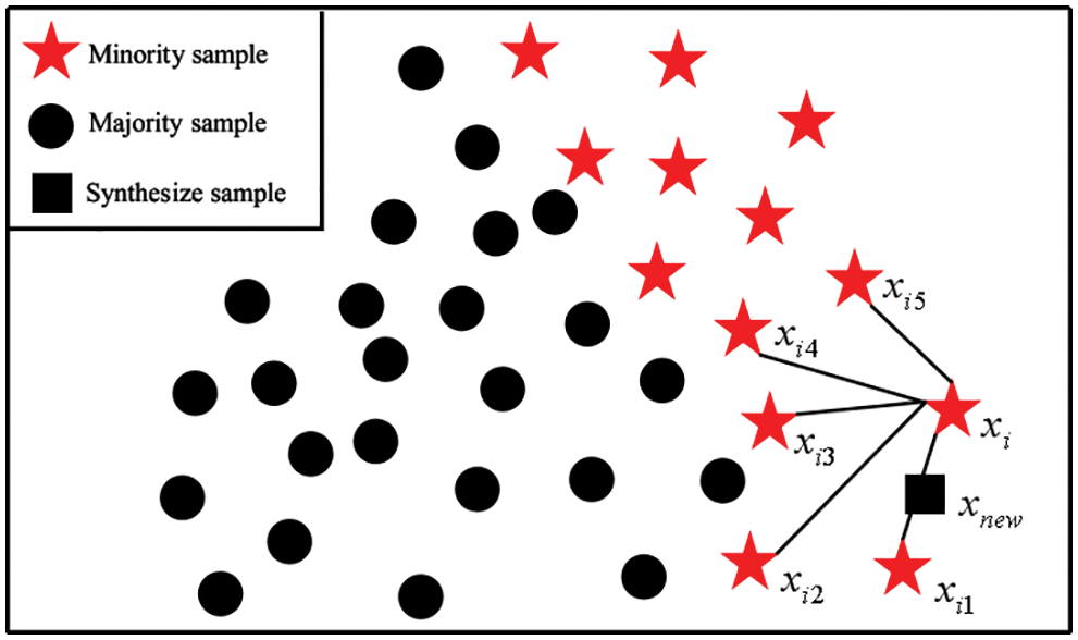
Figure 2: The interpolation illustration of SMOTE algorithm

Among them, xi∈Rd, xi, attr  is the attr attribute value of the i sample in the minority class, attr=1,2,…,d; γ is a random number between [0,1];xij is the j nearest neighbor sample of sample xi, j=1,2,…,k;xnew represents a new sample synthesized between xij and xi. It can be seen from Eq. (1) that the new sample xnew is a sample obtained by interpolation between samples xij and xi.

2.3 Algorithm Implementation

2.3.1 CART

In the classification tree model, the CRAT algorithm uses the GINI coefficient to select the split feature attributes. Assuming there are k credit levels, the probability that the sample point belongs to the k class level is Pk, then the GINI index of the probability distribution is defined as:

Gini(p)=∑k=1Kpk(1−pk)=1−∑k=1Kpk2(2)

Suppose Ck is the sample subset belonging to class k in the telecom user data set D, and the GINI index can be obtained from the Eq. (2):

Gini(D)=1−∑k=1K(|Ck||D|)2(3)

Suppose that condition A divides sample D into two data subsets D1 and D2, then the GINI index of sample D under condition A is:

Gini(D,A)=|D1|DGini(D1)+|D2|DGini(D2)(4)

That is, under condition A, the GINI gain of dividing sample D into two data subsets D1 and D2 is

ΔGini(A)=Gini(D)−Gini(D,A)=(1−∑k=1K(|Ck||D|)2)−(|D1|DGini(D1)+|D2|DGini(D2))(5)

The specific process is as follows:

1)   Calculate the GINI index of the telecommunications data sample D, and then use each feature A in the sample, and each possible value a of A, divide the sample into two parts according to A greater than or equal to a and A less than a, and calculate the Gini(D,A) value;

2)   Find out the optimal segmentation feature and value corresponding to the smallest GINI index Gini(D,A), and judge whether the segmentation stop condition, if not, output the optimal segmentation point;

3)   Recursive call 1) 2);

4)   Generate CART Decision Tree.

2.3.2 XGBOOST

The full name of XGBOOST is Extreme Gradient Boosting [12,13], which can be translated as an extreme gradient boosting algorithm. The principle of the XGBOOST algorithm is to boost the tree model. By combining some tree models together, a stronger classifier is established. The model used in the algorithm is the regression tree model constructed by the CART algorithm. The main implementation step of the XGBOOST algorithm is to continuously add regression trees to the model. Adding a regression tree to it is to learn a new function to fit the residuals of the last prediction. When K trees are obtained, according to the characteristics of the sample, they will fall into the leaf nodes of the corresponding tree. The leaf nodes have corresponding scores. Add the corresponding scores to get the predicted value. The calculation method is as follows:

y^i=ϕ(xi)=∑t=1Kft(xi)(6)

ft(x)=wq(x),w∈RT,q:Rd→{1,2,…,T}(7)

where wq(x) is the score of the leaf node q, and ft is one of the regression trees.

The objective function of the XGBOOST algorithm is defined as:

Obj(Θ)=∑i=1Nl(yi,y^i)+∑j=1tΩ(fj),fj∈F(8)

Ω(ft)=γT+12λ∑j=1Twj2(9)

In order to find ft to minimize the objective function, the objective function is expanded by Taylor series and approximated:

Obj(t)=∑i=1N(l(yi,y^i(t−1))+gift(xi)+12hift2(xi))+Ω(ft)(10)

gi=∂l(yi,y^i(t−1))∂y^i(t−1),hi=∂2l(yi,y^i(t−1))∂2y^i(t−1)(11)

Because the residuals between the predicted scores of the first  t−1 trees and y have no effect on the objective function, the objective function can be optimized as:

Obj(t)=∑i=1N(gift(xi)+12hift2(xi))+Ω(ft)(12)

Define the sample set on each leaf node j as Ij={i∣q(xi)=j}, and the objective function can finally be optimized as:

wj=−GjHj+λ(13)

Obj(t)=−12∑j=1T(Gj2Hj+λ)+γT(14)

Gj=∑i∈Ijgi, Hj=∑i∈Ijhi(15)

Each time a node is split, the gain before and after the split is calculated, and the attribute with the largest gain is selected for splitting. From the previous calculation, the gain can be deduced as:

Gain=12[GL2HL+λ+GR2HR+λ−(GL+GR)2HL+HR+λ]−γ(16)

The larger the Gain value, the more the objective function can be reduced after splitting, and the better.

2.4 Model Evaluation

The classification data in this article is a multi-classification problem, and there is a phenomenon of class imbalance. The accuracy alone will not reflect the quality of the model. Other more widely used indicators are needed for comprehensive measurement. Common indicators are Confusion Matrix, Precision, Recall, F1 measurement, etc. Accuracy is the proportion of samples with correct grade prediction to the total sample. Precision is calculated based on the classification result, among samples classified into a certain grade, the proportion of samples that are actually marked as that grade. Recall is calculated based on the true value of the sample, among the samples that are actually marked as a certain level, the proportion of samples identified as that level. Recall rate and precision rate cannot be achieved at the same time. For comprehensive consideration, their harmonic mean measure F1 is proposed.

F1=2⋅ Precision ⋅ Recall  Precision + Recall (17)

3  Problem Modeling

3.1 Data Description and Processing

The data used in this paper comes from the data of millions of users of a telecom operator in the second half of 2020. Generally, telecommunication user data types are divided into two categories: basic attributes and behavioral data. Let’s understand it in combination with the business. Basic attributes: mainly the customer’s identity information, including the user id of the card, the location of the card and so on. Behavioral data: Mainly data about the customer’s product order, communication behavior, financial behavior, etc., such as, the type of package ordered, call duration, flow, payment amount, arrears, shutdown record, etc.

Combining the telecommunication data and business analysis that can be obtained in practice, the available data is filtered as shown in Tab. 1:

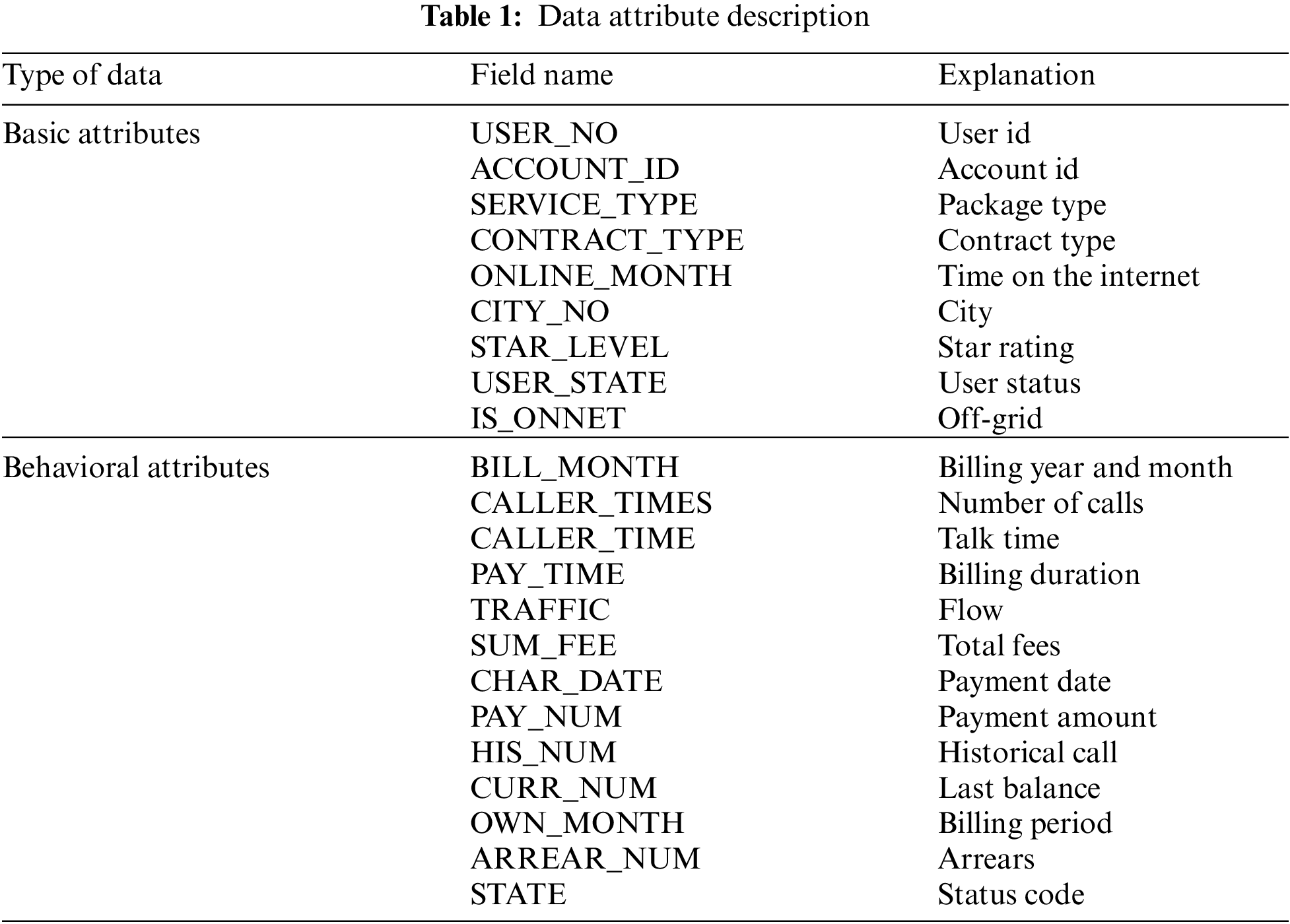
The available million-level telecom user data set is the basic attribute information and communication behavior information data of each user stored in the database. Each attribute of the user is analyzed, and the available data is integrated after selecting useful attributes. The communication behavior occurred in the second half of 2020 in 6 months. According to the time sliding window method, the user’s characteristics and tags are matched. During the matching process, the data is cleaned. For incorrect values, for example, when the monthly payment amount, payment amount, and other similar positive amounts have negative values, delete them. For outliers, draw a box diagram of indicator data, analyze the data distribution of the indicator for telecommunication users, and find and remove outliers. For missing values, data is supplemented or discarded based on the business meaning of the data. For character data, such as region, customer type, business type, etc., it is classified and coded, and the valid information contained in it is converted into numerical information. After the user characteristics and tags are matched, in order to deal with the deviation caused by the imbalance of the multi-category data, the SMOTE oversampling method is used to balance the data.

3.2 Feature Selection

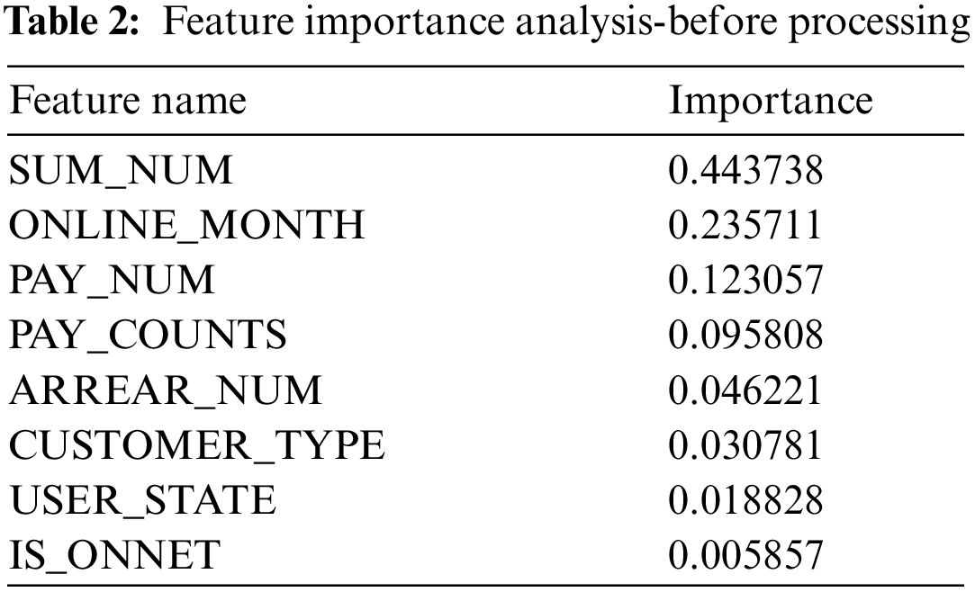
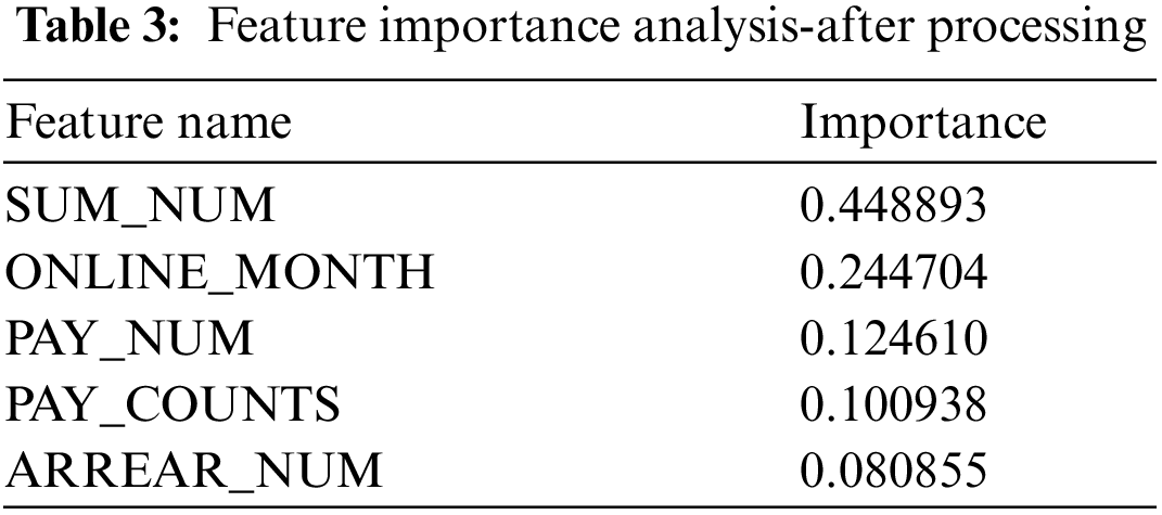
Use the Removing features with low variance method [14] to roughly filter the selected features, calculate the variance of each feature in the sample, and filter if it is lower than the set threshold. Pack the filtered features into a feature matrix and input the label together for model training, and calculate the weight coefficients of the trained data features. Based on this, the features are arranged in the order of weight coefficients from largest to smallest, and then the top features are selected. Taking the result of Decision Tree operation as an example, 8 features are input into the model training, and the feature importance ranking is shown in Tab. 2. Obviously, the weight coefficients of contract type, user status, and off-grid features are much lower than other features, indicating that these features do not have a great contribution and importance. On the contrary, they also caused an increase in the amount of data, which is not conducive to the training of the model. The feature importance results after removing the three features and then sending them to the model training are shown in Tab. 3. The remaining feature importance is not much different, and they all have a higher contribution to the model and are available for feature selection.

3.3 Model Training

This article will use Python language for model training. Taking account of the characteristics of the data set, classifier models such as Naive Bayes, Support Vector Machine, K-Nearest Neighbors, Decision Tree, Random Forest and XGBOOST model are selected. Use the corresponding modules in the Sklearn library for model training. The results of testing the model on the test set are shown in Tab. 4.

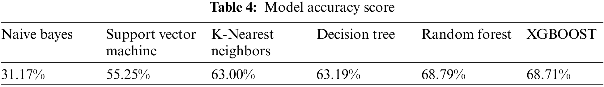
It can be seen that the Random Forest and XGBOOST models perform best, with an accuracy rate close to 70%. The worst effects are Naive Bayes and Support Vector Machine models, with an accuracy rate of less than 60%. Since the Random Forest and XGBOOST model are significantly better than other single models, and among the two models with good effects, Decision Tree and KNN, Decision Tree is more explanatory than KNN. This article chooses Decision Tree, Random Forest, and XGBOOST for optimization.

3.4 Model Optimization

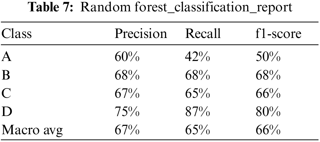
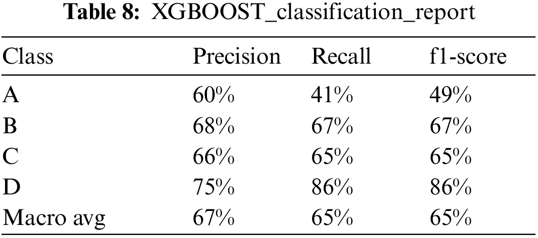
The training process of the machine learning model involves many hyper parameters. Choosing appropriate hyper parameters can improve the effect of the model. The optimization process of the model is the process of searching and selecting the optimal parameters. Train the model by setting the searched optimal parameters and test it on the test set. The results of the Decision Tree, Random Forest, and XGBOOST model are shown in Tabs. 5–8.

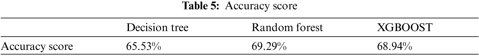
Comparing Tabs. 4 and 5, it can be seen that the effects of the three models have been improved through optimization. Among them, the most improved is the Decision Tree model, the prediction accuracy increased from 63.19% to 65.53%, an increase of 2.34%. Although the Random Forest and XGBOOST models are less improved than the Decision Tree model, they are still the best models. It can be seen that the integrated model has a better effect on credit rating.

4  Experimental Results

(1)   Accuracy

Run the model by setting the optimal parameters, and calculate the accuracy rates of Decision Tree, Random Forest, and XGBOOST on the test set to be 63.19%, 68.79%, and 68.71%, respectively.

(2)   Confusion matrix

The confusion matrices [15] of the test results of the Decision Tree, Random Forest, and XGBOOST model are shown in Figs. 3–5 respectively. The test data used by the three models is the same, with a total of about one million users, among which the numbers of A-level, B-level, C-level, and D-level users are 12875, 32337, 28216, and 30762, respectively. Because the number of the four levels is different, it is difficult to directly evaluate the confusion matrix simply by comparing it. Therefore, each element of the confusion matrix is divided by all the elements in the row to obtain the probability value, which is convenient for comparison and evaluation. By comparing the confusion matrix of the models, it can be found that the three models are able to distinguish D-level users (lower levels), but the effect of distinguishing A-level users (higher levels) is poor. It can be clearly seen from the figure that adjacent levels are more likely to be misjudged. This is because the information of users with similar credit levels is less different. Relatively speaking, for the A level, the Random Forest and XGBOOST are more accurate than the Decision Tree identification. For the B, C, D level, the Decision Tree recognition rate is not so different, but it is still not as effective as the other two models. In general, Random Forest and XGBOOST are effective in telecom rating problems.

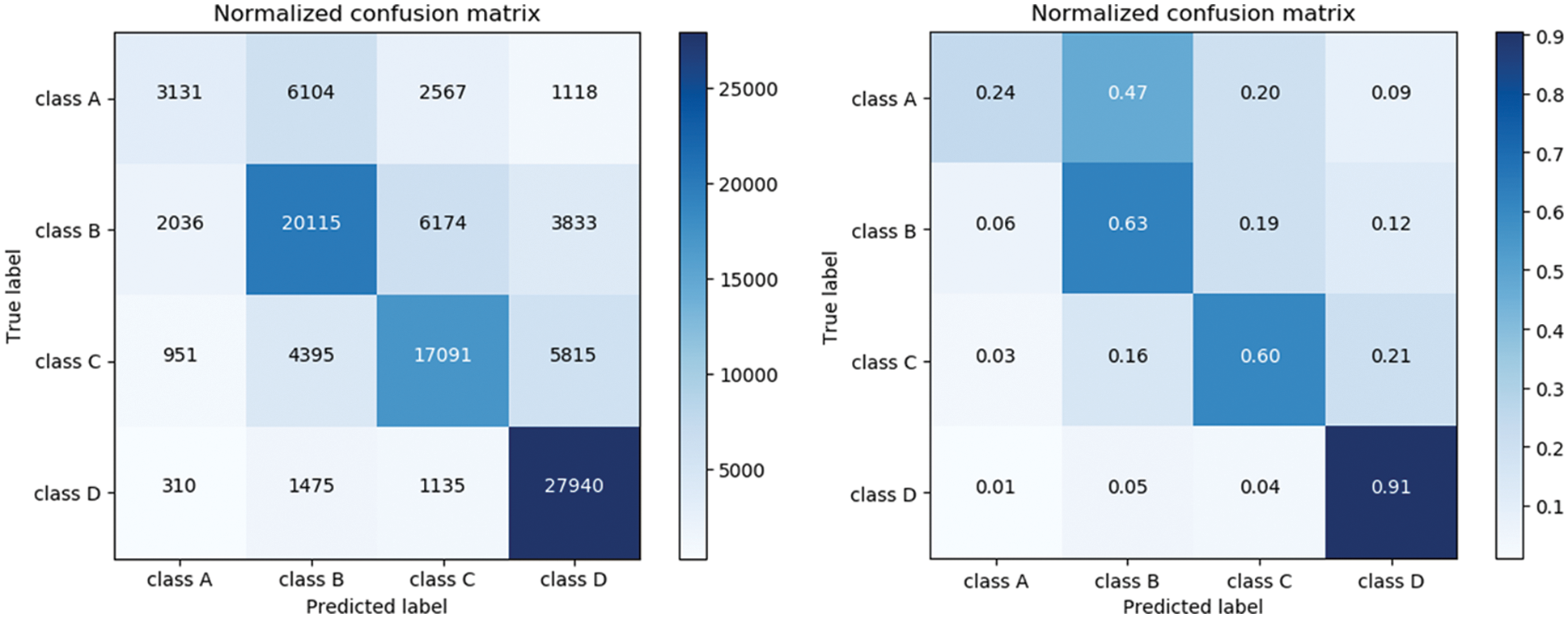
Figure 3: Decision tree_confusion matrix

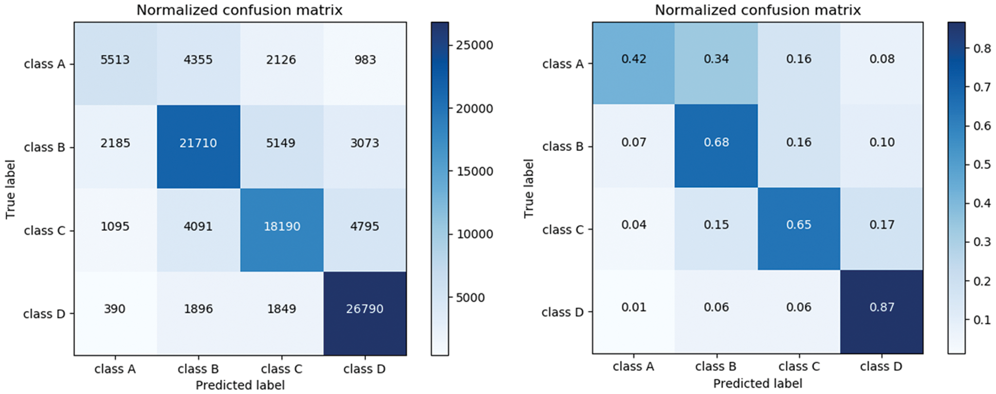
Figure 4: Random forest_confusion matrix

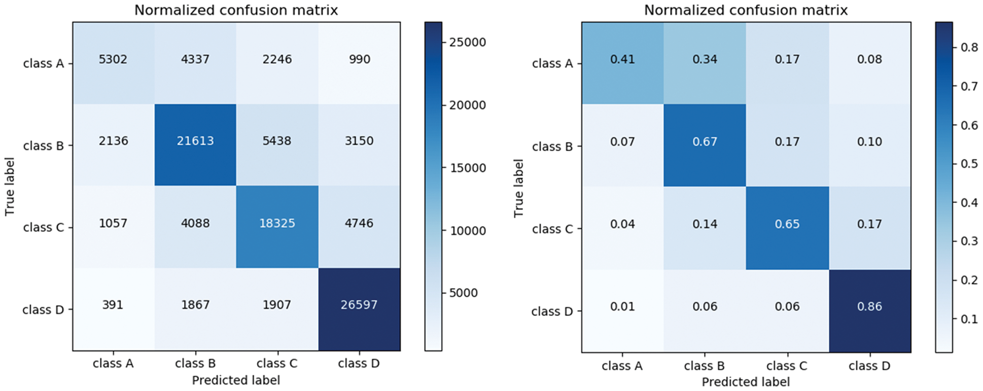
Figure 5: XGBOOST_confusion matrix

(3)   Recall, Precision, F1-score

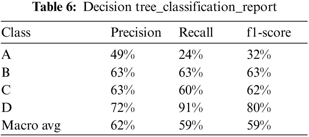
The following conclusions can be drawn from Tab. 6–8:

In terms of recall, precision, and f1-score [16], for the comparison of level test performance, the ranking of the three models is D level > B level ≈ C level > A level. For A, B, C, D grade and overall macro avg, Random Forest ≈ XGBOOST > Decision Tree. In other words, the three models can fully identify low-level users, and predict the low-level users correctly with a higher accuracy rate. Among them, the best model performance is Random Forest and XGBOOST.

In this paper, six basic classification model methods are tested successively, and the comparative experimental results show that random forest and XGBOOST achieve better classification effect of grade prediction. Therefore, an implementation scheme based on random forest, XGBOOST algorithm and model is proposed for telecom user rating.

5  Conclusion

This paper studies the machine learning algorithm used in telecom scenarios and proposes a method for predicting the credit rating of telecom users based on Random Forest and XGBOOST. Since the selected feature set changes with time, place, and social environment, the credit rating of telecom customers is a dynamic process. The model parameters should change with the time period and can be adjusted to ensure high prediction accuracy. Since the model itself is based on a time sliding window, it has a continuous learning process of historical and new data, can automatically learn and update parameters. In this paper, six classification models are established. Among them, the Decision Tree, Random Forest, and XGBOOST algorithm with better test results were selected for model optimization. Based on the optimization model, the test set is graded prediction, and the accuracy, confusion matrix, recall, precision, F-score and other indicators are calculated to obtain the Random Forest and the XGBOOST model has the best effect.

The experimental results show that the telecom user rating method based on Random Forest and XGBOOST can predict credit rating results with higher accuracy based on the given data, which can be used by operators to develop targeted marketing strategies. For example, the higher the credit rating, the higher the credit line, can reduce the problem of downtime due to not timely payment. Developing specific marketing strategies to retain customers who have low credit ratings and are extremely easy to leave the Internet will avoid huge losses caused by customer loss. Through the effective use of credit assessment, it can make up for the lack of personal credit investigation in other industries. Using accurate model identification can effectively replace manual evaluation and provide help for enterprise decision making. However, the accuracy of different levels of recognition varies greatly, and high-level users are poorly recognized. Models can be established for each level to improve the accuracy of each level, and finally model fusion is performed to obtain a level division result. This is a direction that can be considered for our future work.

Funding Statement: This work was supported by the National Natural Science Foundation of China (61871058).

Conflicts of Interest: The authors declare that they have no conflicts of interest to report regarding the present study.

This work is licensed under a Creative Commons Attribution 4.0 International License, which permits unrestricted use, distribution, and reproduction in any medium, provided the original work is properly cited.