Deep Learning: A Theoretical Framework with Applications in Cyberattack Detection

1  Introduction

Communication and control systems, including computers, sensor networks, and data centers, constitute the fundamental undergirding of modern society. The increasingly integrated global networks of sensors, actuators, computers, data centers, communication networks, software applications, and control systems, which are collectively labeled as information technology (IT) systems, handle the acquisition, production, storage, processing, and flow of sensitive and critical data related to personal, commercial, industrial, and government entities [1–3]. Among the myriad applications of IT systems are the control and monitoring of physical and industrial processes, including the electric power grid and virtually all other essential services. The industrial supervisory control and data acquisition (SCADA) systems govern the operation of public and industrial systems that directly affect people’s daily lives and the normal functioning of contemporary information-centric society [4]. The pervasive and growing interconnectivity of ubiquitous devices and systems, including sensors, data acquisition, storage, processing and communication modules, and actuators, amplify the complexity of IT systems [5–8]. Industrial control systems, including SCADA and other complex real-time sensing, communication, actuation, and control of web and application servers, databases, interfaces, switches, and routers, are distributed over wide geographic areas, and operate under incongruent standards, administrative regulations, and disparate jurisdictions [9].

The consistent availability, confidentiality, and integrity of the information that is generated, stored, accessed, processed, and transmitted through IT systems are fundamental and functional perquisites of modern society. As the world becomes increasingly interconnected and the industrial Internet of Things (IoT) proliferates globally, the production volume and flow speed of mission-critical data will accelerate. To deliver the expected value and services to their customers, clients, and constituents, commercial organizations, civil society, and governments will generate, store, access, transmit, update, and process vast quantities of data.

Bad actors, including criminal organizations and hostile governments, are constantly probing networks and exploiting the vulnerabilities of IT systems as a means to mount cyberattacks for financial gains, theft of intellectual property, espionage, and obtaining tactical and strategic advantages. Cyberattacks may involve theft, destruction, alteration, and encryption of data and processes, or disruption of normal services by unauthorized entities [10]. The increasing frequency, sophistication, and severity of cyberattacks demand the development of robust, agile, rapidly deployable, scalable, economical, low-power, and adaptive network intrusion detection systems.

A straightforward and effective cyber defense mechanism may involve arming the standard network packet capture and packet sniffer systems, which are routinely utilized for system administration and traffic analysis functions, with packet classifiers for the detection of malicious activity [11–13]. A binary packet classifier that is capable of real-time assignment of labels, namely benign (normal) or attack, to each packet constitutes an economical yet powerful first line of defense against various cyberattack modalities including DDoS and malware.

Packet classification is a standard process deployed on various network devices, including high-speed Internet routers and firewalls. Owing to the increasing diversity of network services, including data, voice, television, web hosting, live streaming, gaming, etc., packet classification to form proper packet flows, provide firewalls, and quality of service have become essential components of Internet routers. They are routinely used for packet filtering, traffic accounting, and other network services, including traffic shaping and service-aware routing, where packets are classified into differentiated traffic flows for providing application-specific quality of service [14,15]. The NN-based attack detector described in this paper is an additional packet classification layer that can be added to the existing routers’ packet classification algorithms. The fundamental difference between the NN classifier described in this paper and the rule-base packet classifiers in [14,15] is their underlying approach to making classification decisions. The rule-based classifiers rely mainly on the predefined procedures and instructions which are crafted by domain experts to make classification decisions. The NN classifiers, on the other hand, automatically discover the intricate patterns and hidden features of the data without explicit external guidelines provided by the user. The NN classifier described in this paper is capable of learning complex patterns and nonlinear relationships from data which makes it more effective and flexible. The proposed NN detector has low storage requirements and can be readily deployed in static random-access memory (SRAM), which provides the detector with flexibility and scalability.

2  Background

The development and implementation of cyberattack detection tools and mitigation strategies have been active areas of research for several decades [9,11] and [14–17]. Classical cybersecurity solutions include the utilization of access control methods such as identity and access management (IAM) tools; multifactor authentication techniques such as passwords, token-based authentication, and biometrics; data encryption; antimalware detection; endpoint protection; and firewalls [17–19].

Motivated by the biological brain’s remarkable ability to handle complex problems and information processing, researchers have dedicated several decades to developing artificial neural networks (ANNs) inspired by the structure and function of the brain [20–22]. Fundamentally, an NN is a massively parallel computational engine that is comprised of interconnected elementary analog processing nodes called neurons. The function of each node (neuron) is simply to compute the weighted sum of its various inputs and pass on the result through a non-linear activation function such as sigmoid [20–22]. The number of neural layers and nodes, the manner of interconnections among the nodes, and the weight coefficients assigned to the various connections in the network are the parameters that determine the network functionality. Although the initial inspirations responsible for the development of NN were primarily biological systems, they have proven their value for complex non-linear mapping as well as their practical applications to various problems in pattern recognition, signal processing, natural language processing, time-series prediction, and forecasting [19–23] and [24–26]. Because of their VLSI implementation, NN solutions are economical and can be deployed at scale [27]. Over the years, efficient learning algorithms have been devised to determine the NN weight coefficients [28].

In Section 3, the general framework of the feedforward multilayered perceptron is described. The computational complexity of the feedforward network is presented in Section 4. The process for computing the weights and biases of the feedforward multilayered network is explained in Section 5, where Sections 5.1 and 5.2 present, respectively, the input-output mapping function and the backpropagation algorithm. The training process used for the NN packet classifier is presented in Section 6. Section 7 describes the dataset used for training and testing the performance of the packet classifier. Test results are presented in Section 8. Conclusions and future research are presented in Section 9.

3  Feedforward Multilayered Perceptron Architecture

The binary classifier utilized here comprises a multi-layered perceptron (MLP), which is also called a feedforward neural network (FFNN), as shown in Fig. 1. In this section, we will briefly discuss the NN architecture and dynamics. The process of NN learning is achieved through gradient descent and backpropagation learning algorithms. The data processing progression from the network input to the output and the learning algorithm are succinctly reviewed in Section 4. The derivations and detailed formulations of the backpropagation algorithm are given in Section 5.

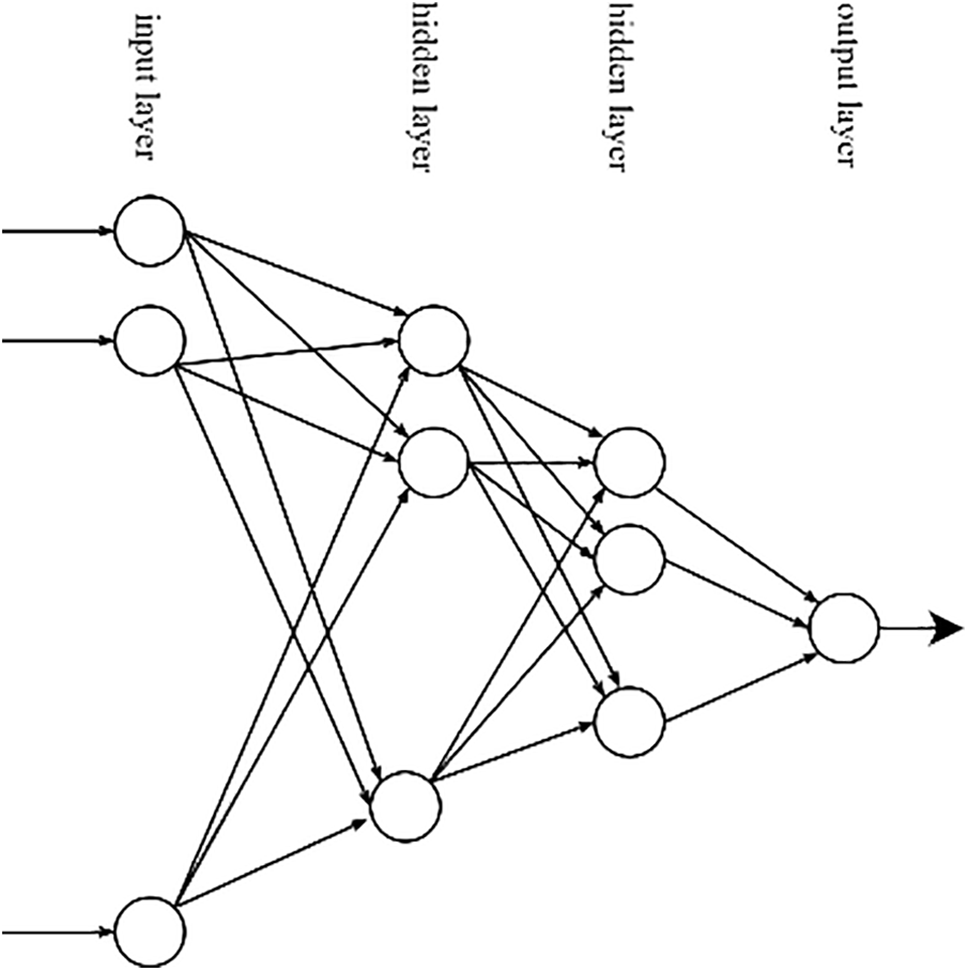
Figure 1: Fully connected feedforward neural network

A typical FFNN is comprised of an input layer, an output layer, and one or more hidden layers. The input and output layers are the visible layers of the network, and all the other layers are called hidden layers. The reason for employing the term “hidden” for the layers sandwiched between the input and the output layers is that in an NN classifier, during the training phase, for each training vector at the input, the desired responses of the output layer neurons are known, whereas the desired outputs of the neurons in the hidden layers are not known a priori. Each layer is comprised of several neurons, which are also called nodes. In a fully connected network, each of the nodes (neurons) in a typical layer is connected to all the nodes in the next layer.

The data processing steps progress from the input layer on the left to the output layer on the right, as shown in Fig. 1. The number of nodes in the input layer is dictated by the dimensionality of the input feature vectors, which the network is designed to process. The number of nodes in the output layer is determined by the functionality of the network. For example, a network that is intended for binary classification of input data has only one node at the output layer. Likewise, the number of nodes in the output layer of a NN classifier with K distinct classes is K. The number of hidden layers in the NN and the number of nodes in each of the hidden layers are application-dependent and are determined by standard optimization techniques or trial and error.

Fig. 1 shows an FFNN, where the nodes in the left column and the rightmost node comprise the visible layers of the network and denote, respectively, the input layer and the output layer. All the other layers between the input layer and the output layer are hidden layers. Two operations are performed at each node: (i) the weighted sum of the outputs of all the nodes in the preceding layer is computed at the node input and a bias is added to form the input signal; (ii) the node applies a nonlinear activation function to the signal at its input to generate the output signal.

4  Computational Complexity of the Feedforward Neural Network

In a fully connected FFNN, the input of a typical node is the weighted sum of the outputs of all the nodes in the preceding layer added to the bias factor of the node under consideration. The activation (output) of the neuron is expressed by Eq. (1).

yi(k)=f[(∑j=1Nk−1wij(k)yj(k−1))+bi(k)];1≤k≤K,1≤i≤Nk.(1)

where k, i denote, respectively, the layer-index and the index of the neuron within the layer; yi(k) denotes the output (activation) of the ith neuron of the kth layer; wij(k) denotes the weight factor associated with the connection between the jth neuron of the (k – 1)th layer and the ith neuron of the kth layer; bi(k) denotes the bias factor or threshold associated with the ith neuron of the kth layer; Nk−1 denotes the number of nodes in the (k – 1)th layer; K denotes the total number of layers; Nk denotes the number of nodes in the kth layer; and f represents the non-linear neural activation function.

The input layer is considered the zeroth layer, and the outputs of the input layer nodes (neurons) are the same as the corresponding components of the input feature vector, which is to be processed by the network. The nodes of the input layer, the 0th-layer, simply pass on the signals applied at their inputs to their respective outputs yi(0)=xi. The neural activation function f can be any non-linear function. Examples of activation functions are defined below in Eqs. (2a)–(2f) and are plotted in Fig. 2.

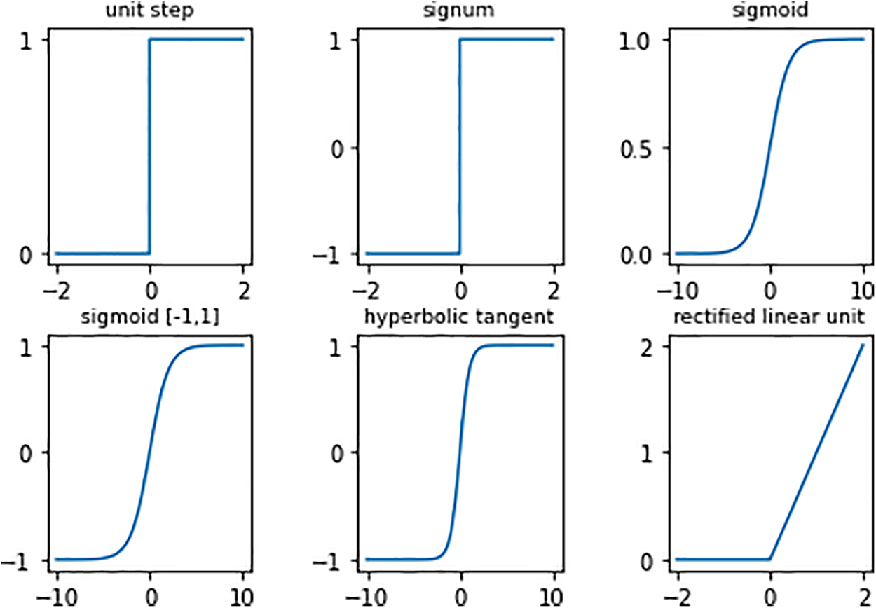
Figure 2: Typical non-linear activation functions

unit step function:f(x)={1;x≥00;x<0.(2a)

signum function:f(x)={1;x≥0−1;x<0.(2b)

sigmoid function:f(x)=11+e−x.(2c)

modified sigmoid function [−1,1]:f(x)=1−e−x1+e−x.(2d)

hyperbolic tangent function:f(x)=e2x−1e2x+1.(2e)

rectified linear unit function ReLU:f(x)={x;x≥00;x<0.(2f)

Fig. 3 shows a typical node in a typical layer, namely the ith node in the kth layer of the network and its connections to the nodes in the preceding layer, including the weights and the bias factor. The activation (output) of the node is expressed by Eq. (1) above. The meaning of the symbols in Fig. 3 is explained right after Eq. (1). The matrix expression of Eq. (3) provides the relationship between the outputs of all the Nk nodes in the kth layer of the network and the outputs of the Nk−1 nodes of the (k – 1)th layer.

Figure 3: The input of the ith neuron in the kth layer of the feedforward network

In Eq. (3a) the superscript k refers to the layer-index in the network; f represents the neural activation function; Y(k) is a column vector with length of (Nk+1) containing the outputs of all the nodes in the kth layer prepended with one; Y(k−1) is a column vector with length of (Nk−1+1) containing the outputs of all the nodes in the (k – 1)th layer prepended with one; and W(k) is a matrix with dimensions Nk×(Nk−1+1) containing all the weight coefficients and bias factors associated with the connections to the inputs of the nodes in the kth layer of the network.

Y(k)=f(W(k)Y(k−1)).(3a)

Y(k)=[1y1(k)...yNk(k)], Y(k−1)=[1y1(k−1)...yNk−1(k−1)].(3b)

W(k)=[b1(k)w1,1(k)w1,2(k)…w1,Nk−1(k)⋮bNk(k)wNk,1(k)wNk,2(k)…wNk,Nk−1(k)].(3c)

In Eq. (3a), the activation function f is vectorized so that it operates on each component of its argument, which is a column vector. As seen from Eqs. (3a)–(3c), the NN processes the incoming data applied to the network input, which is also denoted as the zeroth layer, by a sequence of matrix multiplications followed by the nonlinear neural activation operations. Specifically, the input data represented as a column vector is multiplied with W(1), which denotes the weight-bias matrix of the first hidden layer, and the result of the matrix multiplication is subsequently operated upon by the activation function f. The result of this operation is then multiplied with W(2) and subsequently operated upon by f, and so on, until the last layer is reached, and the NN output is computed.

It is seen from above that the number of matrix multiplications required to compute the network response to the input data is equal to (K + 1), where K represents the number of hidden layers. The number of algebraic operations and the computation of the neural activation functions required for the processing of a typical feature vector applied to the input of the NN are given below:

Pmults.,adds.=N1(D+1)+∑k=1KNk+1(Nk+1).(4a)

Pf=∑k=1K+1Nk.(4b)

where Pmults.,adds., Pf denote, respectively, the number of decimal additions-multiplications, and the number of activation function evaluations. The number of features (components) of the input vector is denoted as D; the number of hidden layers comprising the neural network is K; Nk denotes the number of nodes in the kth layer of the network; and the subscript K+1 denotes the output layer.

5  Multilayered Feedforward Neural Network Training

This section provides a detailed block diagram representation of the fully connected, multilayered FFNN. The complete mathematical formulations of the forward pass for modeling the network operations on the input data are given. The derivations of mathematical formulas used in the backpropagation operation are also given. Formulas for the computation of the loss (cost) function and its relationship to the network weights and biases are derived. The relationship between errors at the outputs of the neurons in consecutive layers of the network is formulated. The detailed exposition of the backpropagation algorithm, which is used for training the NN is discussed. The nomenclature employed in this section uses explicit symbols for the weights and biases, which are different from the notations in Section 3.

5.1 Forward Pass Operation of the Multilayered Perceptron

The block diagram representation of the FFNN is shown in Fig. 4, where the network consists of the input layer, the output layer, and l hidden layers. In a typical NN, the number of hidden layers is equal to or greater than one. The hidden layers are designated by their indices, one through l, where indices one and l denote, respectively, the first and the last hidden layers. The input layer is also called the zeroth layer, and the output layer is the (l + 1)th layer.

Figure 4: Block diagram representation of the multilayered feedforward neural network

Each of the hidden layers and the output layer, namely layers one through (l + 1), consist of a set of neurons, which are also called nodes, where rk denotes the number of neurons (nodes) in the kth layer, including the hidden layers 1≤k≤l, and the output layer k=l+1. The input layer has r0 nodes, the outputs of which are the components of the feature vector representing the input data applied to the NN. Each layer is fully connected to the layer that immediately follows it. This means all the neurons (nodes) of the input layer as well as all the nodes of each hidden layer are connected to every neuron in the next layer. There are no connections between the neurons of the same layer. The neural connections are unidirectional, and signals propagate from neurons of each layer to the neurons of the next layer from left to right. In Fig. 4, column vectors are represented by underlined bold lowercase letters, matrices are represented by bold block letters, and the meaning of each symbol is explained in the following paragraphs.

The input and output of the kth hidden layer, 1≤k≤l, are column vectors of length rk, which are, respectively, designated as a→(k),o→(k) in the following analysis, and are denoted in Fig. 4 as a_(k), o_(k). Each element of the output vector at the kth hidden layer is obtained from the corresponding element of the hidden layer’s input vector operated upon by the neural activation function. The input layer of the block diagram of Fig. 4 at the upper-left, which is also called the zeroth layer, simply passes the vector applied to the input of the NN to the output of the zeroth layer. In all the other layers, however, two operations are performed. In each layer, the inputs of the neurons are computed as the weighted sum of the outputs of all the neurons in the preceding layer plus the bias vector. The output of each neuron is then computed by applying a nonlinear activation function, such as sigmoid or ReLU, to the input of the neuron.

a→(k)=[a1(k),a2(k),…,ark(k)]T,o→(k)=[o1(k),o2(k),…,ork(k)]T.(5a)

o→(k)=σ(a→(k)),oi(k)=σ(ai(k)),1≤i≤rk.(5b)

where a→(k), o→(k) denote, respectively, the input and output vectors at the kth layer in Fig. 4, the superscript T denotes matrix transpose, the subscripts refer to vector components, and σ denotes the neural activation function, for example, the sigmoid function of Eq. (2c). In the block diagram of Fig. 4, a line connecting a pair of consecutive layers, for example, the (k−1)th and kth layers, comprises rk×rk−1 weighted connections, which is represented by the weight matrix W(k). Where, rk−1, rk denote the number of neurons in two consecutive layers. The input vector of the kth layer is obtained from the output vector of the (k−1)th layer by Eq. (6) below:

a→(k)=W(k)o→(k−1)+b→(k);1≤k≤l+1.(6a)

o→(k−1)=[o1(k−1),o2(k−1),…,ork−1(k−1)]T;1≤k≤l+1.(6b)

W(k)=[w1,1(k)w1,2(k)…w1,rk−1(k)w2,1(k)w2,2(k)…w2,rk−1(k)⋮wrk,1(k)wrk,2(k)…wrk,rk−1(k)],b→(k)=[b1(k),b2(k),…,brk(k)]T.(6c)

where l is the number of hidden layers. In Eq. (6a), the terms on the right hand side, W(k), o→(k−1), b→(k), are matrices with dimension of, respectively, (rk×rk−1), (rk−1×1), (rk×1), and the term on the left hand side is a column matrix with (rk×1) dimensions, whose components are expressed below:

ai(k)=bi(k)+∑j=1rk−1wij(k)oj(k−1);1≤i≤rk.(7)

where ai(k) denotes the ith element of the input vector to the kth layer of the network; oj(k−1) is the jth element of the vector at the output of the (k – 1)th network layer; wij(k) denotes the value of the ith row and jth column of the weight matrix W(k); bi(k) is the ith element of the bias matrix b→(k); and rk−1, rk denote the number of neurons in the (k – 1)th and kth network layers. Here, the weight and the bias matrices are associated with the connections between the (k – 1)th and kth layers of the block diagram of Fig. 4. It is also noted that ai(k), oj(k−1) are, respectively, the signal at the input of the ith neuron of the kth layer, and the signal at the output of the jth neuron of the (k – 1)th layer. It is further noted that wij(k) is the weight factor associated with the connection from the jth neuron of the (k – 1)th layer to the ith neuron of the kth layer, and bi(k) is the bias factor of the ith neuron of the kth layer.

To compute the response of the neural network to an input vector, we start at the input layer, and analyze the cascade effect of consecutive layers of the network on the input vector. The input layer (zeroth layer) passes through the applied vector to the output of the zeroth layer without doing anything to it. In the block diagram of Fig. 4, the output of the input layer, which is also called the zeroth layer, is set equal to the vector applied to the input of the neural network.

o→(0)=x→.(8)

where x→,o→(0) denote, respectively, the vector applied to the network and the output of the zeroth layer. The output of the zeroth layer (input layer) together with the weight and bias matrices of the first hidden layer are used to compute the input matrix of the 1st hidden layer. The output matrix of the 1st hidden layer is then computed from its input. The operations for computing the input and output matrices associated with the 1st hidden layer are given in Eqs. (9a), (9b).

a→(1)=W(1)o→(0)+b→(1)=W(1)x→+b→(1).(9a)

o→(1)=σ(a→(1))=σ(W(1)x→+b→(1)).(9b)

a→(2)=W(2)o→(1)+b→(2)=W(2)(σ(W(1)x→+b→(1)))+b→(2).(10a)

o→(2)=σ(a→(2))=σ(W(2)(σ(W(1)x→+b→(1)))+b→(2)).(10b)

Using the output of the 2nd hidden layer, the input of the 3rd hidden layer and subsequently its output are computed as shown in Eqs. (11a), (11b).

a→(3)=W(3)o→(2)+b→(3)=W(3)(σ(W(2)(σ(W(1)x→+b→(1)))+b→(2)))+b→(3).(11a)

o→(3)=σ(a→(3))=σ(W(3)(σ(W(2)(σ(W(1)x→+b→(1)))+b→(2)))+b→(3)).(11b)

Continuing the iterative process of using the output of a layer to compute the input of the next layer and subsequently the layer output, one arrives at the expression for the output of (l + 1)th layer which represents the response of the NN to the input x→ as shown in Eqs. (12a), (12b).

o→(l+1)=σ(W(l+1)σ(W(l)σ(W(l−1)σ(…σ(W(1)x→+b→(1))+b→(2))…+b→(l−1))+b→(l))+b→(l+1)).(12a)

y→^=o→(l+1).(12b)

where y→^ represents the response of the NN of Fig. 4 to the input x→. The matrices W(k), b→(k) denote the weight and bias matrices associated with the kth layer of the network, where 1≤k≤l+1, and l is the number of hidden layers which is equal to or greater than one. In the expression of Eq. (12a), the neural activation function σ is assumed to be the same across all the layers, which does not need to be the case. The activation function of each layer can be any one of the nonlinear functions given in Eqs. (2a)–(2f). In the experiments of Sections 6–8, the activation functions utilized across all the hidden layers are the ReLU function of Eq. (2f), and the activation function of the output layer is the sigmoid function of Eq. (2c).

Eq. (12a), which transforms the input vector x→ to the output vector o→(l+1), is a composition function, transforming the r0 dimensional vectors at the input to the corresponding rl+1 dimensional vectors at the output of the network. The linear operations W(k)o(k−1)+b→(k) are affine transformations, which map hyperplanes with rk−1 dimensions in one space to hyperplanes with rk dimensions in another space. If the nonlinear activation function is chosen to be ReLU, σ(W(k)o(k−1)+b→(k)) represents folding of the hyperplane in the second space, where each hyperplane has a single fold. Therefore, each layer of the network transforms the input of the layer through affine transformation and folding. The overall effect of the multilayered perceptron is creating continuous piecewise linear functions. The transformation is represented by folded hyperplanes. The number of folds in each hyperplane is equal to the sum of binomial factors ∑q=0r0(l+1q), where l+1 is the number of layers and r0 is input dimensionality.

The number of layers and the number of neurons in each of the layers of the network, which constitute the architecture of the multilayered FFNN, as well as the neural activation functions are design parameters which are application dependent. For example, in a NN designed for a classification application the number of neurons of the input layer equals the dimensionality of the feature vector representation of the input data to be classified. The number of neurons of the output layer is determined by the number of classes. For instance, a binary classifier has only one neuron at the output layer. The number of hidden layers and the number of neurons in each hidden layer are set heuristically by the designer. The values of the weights and biases are computed by applying the multilayered feedforward perceptron learning algorithm which involves a training set comprised of a set of input feature vectors and the associated known classes.

5.2 Multilayered Perceptron Learning Algorithm

The training process of the neural network classifier involves the computation of the weight and bias matrices using a given training set. The training set is comprised of a finite set of training vectors and their corresponding classes. The number of nodes at the input layer r0 in Fig. 4 is equal to the dimensionality of the training vector, and the number of nodes at the output layer rl+1 is dependent on the number of classes of the classification problem for which the network is designed. For example, consider a specific training vector x→ that belongs to class j(1≤j≤rl+1) and is applied to the network input at the 0th layer (input layer). Because it belongs to class j, the output of the jth neuron at the output layer must be one, and the outputs of all the other neurons in that layer must be zero. This desired output, which is also called the target, represents the ground-truth, and is different from the actual output computed by the NN. The actual output of the network is computed by applying the feedforward process of Eqs. (12a), (12b) to the input vector. The difference between the target output and the computed (actual) output, which is called the error at the output layer, is subsequently used to update the weights and biases of the network using the gradient descent and backpropagation algorithms, which are detailed below.

The stochastic gradient descent (SGD) process involves applying one trainer at a time to the neural network and updating the network weights and biases accordingly. The trainers are applied one at a time, and the output is computed; the computed output is compared to the target output or ground-truth as specified by the training set; the difference between the computed output (actual output in response to the input) and the target output is used to update the weights and biases. This process is repeated for each trainer in the training set. The execution of the training process for all the vectors in the training set is called one training epoch. The training process is repeated for a user-prescribed number of training epochs, until all the trainers are classified correctly or until the relative changes in the weights and biases fall below the user-prescribed thresholds. The error, which is also called the loss or cost function, associated with one trainer is given by Eq. (13).

E=O→(l+1)−y→.(13)

where O→(l+1) is the actual response of the NN in Fig. 4 to the trainer feature vector x→ applied at the input of the network, and y→ is the target output (ground-truth). The pair of vectors x→, and y→ comprise one training instant. The components of the response vector O→(l+1) in the loss function expression of Eq. (13) are given below:

oi(l+1)=σ(ai(l+1));ai(l+1)=bi(l+1)+∑j=1rlwij(l+1)oj(l).(14)

where ai(l+1), oi(l+1) denote, respectively, the input and the output of the ith neuron of the (l+1)th layer; σ is the neural activation function; bi(l+1), wij(l+1) denote, respectively, the bias of the ith neuron of the (l+1)th layer and the weight coefficient associated with the connection from the jth neuron of the lth layer to the ith neuron of the (l+1)th layer; oj(l) is the output of the jth neuron of the lth layer; and rl is the number of nodes in the lth layer. It is noted that the (l+1)th layer is the output layer.

From Eq. (13), it is seen that the loss (cost) is affected by the difference between the actual responses of the output layer neurons (oi(l+1);1≤i≤rl+1) and the target (desired) responses at the output layer neuron (yi;1≤i≤rl+1), which are known a priori for each of the training vectors x→ applied to the input of the network. The training process of the neural network involves the adjustment or updating of the weights and biases of the neural network in Fig. 4, namely, wij(k), bi(k), 1≤k≤l+1, 1≤i≤rk+1, 1≤j≤rk, to minimize the cost function of Eq. (13). It is noted that the weights and biases affect the cost function (loss function) through affecting oi(l+1) and they have no effect on yi.

The minimization of the cost function is achieved through the gradient descent process. The formulation of the gradient of the cost function involves derivation of the partial derivatives of the responses of the output-layer neurons oi(l+1) with respect to the network’s weights and biases. The expressions for the partial derivatives of the cost function with respect to the output layer weights and biases are obtained by applying chain rule as shown below:

∂E∂wij(l+1)=∂E∂oi(l+1)∂oi(l+1)∂ai(l+1)∂ai(l+1)∂wij(l+1),∂E∂bi(l+1)=∂E∂oi(l+1)∂oi(l+1)∂ai(l+1)∂ai(l+1)∂bi(l+1).(15)

The partial derivatives on the right-hand sides of the expressions of Eq. (15) are given by Eqs. (16a)–(16c).

∂E∂oi(l+1)=oi(l+1)−yi.(16a)

∂oi(l+1)∂ai(l+1)=σ(ai(l+1))(1−σ(ai(l+1)))=oi(l+1)(1−oi(l+1)).(16b)

∂ai(l+1)∂wij(l+1)=oj(l),∂ai(l+1)∂bi(l+1)=1.(16c)

The neural activation function is assumed to be the sigmoid of Eq. (2c), and its derivative is given in Eq. (17).

σ(x)=11+e−x,dσ(x)dx=σ(x)(1−σ(x)).(17)

Substituting from Eq. (16) into Eq. (15) and using Eq. (17), one arrives at the expressions for the partial derivatives of the cost function with respect to the weights and biases of the output layer as shown in Eqs. (18a), (18b).

∂E∂wij(l+1)=(oi(l+1)−yi)oi(l+1)(1−oi(l+1))oj(l).(18a)

∂E∂bi(l+1)=(oi(l+1)−yi)oi(l+1)(1−oi(l+1)).(18b)

δi(l+1)=oi(l+1)(1−oi(l+1))(oi(l+1)−yi).(19a)

∂E∂wij(l+1)=δi(l+1)oj(l).(19b)

∂E∂bi(l+1)=δi(l+1).(19c)

Using gradient descent, the procedures for updating the weights and biases of the output layer are expressed by Eqs. (20a), (20b).

wij(l+1)←wij(l+1)−γδi(l+1)oj(l).(20a)

bi(l+1)←bi(l+1)−γδi(l+1).(20b)

where the parameter γ is a user-prescribed small number, i.e., γ=0.1, called the learning rate. Eqs. (20a), (20b) provide a procedure for updating the output layer weights and biases after computing the response vector y→^=o→(l+1) of the network to the training input x→.

The derivations of the expressions of Eqs. (20a), (20b) for updating of the weights and biases of the output layer are straightforward, because the error terms at the outputs of the neurons of the output layer are known. As seen in Eq. (19a), δi(l+1) can be computed directly, because yi, which denotes the desired (target) output of the ith neuron in the output layer, is known from the training set. This, however, is not the case for the hidden layers. The desired outputs of the neurons in the hidden layers are not known directly, which is the reason they are called hidden layers.

The error terms at the outputs of the neurons of the hidden layers are not directly known, because unlike the output layer, for which the target values of the outputs of the neurons are known a priori, the target values of the outputs of the neurons of the hidden layers are not known. To determine the partial derivatives of the cost function with respect to the weights and biases of the hidden layers, one must first determine the errors at the outputs of the neurons of the hidden layers. This is where the concept of back propagation originates. Knowing the errors at the outputs of the neurons of the output layer, the errors are propagated backward to compute the errors at the outputs of the neurons of the hidden layers, one layer at a time.

The backpropagation process is illustrated by formulating the partial derivative of the cost function of Eq. (13) with respect to a typical weight factor of the lth layer, namely wjp(l). As seen in Fig. 5, wjp(l) denotes the weight coefficient associated with the connection between pth neuron of the (l-1)th layer and the jth neuron of the lth layer. It is noted that wjp(l), although affecting only one neuron in the lth layer, namely the jth neuron, it affects all the neurons in the output layer. This is because the jth node of the lth layer is connected to all the nodes of the output layer. Applying chain rule, the partial derivative of the coast function with respect to wjp(l) is obtained as below:

∂E∂wjp(l)=∑i=1rl+1∂E∂oi(l+1)∂oi(l+1)∂ai(l+1)∂ai(l+1)∂oj(l)∂oj(l)∂aj(l)∂aj(l)∂wjp(l).(21a)

∂E∂oi(l+1)=oi(l+1)−yi.(21b)

∂oi(l+1)∂ai(l+1)=oi(l+1)(1−oi(l+1)).(21c)

∂ai(l+1)∂oj(l)=wij(l+1).(21d)

∂oj(l)∂aj(l)=oj(l)(1−oj(l)).(21e)

∂aj(l)wjp(l)=op(l−1).(21f)

Figure 5: Illustration of backpropagation

Substituting Eqs. (21b)–(21f) in Eq. (21a) and rearranging terms one obtains the following:

∂E∂wjp(l)=oj(l)(1−oj(l))op(l−1)∑i=1rl+1[oi(l+1)(1−oi(l+1))(oi(l+1)−yi)]wij(l+1).(22)

Substituting from Eq. (19a) in Eq. (22), and rearranging terms leads to the following:

∂E∂wjp(l)=[oj(l)(1−oj(l))∑i=1rl+1wij(l+1)δi(l+1)]op(l−1).(23)

The bracketed term in Eq. (23) is called the error at the output of the jth neuron of the lth layer, as given below:

δj(l)=oj(l)(1−oj(l))∑i=1rl+1wij(l+1)δi(l+1).(24)

Eq. (24) shows how the error at the output of any layer can be obtained in terms of the error at the output of the next layer. This equation describes the backpropagation process, where the known error at the output of the network is propagated backward, one layer at a time, to obtain the error at the outputs of all the other layers including the hidden layers and the input layer. After computing all the δj(k) terms for a typical layer, the ∂E∂wjp(k−1) terms at preceding layer are computed, and this process starts at the output layer and proceeds all the way to input layer, one layer at a time. Following the computation of all the partial derivatives (gradients) the change values for all the weights and biases are recorded as expressed by Eqs. (25a)–(25c).

δj(k)=oj(k)(1−oj(k))∑i=1rk+1wij(k+1)δi(k+1); 1≤k≤l, 1≤j≤rk.(25a)

wij(k)←wij(k)−γδi(k)oj(k−1).(25b)

bi(k)←bi(k)−γδi(k).(25c)

6  Training the Neural Network

The values of the NN weights and biases are initially set randomly using a random number generator and a probability distribution function such as a normal distribution with zero mean and unit standard deviation. The training set is utilized to compute the NN weights and biases through the process of training the network, as described below.

For an NN classifier, the training set comprises a finite set of tuples, where each tuple consists of a feature vector and the corresponding class label comprising one training object. For example, the training set of a binary classifier comprises a set of feature vectors and the respective class labels, where each label can be either zero or one. The training vectors are applied to the NN classifier, one trainer at a time. The computed class label, which is the actual NN response to the feature vector representation of the training object, is compared to the true class label of the trainer. The true class label of the input feature vector, which is also called the ground truth, is the desired or target response.

According to the terminology in Section 5.2, the feature vector representation of the training object is denoted as x→, which is applied to the NN input. The computed response (actual response) of the NN to the training object is denoted as o→(l+1). The desired (target) response is the true class label of the training object and is denoted as y→. The pair of vectors comprising the feature vector of the training object and the respective class (x→, y→) comprise one training instant. For a binary classifier, the output layer of the NN has only one neuron, and the computed response is a scaler. The desired (target) response or ground truth is a binary number, zero or one, which is the true class label of x→.

The process of updating the weights and biases of a typical binary classifier proceeds as follows. The training object feature vector x→ is applied to the NN, and the scalar response of the network o(l + 1) is computed. The computed (actual) response o(l + 1) of the network and the true class label of x→, which is the binary number y are compared. Eqs. (19a), (20a), (20b) are used to update the weights and biases associated with the last layer, which is the (l + 1)th layer of the NN. The error term at the output of the (l + 1)th layer, δ(l+1) which is computed in accordance with Eq. (19a) is backpropagated, one layer at a time, to compute the error vectors δ→(k) at the output of every other layer using Eq. (25a). Eqs. (25b), (25c) are subsequently used to update the weights and biases at every layer. The procedure of computing the error vector at the output of the kth layer, namely, δ→(k) and updating of the weights and biases of that layer W→(k),b→(k) is done one layer at a time, starting from the output layer, and proceeding to the left. The weight and bias updating procedure outlined above is repeated for every training object in the training set. Each time, one trainer is applied to the NN, the weights and biases are updated, and the trainer is set aside. Then the next trainer is applied, the NN weights and biases are updated, and so on, until all the trainers have been utilized and the trainer set is empty. This constitutes one training epoch. The procedure is repeated for a user-prescribed number of training epochs, for example one hundred. At the end of each epoch, the order of trainers in the training set is shuffled randomly. The method of training described above is called stochastic gradient descent, and is the method used to obtain the experimental results reported in Section 7.

There are several other alternative training methods. In batch training, all the training elements are applied to the classifier, one trainer at a time as is done in stochastic gradient descent. After applying each trainer to the network, the actual network response to the trainer input is computed and is compared to the true class of the object as was done before. The backpropagation algorithm is used to compute and record the prescribed changes for all the weights and biases of the network without making any updates to the values of the weights and biases. After applying the entire training set to the NN and recording the prescribed changes of the weights and biases for each input, the change records across all trainers are combined and the weights and biases are updated at once at the end of the epoch. This process is repeated for a prescribed number of epochs.

The minibatch training method contains elements from both the stochastic training and the batch training. Here, multiple subsets of the training set each comprising a small number of trainers, for example one hundred trainers, are chosen randomly. Each randomly chosen subset is called a minibatch. Each of the randomly chosen minibatches are used to train the NN using the batch training method described above. There are several alternative ways to do minibatch training. In minibatch training without replacement, after a minibatch is utilized to train the NN, the trainers in the minibatch are removed from the training set, and the next minibatch is chosen from the remaining training set. In minibatch training with replacement, after a minibatch is utilized to train the NN, the trainers in the minibatch are put back into the training set, the set is reshuffled and the next minibatch is chosen and the training process continues.

7  Dataset

The multilayered feedforward neural network described in Section 4 is utilized as a classifier for cybersecurity applications. The NN is designed as a binary classifier to label the network traffic packets as either normal or an attack. The binary classifier is trained and tested using the KDD99 dataset, which has been widely utilized in cybersecurity studies. The KDD dataset is comprised of packet header data for 805,051 packets and is divided into two subsets, namely the training set and the test set. The training set comprises 494,022 packets, including 97,278 normal packets and 396,744 attack packets. The test set comprises 311,029 packets, including 60,593 normal packets and 250,436 attack packets. The attack packets in the training and test sets include four attack types: denial of service (DoS), probe attack, remote to local attack (R2L), and user to root attack (U2R). Each of the header packets in the training and test sets has forty-two attributes, including the packet label. Thirty-eight of the attributes are numerical, and three are categorical. In the work reported here, all the packets associated with the two main subsets of the KDD99 dataset, namely the training set and the test set, were combined into one dataset. The three non-numerical features of each packet header were dropped, leaving a dataset with 805,051 packets, where each packet has thirty-eight features and one binary label of normal or attack. The data set was then partitioned into two separate sets in accordance with the packets’ binary labels. The normal packets were all grouped together into the normal set, which contains 157,871 packets. Likewise, the attack packets were grouped together into the attack set, which contains 647,180 packets.

In the experiments reported in Section 8, the input applied to the classifier is a typical network traffic packet header. Each input is represented by its feature vector, which has thirty-eight dimensions. Each input can have one of two possible class labels, namely normal or attack. Therefore, the NN binary classifier has thirty-eight nodes in the input layer and one node in the output layer. The number of hidden layers and the number of nodes in each hidden layer are design parameters, that are determined through experimentation by trial and error heuristically. The training and test sets that are used to train the binary classifier and evaluate its performance were chosen from the normal and attack sets described in the previous paragraph.

8  Test Results

The packet classifier used in the experiments of this section is a multilayered feedforward neural network comprising an input layer with thirty-eight nodes, an output layer with one node, and l hidden layers. The hidden layers are numbered from one through l, and the number of nodes in each hidden layer is denoted as rk, where 1≤k≤l denotes the index of the hidden layer as shown in the block diagram of Fig. 4.

The NN training process involves a training set comprising normal and attack packets, which are randomly chosen from the normal and attack sets described in Section 7. In all of the experiments presented here, the number of normal and attack packets in the training set of each experiment are equal. Following the training process, the NN is tested by evaluating its performance using a test set. The test set also comprises normal and attack packets, which are randomly selected from the normal and attack sets of Section 7, after the removal of the training packets from each set. In all the experiments presented here, the number of normal and attack packets in the test set of each experiment are equal. Each of the packets of the test set is applied to the trained classifier, and the classifier computes the class label for each test packet. The computed class of each test packet is compared to the respective true class. If the true class of the input packet (ground truth) is attack and the computed class is also attack, this is called true-positive (TP). If the true class of the input packet is attack but the computed class is normal, this is called false-negative (FN). If the true class of the input packet is normal and the computed class is also normal, this is called true-negative (TN). If the true class of the input packet is normal but the computed class is attack, this is called false-positive (FP). These definitions are further illustrated by Eqs. (26a), (26b) and Table 1.

TP+FN=total number of attack packets in the test set(26a)

TN+FP=total number of normal packets in the test set(26b)

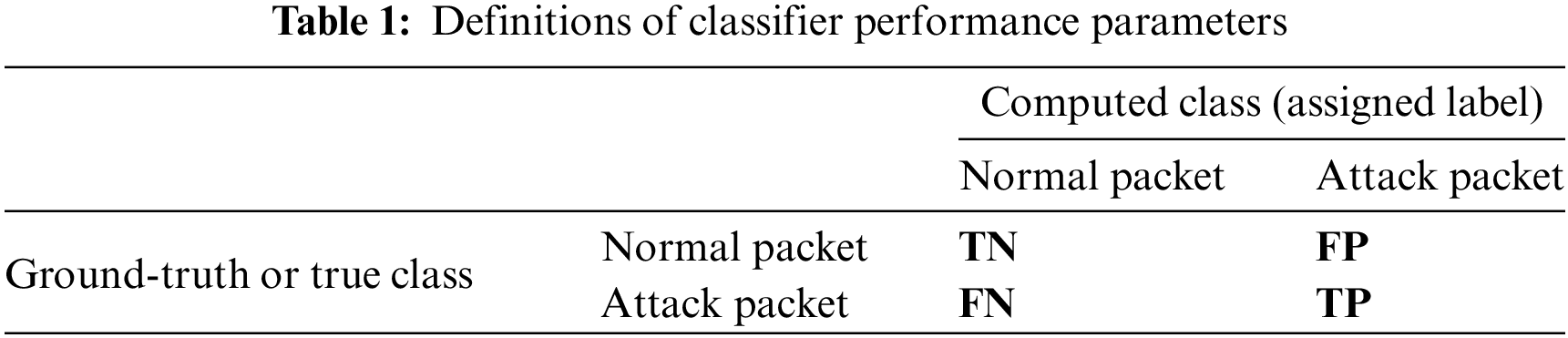
The true-positive rate (TPR) and the true-negative rate (TNR) denote, respectively, the percentage of attack and normal packets in the test set that are correctly labeled by the NN classifier. The false-positive rate (FPR) and the false-negative rate (FNR) denote, respectively, the percentage of normal and attack packets that are misclassified. The additional classifier performance parameters that are used in this report include classifier precision, recall, and F-score. The classifier precision denotes the true-positive rate (TPR) divided by the total number of test packets that are classified as attack packets by the classifier. The classifier recall is the true-positive rate (TPR) divided by the total number of attack packets in the test set. The classifier F-score is the harmonic mean of its precision and recall.

precision=TPRTPR+FPR.(27a)

recall=TPRTPR+FNR.(27b)

F−score=2×precision×recallprecision+recall.(27c)

The plots of Fig. 6 show the effect of the number of trainers on the classifier performance as measured by the five metrics defined above. Here, the classifier, in addition to the input and output layers, is comprised of one hidden layer with ten nodes. The number of test packets was set at two thousand, equally divided between normal and attack packets. None of the training packets were included in the test set, and the NN was trained using ten epochs with a batch size of one, namely, stochastic gradient descent training. For each setting of the number of trainers, the experiment was repeated twenty-five times, and the performance results were averaged across all the trials of the experiment.

Figure 6: Effect of number of trainers on performance of classifier with one hidden layer

The box plots of Fig. 7 show the distributions of the true-positive rate and the true-negative rate across twenty-five instantiations of the experiment. The plots of Figs. 6 and 7 show that as the number of normal and attack trainers increases from ten to one hundred, the classifier performance improves as expected. This experiment shows that an FFNN classifier with one hidden layer comprising ten nodes, trained with two hundred packets equally divided between normal and attack, leads to precision exceeding 99.7%, which is a remarkable achievement. The plots of Fig. 7 also show that as the number of trainers increases, the statistical dispersion of the classifier performance parameters, namely, TPR and TNR, tightens across different instantiations of the experiment.

Figure 7: Effect of the number of trainers on distributions of TPR and TNR of the classifier with one hidden layer

The plots of Fig. 8 show the effect of the number of trainers on the performance of classifiers with different numbers of hidden layers. In these experiments, three different FFNN classifiers, namely, with one, two, and three hidden layers, were trained, and the performance of each trained classifier was assessed. Each classifier has ten nodes in each of its hidden layers. The numbers of normal and attack packets used in the training sets of different classifiers varied from one hundred to one thousand. As expected, as the number of trainers increases, the classifier’s performance improves. The plot in the fourth quadrant of Fig. 8 shows that increasing the number of hidden layers does not appreciably improve the classifier performance, as measured by the F-score. The plots of Figs. 9 and 10 show the effect of the number of nodes in the hidden layer on the performance of a classifier with one hidden layer. The number of trainers from normal and attack classes was fixed at twenty, and two thousand test packets were equally divided between normal and attack packets. For each setting of the number of nodes, the experiment was repeated one hundred times, and the performance results were averaged across all the instantiations of the experiment. It is seen from Fig. 9 that performance, as measured by the F-score of the classifier, improves as the number of nodes increases from one to ten, where it reaches a plateau. Increasing the number of nodes beyond ten does not have an appreciable effect on the performance, as measured by the F-score. The plots of Fig. 10 show the distributions of true-positive and true-negative rates across all the one hundred instantiations of the experiment. As the number of nodes increases, there seems to be a tightening of the true negative rate, as shown by the box plot on the right of Fig. 10. This shows that the greater number of nodes improves the performance, as measured by the worst-performing classifier in the one hundred instantiations of the classifier in this experiment.

Figure 8: Effect of number of trainers on the performance of classifiers with different number of hidden layers

Figure 9: Effect of number of nodes of hidden layer on classifier performance

Figure 10: Effect of number of nodes of hidden layer on TPR and TNR distributions

This study compared the performance of three classifiers: a binary neural network (NN) with one hidden layer of ten nodes, a k-nearest neighbors (KNN) classifier with three neighbors, and a support vector classifier (SVC) with a linear kernel. All three machine learning algorithms were implemented using the Scikit-learn library. The classifiers were trained on the same data and evaluated on an identical test set consisting of 1000 packet headers from each class in the KDD dataset. For each setting of the number of trainers each experiment was repeated 100 times using randomly selected trainers, and the average performance across all repetitions is reported in Table 2. Among the three classifiers compared, the neural network (NN) demonstrated the highest performance for binary classification of network traffic packets, exceeding the k-nearest neighbor (KNN) and support vector classifier (SVC).

9  Conclusions

This paper establishes the mathematical underpinnings of the fully connected feedforward neural network (FFNN), commonly known as the multi-layer perceptron (MLP), and elucidates the intricate formulations of the backpropagation and gradient descent algorithms employed for adjusting network weights and biases throughout the training phase. Comprehensive derivations of the mathematical formulas delineating the forward propagation from the input to the output of the neural network (NN) are presented, alongside an analysis of its computational complexity. The NN is applied to conduct a binary classification of network traffic utilizing a well-known open-source benchmark dataset. The paper evaluates the impact of different parameters, including network configurations such as the number of hidden layers and the number of nodes within each hidden layer, as well as the number of trainers, on the performance of the classifier. The statistical distributions of the true-positive and true-negative rates of the classifier are analyzed across various experimental setups, which involve random selection of training and testing elements under different scenarios including variations in the number of hidden layers and nodes. Compared to the k-nearest neighbor (KNN) and support vector classifier (SVC), the study demonstrates that a neural network (NN) classifier achieves superior accuracy in binary classification of network traffic packets.

Acknowledgement: None.

Funding Statement: Kaveh Heidary’s research project was partially funded by Quantum Research International Inc. through Contract QRI-SC-20-105. https://www.quantum-intl.com/.

Availability of Data and Materials: The network traffic data used in this paper is open-source and can be downloaded from the following source: https://kdd.ics.uci.edu/databases/kddcup99/kddcup99.html (accessed on 08/04/2024).

Conflicts of Interest: The author declares that they have no conflicts of interest to report regarding the present study.

References

1. M. G. Solomon and D. Kim, “Evolution of communication technologies,” in Fundamentals of Communications and Networking, 3rd ed. Burlington MA, USA: Jones & Bartlett Learning, 2022, pp. 1–26. [Google Scholar]

2. B. A. Forouzan, “Network layer: Delivery, forwarding, and routing,” in Data Communication and Networking with TCP/IP Protocol Suite, 6th ed. New York, NY, USA: McGraw Hill, 2022, pp. 647–699. [Google Scholar]

3. P. Baltzan and A. Phillips, “Databases and data warehouses,” in Essentials of Business Driven Information Systems, 5th ed. New York, NY, USA: McGraw Hill, 2018, pp. 169–208. [Google Scholar]

4. National Institute of Standards and Technology (NISTGuide to Operational Technology (OT) Security, NIST SP 800-82, Rev 3, Sep. 2023. Accessed: Apr. 5, 2024. [Online]. Available: https://nvlpubs.nist.gov/nistpubs/SpecialPublications/NIST.SP.800-82r3.pdf [Google Scholar]

5. “The White House National cybersecurity strategy,” Mar. 2023. Accessed: Apr. 8, 2024. [Online]. Available: https://www.whitehouse.gov/wp-content/uploads/2023/03/National-Cybersecurity-Strategy-2023.pdf [Google Scholar]

6. L. Atzori, A. Iera, and G. Morabito, “The internet of things: A survey,” Comput. Netw., vol. 54, no. 15, pp. 2787–2805, Oct. 2010. doi: 10.1016/j.comnet.2010.05.010. [Google Scholar] [CrossRef]

7. M. Ammar, G. Russello, and B. Crispo, “Internet of things: A survey on the security of IoT frameworks,” J. Inf. Secur. Appl., vol. 38, pp. 8–27, Feb. 2018. doi: 10.1016/j.jisa.2017.11.002. [Google Scholar] [CrossRef]

8. L. Chen, S. Tang, V. Balasubramanian, J. Xia, F. Zhou and L. Fan, “Physical-layer security based mobile edge computing for emerging cyber physical systems,” Comput. Commun., vol. 194, pp. 180–188, Oct. 2022. doi: 10.1016/j.comcom.2022.07.037. [Google Scholar] [CrossRef]

9. R. W. Lucky and J. Eisenberg, “National Academies Renewing U.S. telecommunications research,” in National Research Council of the National Academies, Committee on Telecommunications Research and Development. Washington, DC, 2006. Accessed: Nov. 10, 2023. [Online]. Available: http://www.nap.edu/catalog/11711/renewing-us-telecommunications-research [Google Scholar]

10. Y. Li and Q. Liu, “A comprehensive review study of cyber-attacks and cyber security: Emerging trends and recent developments,” Energy Rep., vol. 7, pp. 8176–8186, Nov. 2021. doi: 10.1016/j.egyr.2021.08.126. [Google Scholar] [CrossRef]

11. S. Ansari, S. G. Rajeev, and H. S. Chandrashekar, “Packet sniffing: A brief introduction,” IEEE Potentials, vol. 21, no. 5, pp. 17–19, 2003. doi: 10.1109/MP.2002.1166620. [Google Scholar] [CrossRef]

12. M. A. Qadeer, A. Iqbal, M. Zaheed, and M. R. Siddiqi, “Network traffic analysis and intrusion detection using packet sniffer,” in 2010 Second Int. Conf. Commun. Softw. Netw., Singapore, 2010, pp. 313–317. doi: 10.1109/ICCSN.2010.104. [Google Scholar] [CrossRef]

13. K. E. Hemsly and R. E. Fisher, “History of industrial control system cyber incidents,” in Idaho National Laboratory Report, US Department of Energy, Dec. 2018. [Google Scholar]

14. P. Gupta and V. McKeown, “Algorithms for packet classification,” IEEE Network, vol. 15, pp. 24–32, 2001. Accessed: Jan. 15, 2024. [Online]. Available: https://cse.sc.edu/~srihari/reflib/GuptaIN01.pdf [Google Scholar]

15. C. L. Hsieh, N. Weng, and W. Wei, “Scalable many-field packet classification for traffic steering in SDN switches,” IEEE Trans. Netw. Serv. Manag., vol. 16, no. 1, pp. 348–361, Mar. 2019. doi: 10.1109/TNSM.2018.2869403. [Google Scholar] [CrossRef]

16. A. S. Qureshi, A. Khan, N. Shamin, and M. H. Durad, “Intrusion detection using deep sparse auto-encoder and self-taught learning,” Neural Comput. Appl., vol. 32, no. 8, pp. 3135–3147, Apr. 2020. doi: 10.1007/s00521-019-04152-6. [Google Scholar] [CrossRef]

17. D. Ding, Q. L. Han, Y. Xiang, A. Ge, and X. M. Zhang, “A survey on security control and attack detection for industrial cyber-physical systems,” Neurocomputing, vol. 275, pp. 1674–1683, Jan. 2018. doi: 10.1016/j.neucom.2017.10.009. [Google Scholar] [CrossRef]

18. R. Alguliyev, Y. Imamverdiyev, and L. Sukhostat, “Cyber-physical systems and their security issues,” Comput. Ind., vol. 100, pp. 212–223, Sep. 2018. doi: 10.1016/j.compind.2018.04.017. [Google Scholar] [CrossRef]

19. V. P. Janeja, “Understanding sources of cybersecurity data,” in Data Analytics for Cybersecurity. Cambridge, UK: Cambridge University Press, 2022, pp. 14–27. [Google Scholar]

20. I. H. Sarker, A. S. M. Kayes, S. Badsha, H. Alqahtani, P. Watters and A. Ng, “Cybersecurity data science: An overview from machine learning perspective,” J. Big Data, vol. 7, no. 41, pp. 1–29, Jul. 2020. [Google Scholar]

21. I. Goodfellows, Y. Bengio, and A. Courville, “Machine learning basics,” in Deep Learning. Boston, MA, USA: MIT Press, 2016, pp. 98–155. [Google Scholar]

22. C. C. Aggarwall, “Deep learning: Principles and learning algorithms,” in Neural Network and Deep Learning: A Textbook, 2nd ed. Yorktown Heights, NY, USA: Springer, 2021, pp. 119–162. [Google Scholar]

23. D. H. Ackley, G. E. Hinton, and T. J. Sejnowski, “A learning algorithm for Boltzmann machines,” Cogn. Sci., vol. 9, pp. 147–169, Jan. 1985. doi: 10.1207/s15516709cog0901_7. [Google Scholar] [CrossRef]

24. Y. Bengio, “Deep learning of representations: Looking forward,” in Proc. First Int. Conf. Stat. Lang. Speech Process., Berlin, Heidelberg, Springer, May 2013, vol. 7978. doi: 10.1007/978-3-642-39593-2_1. [Google Scholar] [CrossRef]

25. Y. LeCun, Y. Bengio, and G. E. Hinton, “Deep learning,” Nature, vol. 521, pp. 436–444, May 2015. doi: 10.1038/nature14539. [Google Scholar] [PubMed] [CrossRef]

26. G. E. Hinton and R. R. Salakhutdinov, “Reducing the dimensionality of data with neural networks,” Science, vol. 313, no. 7586, pp. 504–507, Jul. 2006. doi: 10.1126/science.1127647. [Google Scholar] [PubMed] [CrossRef]

27. A. Ardakani, F. Leduc-Primeau, N. Onizawa, T. Hanyu, and W. J. Gross, “VLSI implementation of deep neural networks using integral stochastic computing,” IEEE Trans. Very Large Integr. (VLSI) Syst., vol. 25, no. 10, pp. 2688–2699, Oct. 2017. doi: 10.1109/TVLSI.2017.2654298. [Google Scholar] [CrossRef]

28. L. Alzubaidi et al., “Review of deep learning: Concepts, CNN architectures, challenges, applications, future directions,” J. Big Data, vol. 8, no. 53, pp. 1–74, Mar. 2021. doi: 10.1186/s40537-021-00444-8. [Google Scholar] [PubMed] [CrossRef]