Distributed Federated Split Learning Based Intrusion Detection System

1  Introduction

The Internet of Things (IoT) is the most important technology, and it has grown exponentially. IoT is a set of technologies that connect a wide range of IoT devices and generate a large volume of data with features of larger size, higher velocity, and heterogeneity [1]. At the same time, the evolution of 5G networks has given strength to the growth of the IoT. 5G is characterized by higher capacity and lower latency to facilitate communication of billions of devices over the Internet. Therefore, the 5G network should be integrated with modern technologies to provide exceptional services [2]. One of the important 5G-enabling technologies is Multiple-Input-Multiple-Output (MIMO), which has been used in recent years to provide high spectral efficiency and high throughput [3].

The growth of 5G-based IoT (5G-IoT) comes with challenges related to IoT data, such as security and privacy, and they also have an impact on computational complexity and cost in data storage and data processing. An important IoT domain that needs 5G features in transmission and channel utilization is the Internet of Medical Things (IoMT) [4]. The IoMT is a latency-sensitive application expected to be deployed based on 5G technologies. It will have a great role in maintaining the sustainability of smart cities [5]. Fig. 1 describes the 5G-IoMT architecture, including three layers: sensing layer, fog computing layer, and cloud computing layer. First, the data is collected using various sensors or medical devices in the sensing layer. These devices are resource-constrained and have low computation power. The data is passed to the fog computing layer via communication protocols, where more powerful computing fog servers process it to avoid latency. The data is transmitted in the 5G structure through multiple Base Stations (BSs) that employ fog computing. Finally, the data is transmitted from the fog computing layer to the cloud computing layer to store and update the patient’s data [6].

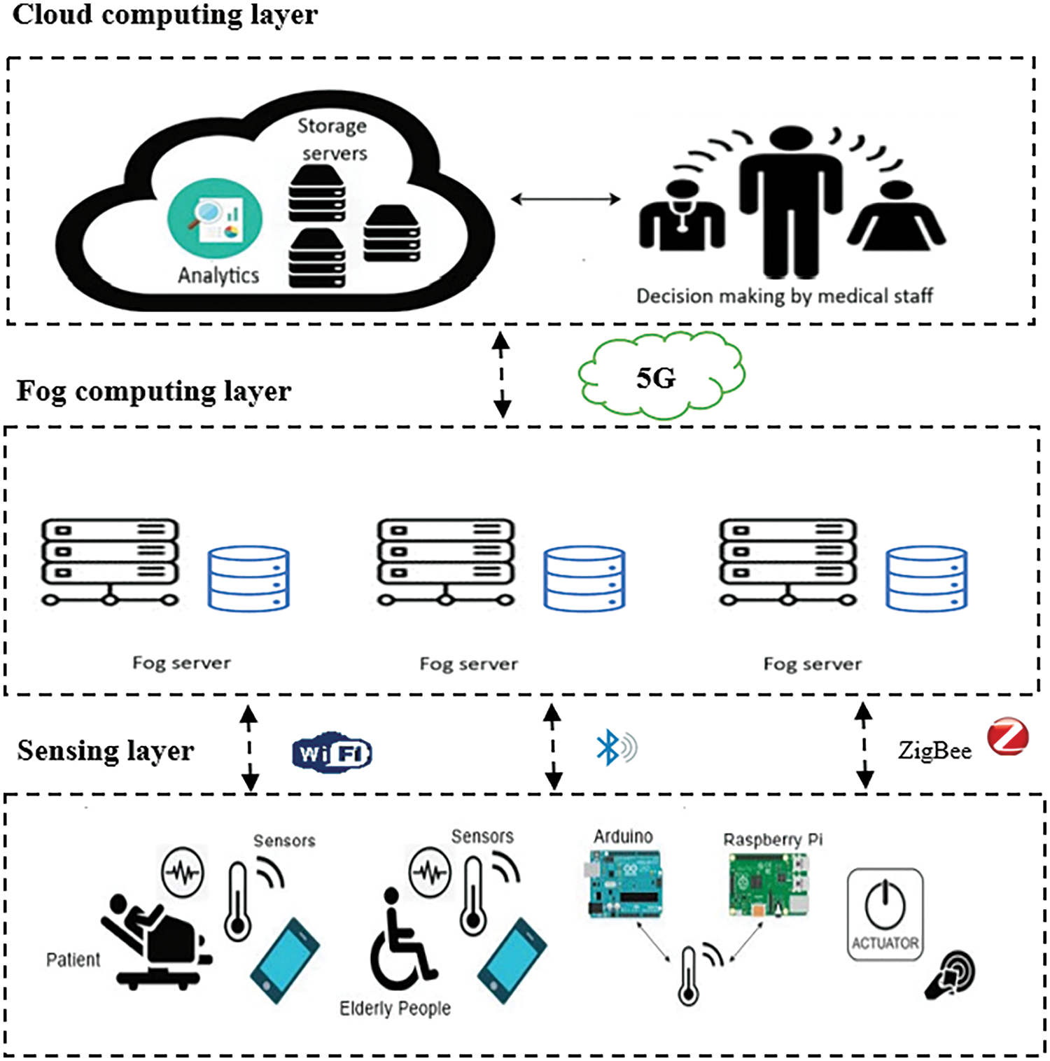
Figure 1: 5G-IoMT system architecture

The significant increase in transmitting a large volume of data across distributed networks makes security one of the most important challenges in IoMT. Recently, Distributed Denial of Service (DDoS) attacks have increased dramatically, leading to significant consequences [7]. One of the most popular real examples of DDoS against medical institutions was in 2016 when the attacker used malware to breach the Banner Health network in Arizona and access the patient’s information, including patient’s social numbers, dates of services, and information related to the insurance. The attack went undetected for a month, with 3.7 million patients affected. It cost $1.25 million to resolve the data breach issue [8].

Intrusion Detection Systems (IDSs) based on the Centralized Learning (CL) approach are widely used to detect security attacks. CL is a traditional learning approach where the data is uploaded from each connected client device to the cloud server to train the entire model and distribute it to all devices [9]. IDSs using Machine Learning (ML) methods are impractical in the new network environment, and they are not effective in detecting attacks in massive and distributed environments. Although centralized systems based on Deep Learning (DL) achieve acceptable accuracy, they include limitations such as connectivity, bandwidth, latency, communication overhead, computation power, and distributed data security. In addition, it is not scalable to the size of IoMT [10].

IDSs based on distributed learning, such as Federated Learning (FL) or Split Learning (SL), are used in distributed environments to overcome the limitations of CL. FL is an efficient approach that trains the model with its local data among multiple clients and shares the model update with the server. FL preserves data privacy while enabling collaborative model development. However, FL suffers from high training time and communication overhead [11]. On the other hand, SL splits the model into two parts, one for clients and one for servers, which reduces the computational cost and can help reduce training time [12]. SL offers advantages in terms of computational resources, but it faces challenges such as communication overhead and potential security vulnerabilities at the split point. Both FL and SL are not efficient when the number of clients increases, having heterogeneous datasets, and with constraints on communication resources. Federated Split Learning (FSL) is emerging research combining FL and SL that could solve problems of both FL and SL and offer more secure, efficient, and scalable distribution systems [13]. Most existing IDSs are not scalable to the network size. It suffers from low detection accuracy, training time, and communication overhead. These issues have negatively affected the throughput of real-time applications such as IoMT, and we need to solve them urgently.

Recently, a user selection strategy has been used to reduce communication overheads. In FL, different selection schemes have been proposed in [14], including four schemes. The first scheme is Best Channel (BC), where the user is selected based only on the channel condition. The second scheme is Best l2-Norm (BN2), where the user is selected according to the significance of the model update. The third scheme is Best Channel-Best l2-Norm (BC-BN2), which considers the channel condition and the significance of the model update. The last scheme is Best l2-Norm-Channel (BN2-C), where each user performs a Decentralized Stochastic Gradient Descent (D-SGD) quantization scheme assuming all bandwidth availability to itself and finds the resultant quantized vector and the significant importance of the local update is sent to the server. In [15], a user equipment UE selection scheme named Multi-Arm Bound (MAB) is based on BC-BN2 (MAB-BC-BN2). The proposed scheme uses the discounted Upper Confidence Bound (UCB) strategy to make the selection decision based on the UCB score. Nevertheless, the above schemes, including channel quality and the importance of local model update, are popular selection strategies in FL. In practice, it is not practical because it is difficult to get an accurate selection before the learning process is executed, which leads to more computation and communication consumption.

Motivated by the above, this paper proposed a distributed FSL (DFSL) system to detect DDoS attacks, enhancing detection accuracy and reducing training time and communication overhead. Three research questions were formulated as follows:

Q1: How do we distribute the detection model with high detection accuracy and low training time?

Q2: How can the communication overhead of the system be reduced?

Q3: How can we test the effectiveness of the proposed system?

To address the research questions of this paper, the following contributions were identified:

1.    Propose a novel distributed FSL (DFSL) system to detect DDoS attacks in IoMT. An adaptive aggregation method is designed based on the early stopping strategy to reduce training time and enhance detection accuracy.

2.    Propose a Multi-Node Selection (MNS) based Best Channel-Best l2-Norm (BC-BN2) selection scheme to reduce communication overhead. The nodes are selected based on the importance of local update, channel quality, and the nearest distance from the server. The MNS dynamically identifies the irrelevant local updates during the training process to avoid computation and communication resources consuming.

3.    Test the system performance using Convolutional Neural Network (CNN) and a hybrid model that combines the CNN and long Short-Term Memory (LSTM), on two modern datasets such as CICDDoS2019 and LITNET-2020, and compare the performance with baseline distributed approaches such as FedAvg, Vanilla SL, and SplitFed algorithms.

The paper is organized as follows. A brief overview of FL, SL, FSL, and related works is provided in Section 2. Section 3 describes the problem formulation. The proposed work of the DFSL system and MNS scheme are described in Section 4. Section 5 describes the dataset description and data preprocessing. The performance results and comparative analysis are presented in Section 6. The discussion is presented in Section 7. Finally, the conclusion and future work is described in Section 8.

2  Literature Review

This section described a background for the FL, SL, and FSL approaches. Then, related works that are based on ML, CL, and distributed learning IDS in IoMT networks are presented.

2.1 Federated Learning

In Federated Learning (FL) [16], the model is trained at each client in parallel with its local data for its local epochs. After that, the local model updates are sent to the server for model aggregation. The server aggregates the received local updates, generates the global model update, and sends it back to the clients so they can train for the next round. After receiving the global model update, each client trains the global parameters on its local data and sends its local update to the server. This process continues until the model converges. Federated Averaging (FedAvg) algorithm [17] is the popular centralized aggregation algorithm in FL. FedAvg algorithm considers a weighted average of the gradients for the model updates. Based on the FedAvg procedure, as shown in Fig. 2, the server initializes the global model parameter w0 and broadcasts the initial global parameter to the clients. Then, each client n receives the initial parameter and starts the local training with its local data Dn. The local loss function L for each client n with Dn is calculated as

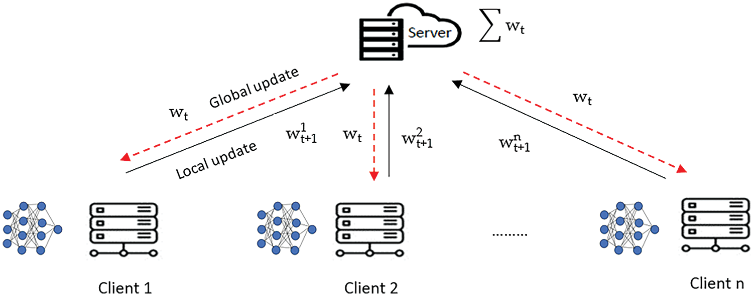
Figure 2: FedAvg architecture

Ln(w)=1|Dn|∑i∈Dnl(w,sni)(1)

where |Dn| is the dataset size and l(w,sni) is the loss function of the model at data sample sni. The global loss function L(w) over the data for the clients is calculated as

L(w)=∑n=1NDnLn(w)D(2)

where D is the global data, and N is the number of clients. The local training updates wt+1n is calculated as

wt+1n=wtn−αt∇g(wtn)(3)

where αt is the learning rate, ∇g(wtn) is the gradients for wtn of loss function L. The global model parameter wt is updated at the server by aggregating each local update wt+1n from each client and sending it back to the clients; this process is repeated until the loss function reaches the optimal value for the global model. The global model update is represented as

wt=∑n=1NDnwt+1nD(4)

2.2 Split Learning

In Split Learning (SL), the model is trained sequentially with its local data. The training raw data is stored in the client, and the server cannot access the raw data. Four SL configuration strategies include Vanilla SL, U-shaped SL, Vertically SL, and two-part SL configurations. Vanilla SL [18] is the most popular SL algorithm where the model is partitioned into at least two parts and shares labels. The first part runs on the client wt+1n, and the second part runs on the server wts; it trains its smashed data up to the cut layer C, as shown in Fig. 3. Each client needs to update its local model parameters before starting the next round of training. In the sequential training, the client performs forward propagation wt+1n on its local data Dn and sends the activations atn up to the cut layer to the server. Then, the server receives the client’s activation atn and performs the forward propagation until the last layer of the model wts. After that, the server performs the backpropagation, and the gradient gtn of the client cut layer is sent back to the client. Then, the client updates the model on its side and sends it back to the server for updates.

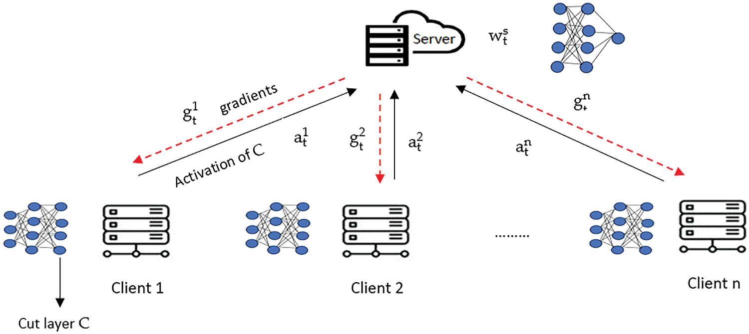
Figure 3: Vanilla SL architecture

U-shaped SL is another split configuration similar to Vanilla SL but without label sharing. Because the client does not share the label, the client completes learning. In U-shaped SL, the client has one or more bottom layers and one or two top layers, whereas the middle layers are allocated by the server. Vertically SL is a way to train a split model with different data without sharing data. Each client trains a part of the model up to the cut layer C. After that, the data is sent to the server to complete the rest of the learning process. Finally, two-part SL is a strategy to split the model into only two parts between clients and server [19]. The SL helps reduce training time where the model is portioned among multiple clients and server, but most of the SL algorithms suffer from high communication overhead.

2.3 Federated Split Learning

Federated Split Learning (FSL) is a promising distributed learning that combines FL and SL approaches and takes advantage of the two approaches. It trains the model in parallel among multiple distributed clients in FL and splits the entire model between the clients and server in SL. SplitFed is the first method in FSL that eliminates the drawbacks of FL and SL. Unlike FL, the model is portioned and trained among the clients and the server to reduce training time. On the other hand, it does their training in parallel to reduce computation time and enhance learning performance, as in FL. It works similarly to the classic SL setting, except the existing fed server on the client side performs federated aggregation [20]. MiniBatch-SFL is proposed to incorporate MiniBatch SGD to FSL, where the clients train the client-side model in an FL fashion, and the server trains the server side and analyzes the convergence of the data [21]. A Communication and Storage Efficient FSL (CSE-FSL) strategy is proposed using the auxiliary network to update the local model at the client while keeping only a single model at the server, which helps to avoid the communication of gradients from the server and reduces the server resource requirement [22]. Finally, a comparison of the FL and SL settings regarding communication efficiency is explained in [23].

2.4 Related Works

The following presents the most current IDS for detecting attacks in the IoMT environment.

Saheed et al. [24] developed an efficient IDS in IoMT based on Deep Recurrent Neural Network (DRNN) and ML models such as Random Forest (RF), Decision Tree (DT), K-Nearest Neighbors (KNN), and ridge classifiers. The goal is to classify and forecast unexpected cyber-attacks. They evaluated the developed IDS with the NSL-KDD dataset, and it outperformed the existing approaches with an accuracy of 99.76%. Manimurugan et al. [25] proposed a DL-based method Deep Belief Network (DBN) algorithm for IDS in IoMT. The CICIDS2017 dataset is used to test the proposed algorithm. The results achieved 96.67% accuracy for the DoS/DDoS class, 95.21% precision, 97.34% recall, 0.97 F-measure, and 97.31% detection rate. Usman et al. [26] proposed a framework that divides an underlying wireless multimedia sensor network into many clusters in IoMT. Each cluster has a cluster head, which is responsible for protecting the privacy data via data and location coordinates aggregation. Then, the aggregated data are processed on the cloud using Artificial Neural Network (ANN). The proposed P2DCA framework is implemented with the CICIDS2017 dataset and compared with the existing schemes. It achieved 150 min training time, 350 MB communication overhead, and 95.56% accuracy. Ren et al. [27] proposed Data Optimization IDS (DO-IDS) to identify the anomaly behaviors in the network. The proposed DO-IDS used hybrid data optimization. They used Isolation Forest (iForest) in data sampling and Genetic Algorithm (GA) to optimize the sampling ratio. The RF and GA are used in feature selection to obtain the optimal subset. The DO-IDS is tested using the RF classifier with the UNSW-NB15 dataset; it scored an accuracy of 92.8% and a false alarm rate of 0.330.

Some of the studies used the CL approach to detect attacks. Gudla et al. [28] proposed a Deep Intelligent DDoS Detection Scheme (DI-ADS) for IoT applications. The model is implemented in the fog layer to predict the behavior of the fog devices. The scheme was implemented using Multilayer Perceptron (MLP) on a dataset for Software Defined System called DDoS-SDN that consists of three types of DDoS attacks. The results showed the accuracy of 97.84% and 1000 min training time. Priyadarshini et al. [29] proposed a source-based DDoS defense mechanism in fog and cloud environments. The defender module is deployed at the SDN controller to detect abnormal behavior in the network and transport layer. The detection model is implemented using LSTM on CTU-13 Botnet and ISCX 2012 IDS datasets. The accuracy of the model was 87.67% and 87.96% for CTU-13 Botnet and ISCX 2012 IDS, respectively. Zhang et al. [30] proposed a DDoS detection model based on Bidirectional LSTM (BiLSTM) at edge computing. The model achieves information extraction using the BiLSTM network and automatically learns the characteristics of the attack traffic in the original data traffic. The proposed model, called power IoT, was implemented in their data and achieved an accuracy of 95%, 250 min training time, and 520 MB communication overhead.

For distributed learning, little works addresses the security in IoMT using FL, SL, and FSL approaches. Verma et al. [31] proposed an FL Deep Intrusion Detection (FLDID) framework in smart industries. The proposed framework builds a collaborative model to detect DDoS attacks. They used CNN+LSTM+MLP in the detection model with the X-IIoTID dataset. The proposed framework outperforms the other approaches with 99.22% accuracy and 3042 s training time. Rey et al. [32] proposed an FL framework to detect malware in IoT devices. The N-BaIoT dataset is used and is designed for network traffic of multiple IoT devices. Two different DL models, MLP and Autoencoders (EA), are used for detection. The performance of the models is compared with the traditional approach, which shares its data with the server, and with the traditional approach, which does not share its data. The performance of the proposed framework scored an accuracy of 95% and 88 MB communication overhead. Alhasawi et al. [33] introduced a federated learning-based approach to detect DDoS attacks known as FL for decentralized DDoS Attack Detection (FL-DAD). The detection model used CNN to effectively identify DDoS attacks on the CICIDS2017 dataset. The model is compared with centralized detection methods, and it achieved 99.3% accuracy, 48.3 s training time, and 390.2 MB communication overhead with the maximum number of nodes.

Yu et al. [34] proposed a Pseudo-Client ATack (PCAT) based on SL to detect DDoS attacks with more challenging situations where the client model is unknown to the server. They investigated the inherent privacy leakage via the server model in SL, where the server model can easily steal the data. The server trains a small part from the dataset, about 0.1%–5%, for the same learning task. The performance is evaluated using the Deep Neural Network (DNN) model on the MINIST dataset with a two-part SL strategy, where the results scored an accuracy of 96.98%. Abuadbba et al. [35] examined the SL on the 1D CNN model to detect DDoS attacks. They tested the model with medical ECG data and added two mitigation techniques. The first technique adds more hidden layers to the client side. The second technique applies various privacy. The model achieved 98% accuracy and 20 min training time.

Khan et al. [36] performed the first empirical analysis of the SplitFed algorithm. They used SplitFed to design a strong detection model. The CIFAR10 and FEMNIST datasets are used with Alexnet and VGG11 models to perform the training process. The results of the Alexnet and VGG11 in the CIFAR10 dataset, the accuracy scored 62.4% and 73%, respectively. For the custom model in the FEMNIST dataset, the accuracy scored 81%. The communication overhead scored 150 and 200 MB for both datasets. Li et al. [37] proposed an attack detection approach FSL in real IoT scenarios. The proposed approach for the construction of global models of various time series in the context of data isolation has the ability to detect attacks. The experiment is applied to the CNN model and MNIST dataset. It achieved an accuracy of 93.56%, precision of 92.78%, recall of 93.19%, and F-measure of 92.98%.

All related works that are mentioned above are summarized in Table 1.

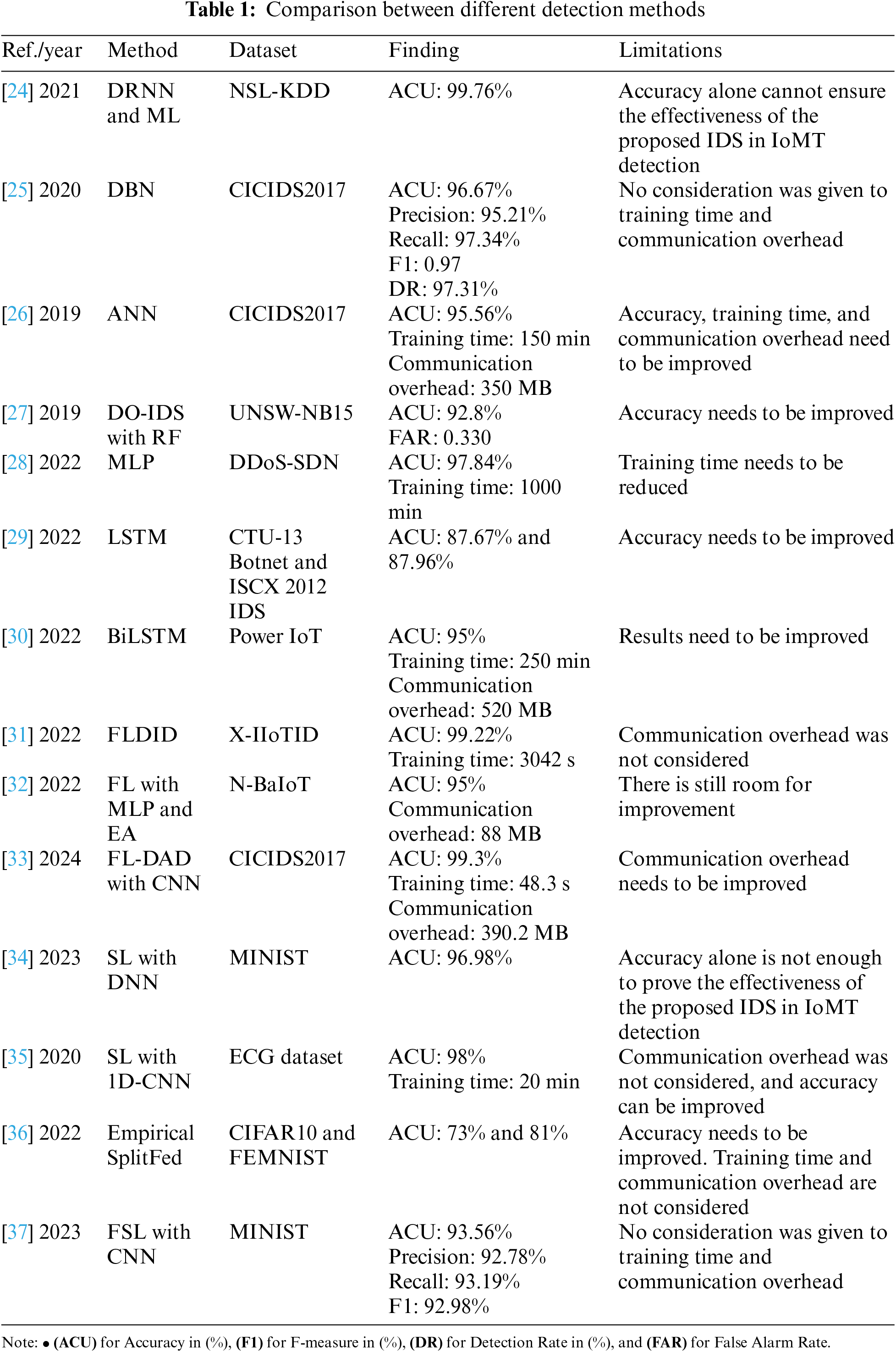
Three important criteria to improve IoMT networks are detection accuracy, latency, and communication overhead. Most existing works that address the security in IoMT based on ML, CL, and distributed learning suffer from low detection accuracy, high training time, and high communication overhead, which is not acceptable for real-time and latency-sensitive applications such as IoMT. In addition, most of the datasets are out of date and related to different types of security attacks; there is a lack of datasets related to DDoS attacks. To solve the problems of existing attack detection, we propose a distributed FSL (DFSL) system to detect DDoS attacks in the IoMT environment, supporting the existing issues. An adaptive aggregation method based on the early stopping strategy is proposed to enhance detection accuracy and reduce training time. In addition, to improve the communication overhead, we propose a Multi-Node Selection (MNS) based BC-BN2 scheme with three selection metrics. The proposed system is evaluated using two modern DDoS datasets, CICDDoS2019 and LITNET-2020.

3  Problem Formulation

As mentioned above, IDS based on ML and CL has multiple challenges, including learning performance, training time, and communication overhead. The first Optimization Problem (OP) considers the learning performance of ML and CL, which needs optimization to maximize the detection accuracy. FL helps to enhance the learning of a statistical model at the server to generate a model with high accuracy with distributed datasets among multiple clients. Therefore, the server needs to minimize the global loss function.

OP1: The first objective is to maximize detection accuracy by minimizing the global loss function L(w) in FL according to Eq. (2) which is subject to massively distributed data constraint where the global data D is stored across a large number of clients N. The objective function can be modeled as

J(w)=minDn(L(w))Subject to∑n=1NDn=D(5)

Although the FL may enhance learning performance, it suffers from high training time, which takes a long time to compute. The term computation refers to the number of training epochs/rounds ne and the number of model steps/epochs ns that are assigned for each client n. By multiplying these two values, we get the total number of steps/rounds of the model for each client. The total training time in one communication round t is calculated as

T=max(Twn+(ne×ns)×Tsn)(6)

where Twn is the total time for two-way transmission between client n and server s and Tsn is the total time for the client n to complete the model steps.

OP2: The second objective is to reduce the total training time T with maximum CPU frequency constraint. The objective function can be modeled as

z=min(T)Subject toCPUmin≤CPUn≤CPUmax(7)

A distributed FSL (DFSL) system with an adaptive aggregation method based on the early stopping strategy is proposed to solve OP1 and OP2. Moreover, FSL suffers from high communication overhead, especially in SL training. For each round, the server should collect the smashed data from all clients to train the server-side model, and all clients must wait for gradients from the server to update its local model. We consider the communication overhead of client n at tth communication round can be calculated as

COtn=Btnlog2(1+PtnBtn)(8)

where Btn is the allocated bandwidth of client n at the t communication round, Ptn is the transmission power of node n at t communication round.

OP3: The last objective is to reduce communication overhead with maximum transmission power constraint. The objective function can be modeled as

u=min(COtn)Subject to0≤Ptn≤Pmax(9)

A Multi-Node Selection (MNS) based BC-BN2 selection scheme is proposed to solve OP3. The proposed selection scheme selects the nodes with three selection metrics: the importance of the local update, channel quality, and the nearest distance from the server. Only the selected nodes are used for global aggregation to reduce communication overhead.

4  Proposed Distributed FSL System

This section describes the details of the proposed distribution FSL (DFSL) system. First, the channel model is illustrated. Then, the DFSL system procedure is introduced. Then, the MNS scheme is explained. Finally, model convergence and complexity analysis are described.

4.1 Channel Model

The channel model of the proposed distributed FSL (DFSL) is based on uplink massive MIMO technology. The massive MIMO technology has been used in recent years with 5G to achieve high spectral efficiency and throughput, which is needed for IoMT networks. As shown in Fig. 4, the channel model consists of multiple clients, a base station with multiple antennas, and one server. The clients are fog nodes represented as N={n1,n2,…,ni}, where each fog node represents a fog server distributed in different areas. We assume that neither the nodes nor the server is attacked. We use a 16×16 MIMO antenna configuration where increasing the number of antennas helps avoid interference with the neighbor nodes. We suppose the uplink massive MIMO is equipped with M antennas at the base station and communicates with the set of fog nodes N simultaneously. If the signal is transmitted from the node to estimate the channel is x∈CN, it is received at the base station during uplink transmission as

Figure 4: System channel model

y=Hx+nuplink(10)

where y∈CM is the signal received, H is the channel vector between the node and base station, and elements of H∈CM×Nare independent and distributed with unit variance and zero mean H∼CN(0,1). The nuplink∈CM is the additional interference from the multiple transmission and receiver noise. This interference is independent of the node signal x, but it can be dependent on the channel H as

nuplink=nuplink−interference+nnoise(11)

4.2 DFSL Procedure

The proposed DFSL is based on the FSL approach to maximize detection accuracy and reduce training time. Fig. 5 shows the DFSL system framework. Because the IoMT devices are resource-constrained and limited in computations, our DFSL algorithm works on fog nodes which have high computation capabilities and can avoid latency in computations. The proposed system works in three phases including initialization and model splitting, local model training, and adaptive aggregation.

Figure 5: Proposed DFSL framework

4.2.1 Initialization and Model Splitting

The server randomly selects the nodes randomly and broadcasts the initial global parameter w0 to all selected nodes. After receiving the initial parameter, the model is split between the node and server. Based on the two-part SL strategy, the CNN and CNN+LSTM models are split into two parts, as shown in Fig. 6. The first part runs on the node side, and the second runs on the server side. The CNN model is used with four convolutional layers (Conv), two max-pooling layers (Max-Polling), two dropout layers (Dropout), and three fully connected layers (FC). The first part consists of Conv 1 and Conv 2 operated with (convolution filters = 16, filter size = 3, and output shape = 16 × 196 feature matrix), Max-Pooling 1 with pooling size = 2, (Conv 3 and Conv 4) operated with (convolution filters = 32, filter size = 3, and output shape = 16 × 128 feature matrix), and max-pooling 2 with pooling size = 2. The second part has many layers, including FC 1, Dropout 1, FC 2, Dropout 2, and FC 3. One padding is applied before each convolution operation, and the Rectified Linear Unit (ReLU) is chosen as an activation function of hidden layers. Sigmoid is used to activate the last FC layer. For the CNN+LSTM model, the same layers with the same configuration add an LSTM layer after Max-Pooling 2 in the part that is operated with (filter size = 64 and the output shape = 64 × 128).

Figure 6: Two-part SL (a) CNN; (b) CNN+LSTM

4.2.2 Local Model Training

After model splitting, each node with its smashed data computes activation atn up to its cut layer C with the server and updates its local model update. Now, the server receives the atn and performs the forward propagation ats from its split layer up to the last layer in the model and calculates the loss function Ln(wt+1n). After that, the backpropagation is calculated and sent back to the node to update its model part. When the server receives the final update from the node, it calculates the backpropagation to the last layer and updates the model wt+1n. The backpropagation (gradient) and model update on the server side are calculated as

gts=∇L(ats,wts)(12)

gtn=∇L(atn,wtn)(13)

The local model updates on the node side are calculated as

wt+1n=wtn−αt∇g(wtn)(14)

4.2.3 Adaptive Aggregation

An adaptive aggregation method is proposed to reduce training time and enhance detection accuracy. When training a model, the weights are the most important parameter for learning the model. The objective of the nodes’ local training process is to find the weight that enhances the global model’s accuracy on the local training sets. Therefore, the proposed adaptive aggregation adopts a computation amount controlled strategy that performs a certain number of model training steps per round to each node. This controlled strategy is based on the gap between the current local model’s accuracy and loss on the training set, as well as the maximum achievable accuracy and minimum achievable loss.

Unlike FedAvg, which perform fixed computation (ne and ns) to the nodes in each communication round. The proposed adaptive aggregation method can assign specific computation amounts to each node based on the early stopping strategy. The early stopping strategy aims to prevent the training at the inflection point where the performance is not improved, reducing the overall training time. The early stopping strategy stops the training based on the classification score to enhance detection accuracy. This classification score includes the accuracy and loss scores. Accuracy and loss are important parameters that determine the model’s behavior based on its score value. As a result, nodes with larger accuracy and loss gaps are needed to perform extra training rounds to obtain the optimal score. Conversely, nodes with smaller gaps are assigned fewer steps.

Our idea is that FedAvg’s convergence can be improved by using the max score of accuracy and loss in the training set to smartly stop the training at a certain point and to set the values for ne and ns for each node and each round. By reducing the computational time, the convergence time will be optimized.

The adaptive aggregation works in three steps. First, the server determines the maximum score scoremax by computing the training accuracy for the local update at each round. Then, the accuracy value is subtracted from (μ×loss) as

scoremax=wt+1n(acc)−wt+1n(μ×loss)(15)

The μ is a hyperparameter used to balance accuracy and loss in the overall score; it is assigned to the default value μ=0.5.

Second, the current scoremax is compared to the average score scoreavg of the rest of the local updates. If the current scoremax exceeds the scoreavg value, the model is saved as best model wt+1n and the new score as best score scoreb_max. Otherwise, it will not be saved as the best model. This can be expressed as

wt+1n={w¯t+1nifscoremax >scoreavgwt+1nifscoremax <scoreavg(16)

Finally, the stopping counter sc is set to 0 when assigning the best model. Otherwise, sc is increased by one to record no improvement. When sc>patience (patience is the number of epochs/rounds with no improvements after which training will be stopped; we set the patience=10 rounds), the process stops, and the local update is starting aggregation.

Subsequently, the server aggregates the selected local updates to obtain the global model updates. The global model aggregation is calculated as

wt=wt−∑n=1n∇Ln(w¯tn)(17)

The workflow of the proposed DFSL system is described in Algorithm 1.

4.3 Multi-Node Selection

The fog nodes are connected to a wireless network via a radio communication link with constrained bandwidth. Although the DFSL reduces communication overhead by sharing model parameters rather than raw training data, the transmission of complex models from many nodes still generates much traffic. The goal is to reduce the number of nodes participating in each communication round to reduce overall communication overhead. One common technique to reduce the communication overhead in a distributed network is the node selection technique.

Based on the BC-BN2 which selects the nodes based on two metrics including the importance of local update and channel quality, the proposed MNS scheme selects the nodes based on three metrics. These metrics include the importance of local update, channel quality, and the nearest distance from the server. Selecting nodes with important local update helps to improve the model performance and get an accurate model. On the other hand, selecting the node with good channel quality and the nearest distance from the server improves communication and reduces communication time consumption.

For selecting nodes with the importance of local update, the nodes need to compare their local updates with the global update to determine the importance of its update in each communication round. The issue here is we cannot know if the global update is relevant or not until all local updates are aggregated. So, we can use the previous global update for comparison. To ensure the correct relevance between the previous global update and the current local update, we take the difference between two sequential global updates because the model training does not always have constant model convergence in each communication round. The normalized difference between two previous sequential global updates is measured as

Δwt=‖wt−1−wt‖‖wt‖(18)

where ‖⋅‖ is the Euclidean norm for a given vector, wt and wt−1 are two previous sequential global updates generated in rounds t and t−1, respectively.

A larger normalized difference means a larger divergence between the two updates. To ensure no large divergence between the two updates, the CNN and CNN+LSTM models are trained and measured for the cumulative distribution of the normalized divergence of the two global updates. As shown in Fig. 7, we see that for CNN, more than 98% of the difference is less than 0.3, where the maximum difference is 0.5. For CNN+LSTM, more than 99% has a difference of less than 0.2, where the maximum difference is 0.4. We can ensure that the previous global update can be used for the current global update. This prediction does not require more communications because each node maintains the global update made in the previous round. The current local update is compared to the previous round’s global update. The relevance between the local and global update is determined by computing the number of parameters with the same sign (gradients) in the two updates and normalizing the result by the total number of parameters. The relevance between the two updates is formulated as

r(wt+1n,Δwt)={1ifsign(wt+1n)=sign(Δwt)0Otherwise(19)

where wt+1n and Δwt are the current local update and relevant global update, respectively. If r(wt+1n,Δwt)=1, this means the wt+1n and Δwt have the same parameters sign. If r(wt+1n,Δwt)=0, this means the wt+1n and Δwt have different parameter signs.

Figure 7: Cumulative distribution of CNN and CNN+LSTM

Now, the nodes that have the important local update are denoted as N¯={n¯1,n¯2,…,n¯i}. After determining the nodes with the important local update, each relevant node n¯ is measured in its channel quality. Unlike the BC-BN2, which uses the channel gain to test the channel quality, our MNS measures the channel quality by its capacity. The channel capacity in IoMT is very important to avoid latency. The channel capacity in MIMO communication is calculated based on the Shannon theorem as

Capacity=Blog2(1+SNR)(20)

where B is the bandwidth of the channel, and SNR is the Signal-to-Noise Ratio.

When the SNR is close to 0, the term (1+SNR) is close to 1, and the logarithm term log2⁡(1+SNR) is close to 0. As a result, the Capacity is also close to 0 bps, regardless of the available bandwidth B. This means that on an extremely noisy channel with an SNR close to 0, the channel capacity is effectively zero. No meaningful information can be transmitted through the channel due to the overwhelming noise. The channel is essentially unusable for reliable data transmission. Therefore, node n¯ that has Capacity≥1 is considered good channel quality and starts to measure its distance from the server.

The nearest distance between the node n¯ and server s is determined using the K-Nearest Neighbor (KNN) algorithm. The KNN algorithm works in three steps. First, select the value of k, which represents the number of nearest neighbors that need to be considered. It differs based on the total number of nodes. Second, calculating the distance using Euclidean distance as

dis(n¯,s)=(d(xi−xj)+d(yi−yj))2(21)

where (xi,yi) are the coordinates of the node point, (xj,yj) are the coordinates of the server point, and d is the distance between (xi,yi), and (xj,yj) in a two-dimensional plane.

Finally, finding the nearest neighbor nodes, the k points with the smallest distance to the server are the nearest neighbors.

Because the first round doesn’t have a previous global update, the nodes are selected randomly. The proposed algorithm starts from the second round, only node n¯ with good channel quality and the nearest distance from the server is selected for aggregation. The procedure of the MNS scheme is described in Algorithm 2.

4.4 Convergence Analysis

In this section, the fundamental convergence analysis that affects the node side and server side on its training is performed. First, the technical assumptions are made. Then, the convergence result is presented.

A. Assumptions

First, we make the following four assumptions for convergence analysis.

Assumption 1. (ℓ-smooth) Each local loss function Ln(w) is differentiable and ℓ-smooth. For all w and w∗, we have

Ln(w)≤Ln(w∗)+(∇Ln(w∗),w−w∗)+l2‖w−w∗‖2(22)

Assumption 2. (μ-strongly convex). Let L1,…,Ln are μ-strongly convex. For all w and w∗

Ln(w)≥Ln(w∗)+(∇Ln(w∗),w−w∗)+μ2‖w−w∗‖2(23)

Assumption 3. (Unbiased and bounded stochastic gradient with bounded variance). Let ξtn represent the random sample dataset from node n, and gn(wtn) of Ln(wtn) ae unbiased with the variance bounded by σn2 that measures the level of stochasticity

Eξtn∈Dn‖gn(wtn,ξtn)−∇Ln(wtn)‖2≤σn2(24)

Further, the expected squared norm is bounded by G2

Eξtn∈Dn‖gn(wtn,ξtn)‖2≤G2(25)

Assumption 4. (Partial participation). As discussed before, only subset of nodes is selected to participate in model aggregation in each communication round t. Let N¯ be the selected subset of nodes. The probability of each node n to be selected for model aggregation is P=N¯N. Assuming the data is balanced and non-IID, thus the model aggregation at the server is represented as

wt=wt−N¯N∑n=1n∇Ln(wtn)(26)

B. Convergence result

Based on the previous assumptions, the following results are obtained.

Theorem 1. Based on Assumptions 1–4, we assume ϱ=2μ with ι=4ℓμ and N=ℓμ, then, the DFSL algorithm with N¯ nodes selected for participation satisfies

E[L(wT)]−L∗≤Nι+T−1ł(2Wμ+μι2E‖w−w∗‖2)(27)

where W=∑n=1Nσn2+6l+8G2(1−N¯N)

Proof. By defining ∇Ln=E‖w−w∗‖2 and setting ∇Ln≤wι+t with ϱ2μ and ι>0, we have

w=max{ϱ2Wϱμ−1,(ι+1)E‖w1−w∗‖}(28)

≤ϱ2Wϱμ−1,(ι+1)E‖w1−w∗‖

≤4Wμ2,(ι+1)E‖w1−w∗‖

Then by ℓ-smooth of L(⋅) and let N=ιμ,

E[L(wt)]−L∗≤ι2∇t≤ι2W2t+ι≤Nt+ι(2Wμ+μ(ι+1)2E‖w1−w∗‖)(29)

The convergence of the model is stable without extra communication overhead. Moreover, the convergence performance doesn’t affect the number of selected nodes, but the speed of convergence increases with the increasing number of selected nodes. The convergence rate achieves an order of O(1/T).

4.5 Complexity Analysis

Suppose the total number of nodes is N, each with a local data size S, model parameter size W, and Q nodes selected for participation for model aggregation in each communication round, with each node conducting R local rounds.

1.    Node-side computation complexity: The computation complexity of each local update is based on the number of samples updated in each round and the number of communication rounds. The time complexity of local updates for each node is O(RS).

2.    Server-side computation complexity: The computation on the server side is divided into model training, model aggregation, and weight update. For model training, as on the node side, the time complexity of local updates for each node is O(RS). For model aggregation, the complexity is based on the number of nodes participating in aggregation and the size of model parameters. Therefore, the time complexity of model aggregation is O(QW). For weight update, the weight at the server is recalculated depending on the sampling count of all nodes. The time complexity is O(N).

3.    Communication overhead analysis: Four communications between the node and server, including forward propagation transmission from the node to the server, backward propagation transmission from server to the node, aggregation from node to the server, and global update from server to the nodes. The time complexity for the first three communications is O(QW), and for the aggregation, it is O(NW). The total communication overhead is O(QW)+(NW).

5  Data Description and Preprocessing

This section describes the datasets used in implementation and data preprocessing, including different techniques.

5.1 Datasets Description

The CICDDoS2019 [38] and LITNET-2020 [39] datasets are used to direct this work. These datasets are designed for the types of DDoS attacks. The details of the CICDDoS2019 and LITET-2020 datasets are as follows.

5.1.1 CICDDoS2019

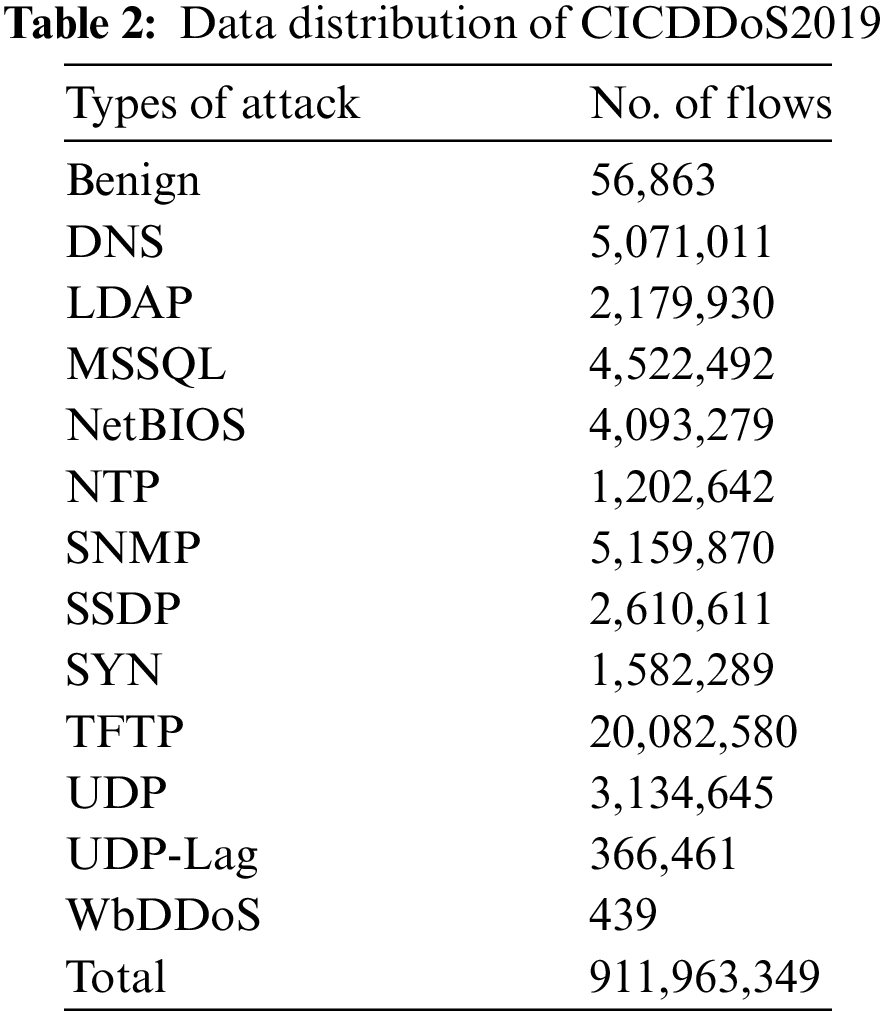
A new network intrusion dataset has been selected named CICDDoS2019, designed in 2019; the dataset consists of a large number of various types of DDoS attacks that can be carried out using Transmission Control Protocol (TCP) and User Datagram Protocol (UDP) at the application layer. The taxonomy of the DDoS attacks in the dataset is implemented in terms of reflection-based and exploitation-based attacks. The dataset is organized in two days for training and testing evaluation. The training set contains 12 different types, and the testing set contains 7 types of DDoS attacks. The dataset has more than 80 features, which were extracted using the CICFlowMeter tool. The distribution of the CICDDoS2019 data is described in Table 2.

5.1.2 LITNET-2020

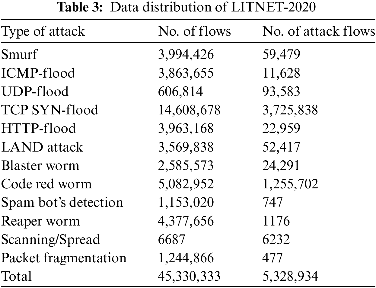
The LITNET-2020 NetFlow is a new dataset obtained from a real-world academic network. The network topology of the dataset consists of two parts: senders and collectors. The senders are Cisco routers and Fortige (FG-1500D) firewalls, which were utilized to process NetFlow data and send it to the collectors. The collector is a server with appropriate software that is responsible for receiving, storing, and filtering data. The LITNET-2020 dataset represented real-world examples of normal and attack traffic with 12 types of DDoS attacks. The total flow of the data samples is 45,492,310 flows, categorized into normal data with 45,330,333 flows and attack data with 5,328,934 flows. The LITNET-2020 dataset consists of 85 network features divided into 49 features that are specified to the NetFlow V9 protocol, 15 features are supplemented by the data extender, 19 features are offered to recognize attack types, and 2 additional features to determine the attack type and normal traffic. The distribution of attacks in the dataset. The distribution of LITNET-2020 data is described in Table 3.

5.2 Data Preprocessing

In data preprocessing, we divide the task into five steps, including features mapping, computing the missing value, feature selections, data normalization, and data imbalance.

5.2.1 Features Mapping

The data features in IoMT don’t contain only numeric values. So, a mapping technique is required to convert the categorical values to numeric values. One-Hot Encoding (OHE) technique converts the categorical features to integer format to be more expressive. The OHE transforms a single value with n features and d distinct values to d binary values with n features. Each feature indicates the presence of 1 or the absence of 0 of the dichotomous binary value. Using the OHE technique helps the deep learning models deal with the numeric values effectively.

5.2.2 Computing Missing Value

The datasets always consist of many missing values, which come from different reasons such as data failure or corruption during its recording, unreliable data transmission, and system maintenance and storage issues. The missing value is calculated using a linear interpolation method as

EF(xi)={∑k=i−5i+5PkUk×Averagelocalifxi∈NaNxiifxi∉NaN(30)

The Averagelocal computed as

Averagelocal=110×∑i−5i+5f(xi)(31)

where xi represents the data value, if xi is a null or non-numeric value, it is described as NaN. The Pk is the imputed data point between 0 and 1, and it is chosen to be 0.10 because the smallest value gives better performance. The Uk represents a binary value based on the threshold value of k. The threshold value is computed as

Uk={0ifxk<Averagelocal1ifxk≥Averagelocal(32)

5.2.3 Features Selection

Feature selection improves the quality of prediction during the selection of feature inputs. Feature selection is the process of converting the set of features into a subset that contains the features that are important to solve the detection problem and discard the unneeded features. In this paper, a Mutual Information (MI) technique is used for features selection. The criteria of selecting features are the dependency where the features that have high dependencies between them are noted as best features. The MI procedure is shown in the following steps:

Step 1: From the training set sample, the input-output variables can be represented as X and Y where S={X,Y}.

Step 2: The MI value between input and output variables MI(Xi,Y) measures the dependencies between them as

MI(X,Y)=∑x∈X∑y∈YP(x,y)logP(x,y)P(x)P(y)(33)

where P(x) and P(y) are the marginal distributions, and P(x,y) is the joint probability of X and Y.

Step 3: Remove the values which are less than other values and maintain the remaining values in vector M. The input-output variables represented as Snew. The Snew is sorting in descending order according to MI value from vector M.

Step 4: Define the number of selected features represented as f. Select the first f input-output variables from Snew as the selected feature to form set Sf.

Step 5: Select the variable with the highest MI value as the first variable in S. Select jth variables (1≤j≤f) from Sf and calculate the MI(S,Xj) values. The threshold is represented as α. If MI(S,Xj)≤α, S=S∪Xj. Otherwise, Xj will have less dependency and needs to be removed.

Step 6: Repeat Steps 4 and 5 until all variables are chosen.

5.2.4 Normalization

Normalization is a scaling method used to convert all features into a common scale. The minimum and maximum values range of the continuous feature in CICDDoS2019 and LITNET-2020 are different. A Min-Max is a popular method used to facilitate arithmetic processing, and the range of values of each feature is uniformly linearly mapped in the range between 0 and 1. The Min-Max scaling method can be defined as

Fscal=F−FminFmax−Fmin(34)

where Fscal represents the scaling data point, Fmin, and Fmax represent the minimum and maximum value of the input feature F.

5.2.5 Data Imbalance

The CICDDoS2019 and LITNET-2020s datasets are not perfectly balanced. The imbalanced dataset is solved using a Synthetic Minority Over-sampling Technique (SMOTE) [40]. SMOTE is an over-sampling technique used to avoid overfitting; it allows the generation of synthetic samples for the minority categories. It is based on the KNN algorithm, where it takes a sample from the dataset and considers its nearest neighbors in the feature map. If (x1,x2) is an example of a minority class and if its nearest neighbor is chosen as (x1´,x2´), then the data point is synthesized

(X1,X2)=(x1,x2)+random(0,1)×Δ(35)

where Δ={(x1´−x1),(x2´−x2)} and random (0,1) represent a random value in range [0, 1].

6  Experiments and Results

This section describes the experimental setup and the comparative analysis of the proposed DFSL system with baseline distributed algorithms such as FedAvg, Vanilla SL, and SplitFed with different experiments.

6.1 Experimental Setup

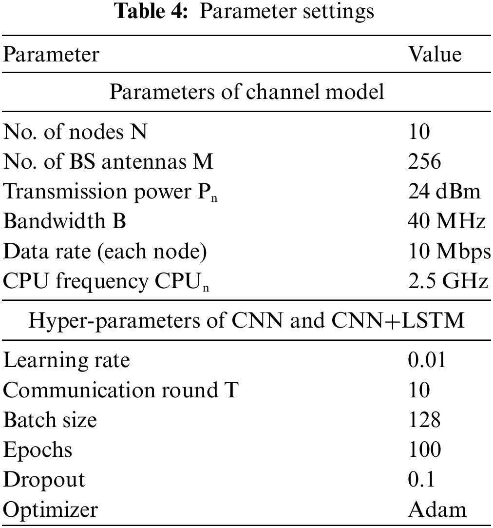
The experiment in this work is conducted with the following practical setting: Python version 3.7.3 and PyTorch library version 1.2 with Anaconda and CUDA version 10.1. We use a Dell laptop with CPU i5-1235U, 64-bit, GPU GTX 1050, and OS (Windows 11). The system consists of 10 fog nodes distributed at different distances from the server. We assume all fog nodes have the same computing capabilities. We use the 80:20 ratio (80% for the training set and 20% for the testing set). Using a high training set helps to ensure that the model is trained on enough datasets to capture the patterns and relationships in the data, and to learn more complex patterns. The tasks are assumed to be independent of each other. The parameter settings that are used in implementation are described in Table 4.

6.2 Performance Analysis

The proposed DFSL is compared with a baseline of distributed learning algorithms such as FedAvg, Vanilla SL, and SplitFed. The experiment is implemented with two datasets (CICDDoS2019 and LITNET-2020) on CNN and CNN+LSTM models to test the effectiveness of the proposed DFSL. The learning performance is implemented and compared based on four scenarios. First, the training loss and accuracy are tested with different cut layers. Second, the training time and communication overhead are tested with different numbers of nodes. Third, the adaptive aggregation of the DFSL will be compared with different aggregation methods. Finally, the proposed MNS scheme will be compared with different selection schemes.

6.2.1 Experiment 1: Performance Analysis of the DFSL with Different Cut Layers

The first experiment evaluates the proposed DFSL with different metrics such as loss, accuracy, and detection rate with different cut layers. Changing the cut layer point plays a huge role in the model’s effectiveness to get better results. We consider two types of model splitting represented by C={C1,C2}, where C2 means more layers assigned to the nodes. A smaller C should lead to a better performance because it corresponds to a larger part of the model server side, which better mitigates the non-IID issue. However, the results show that as C2 increases (i.e., more layers at the node side), the model performance increases. The impact of the cut layer becomes more significant, under which a larger C is more beneficial. To understand the reason behind this, we considered the evaluation with 10 nodes waiting for patience=10 rounds. We observe that the loss generally decreases, and accuracy and detection rate increase in C2, meaning a larger C leads to better model training. Also, the performance of CNN+LSTM is better than CNN, where adding LSTM layers positively affects the performance.

As shown in Fig. 8, the loss of DFSL outperforms FedAvg, Vanilla SL, and SplitFed with 0.07 and 0.02 at C2 in CICDDoS2019, and 0.05 and 0.01 in LITNET-2020 for CNN and CNN+LSTM, respectively. As shown in Fig. 9, the accuracy of DFSL outperforms FedAvg, Vanilla SL, and SplitFed with 98.99% and 99.70% at C2 in CICDDoS2019 and 99.50% and 99.87% in LITNET-2020 for CNN and CNN+LSTM, respectively. For detection rate, the DFSL outperforms the baseline algorithms with 98.14% and 99.60% at C2 in CICDDoS2019 and 98.89% and 99.60% in LITNET-2020 for CNN and CNN+LSTM, respectively. This improvement in loss and accuracy can be attributed to the adaptive aggregation method with predetermined the maximum loss and accuracy score.

Figure 8: Loss performance of CNN and CNN+LSTM (a) CICDDoS2019; (b) LITNET-2020

Figure 9: Accuracy performance of CNN and CNN+LSTM (a) CICDDoS2019; (b) LITNET-2020

In contrast, there is no big variation between FedAvg and SplitFed, as both apply the same aggregation strategy. For Vanilla SL, it scored the worst values in terms of loss, accuracy, and detection rate. It is very sensitive to data distribution. In fact, for both FedAvg and Vanilla SL, some knowledge forgetting while learning is evident when trained in non-IID settings.

When comparing the DFSL with the other approaches, we note that our DFSL has more hyper-parameters to tune when the cut layer is large. We conclude that a carefully specified way of determining the maximum accuracy and loss score and comparing it with average scores for each local update can benefit the most when applied in the DFSL system.

As shown in Tables 5 and 6, we observe that the proposed DFSL can detect DDoS attacks effectively enhancing learning performance. Based on these results, using the C2 version of our model has a better performance for detection.

6.2.2 Experiment 2: Performance Analysis of the DFSL with Different Number of Nodes

In this experiment, the training time and communication overhead are tested. We test the training time and communication overhead with different numbers of nodes, including N=10,30,and50 nodes. In Vanilla SL, only one node takes the whole bandwidth in each round because of its sequential training. In contrast, FedAvg, SplitFed, and DFSL are trained in parallel, so all selected nodes will share the whole bandwidth in each round. The performance was assessed on testing sets following the final communication round T. We observe that the increasing number of nodes increases the training time and communication overhead. In addition, the performance of CNN is better than CNN+LSTM because the model size negatively affects the training time and communication overhead, where a large model size needs to transmit more model parameters. So, the following results reflect the CNN result values.

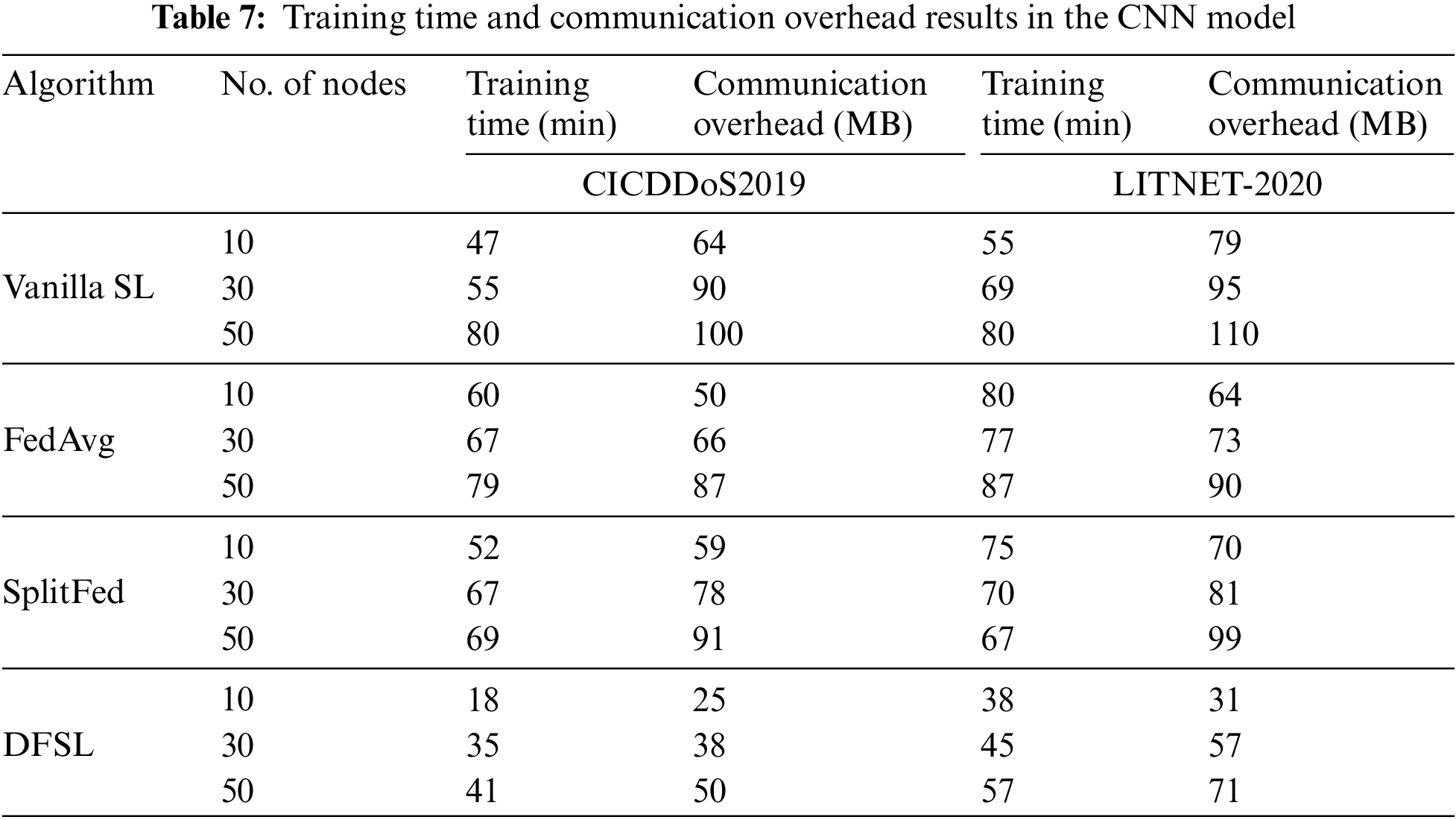
Fig. 10 shows the training time performance in CICDDoS2019 and LITNET-2020. The FedAvg has the highest training time compared with Vanilla SL, SplitFed, and DFSL, with 60 and 80 min in CICDDoS2019 and LITNET-2020, respectively, when the number of nodes is 10. The reason behind this is that in FedAvg, the allocated bandwidth to each node is decreasing. SplitFed achieves the highest training time after FedAvg with 60 and 80 min in CICDDoS2019 and LITNET-2020, respectively, when the number of nodes is 10. The Vanilla SL achieves acceptable results with 47 and 55 min in CICDDoS2019 and LITNET-2020, respectively. Compared to FedAvg, Vanilla SL, and SplitFed, DFSL spends less training time. The DFSL dynamically tunes the amount of computation assigned to the selected nodes at each round of training, resulting in a significant reduction in the overall training time per round. It achieves a total training time of 18 and 38 min in both datasets.

Figure 10: Training time performance (a) CICDDoS2019; (b) LITNET-2020

Fig. 11 shows the communication overhead in CICDDoS2019 and LITNET-2020. In terms of communication overhead, the performance degrades with increasing the number of nodes. When the nodes are 10, the DFSL has the lowest communication overhead with 25 and 31 MB in CICDDoS2019 and LITNET-2020, respectively. In contrast, FedAvg, Vanilla SL, and SplitFed with random node selection have high communication overhead. The Vanilla SL achieves 64 and 79 MB in CICDDoS2019 and LITNET-2020, respectively. The FedAvg has better performance than Vanilla SL, it achieved 50 and 64 MB in CICDDoS2019 and LITNET-2020, respectively. For SplitFed, it outperforms FedAvg and Vanilla SL with 59 and 70 MB. Finally, the DFSL with the proposed MNS scheme performs effectively on the performance. Selecting only the nodes with important update, good channel quality, and the nearest distance from the server reduces the communication overhead.

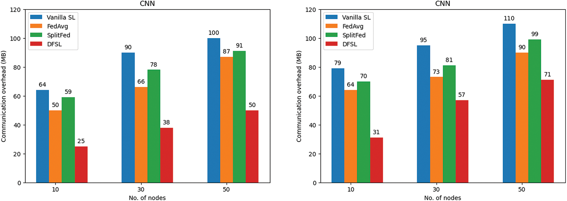
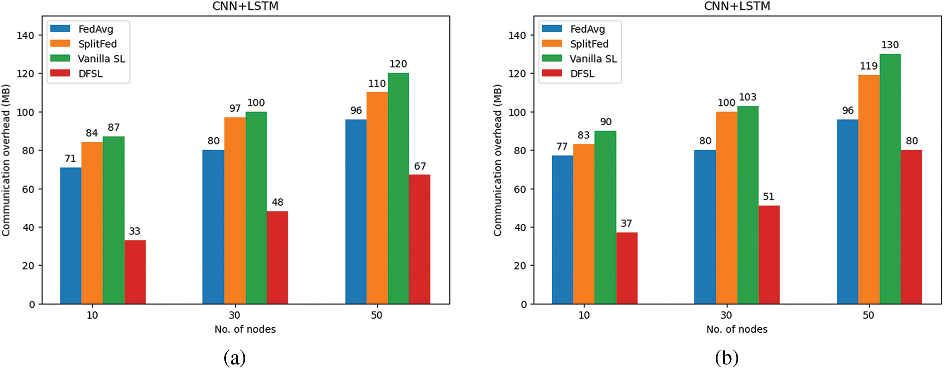
Figure 11: Communication overhead performance (a) CICDDoS2019; (b) LITNET-2020

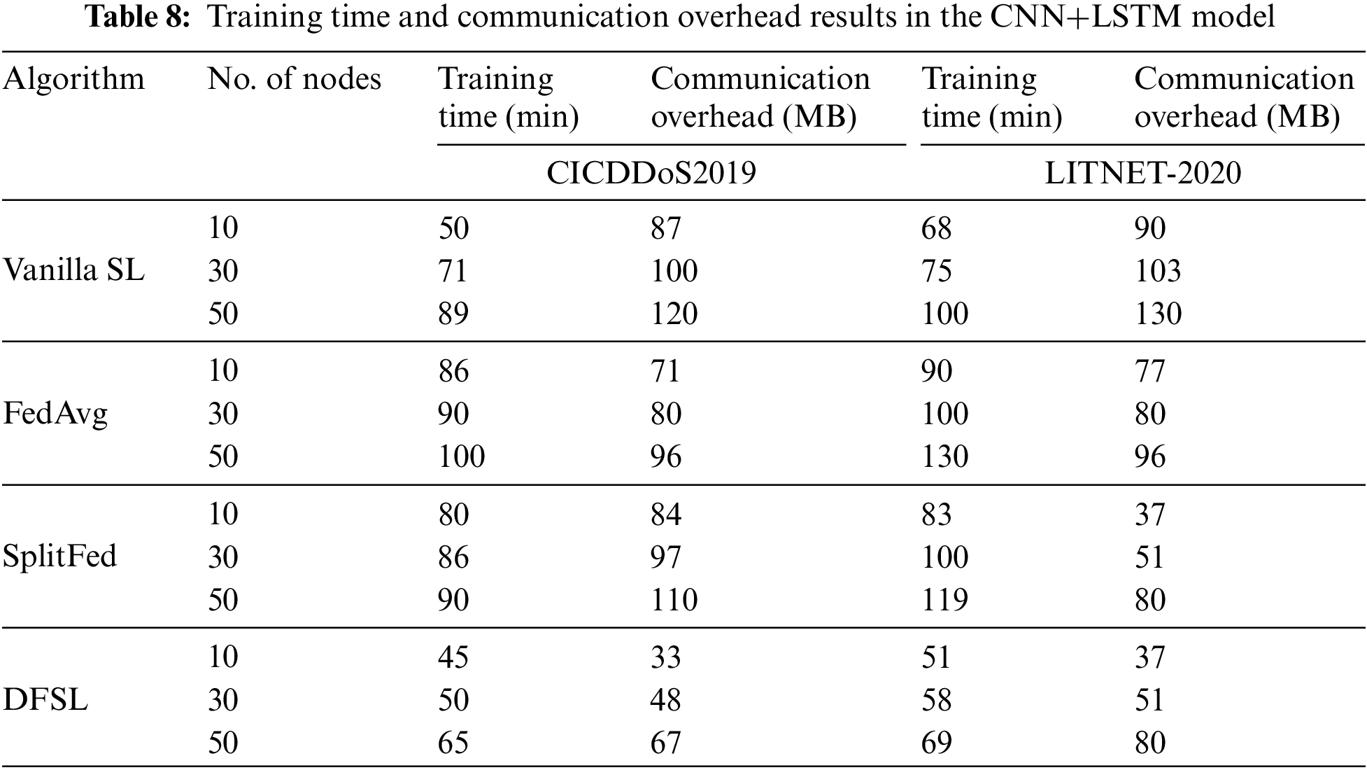
Tables 7 and 8 summarize the training time and communication overhead results with the increasing number of nodes for CNN and CNN+LSTM in CICDDoS2019 and LITNET-2020.

6.2.3 Comparing the Proposed Adaptive Aggregation with Other Aggregation Methods

The proposed adaptive aggregation in DFSL is compared with the three aggregation methods: geometric median [41], Krum aggregation function [42], and Fourier Transform [43], as shown in Table 9. We find that our aggregation method is more effective compared with the other methods. Determining the maximum score for accuracy and loss in each round enhances learning performance and makes the convergence more stable. Finally, we observe that our aggregation method gives more convergence stability without need for extra communications..

6.2.4 Comparing the Proposed MNS Scheme with Other Selection Schemes

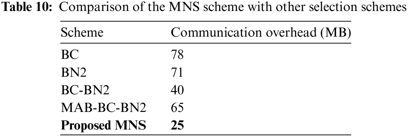
The proposed MNS scheme is compared with other selection schemes, such as BC, BN2, BS-BN2, and MAB-BC-BN2 schemes, as shown in Table 10. The MNS proves its effectiveness in reducing communication overhead compared with the other selection schemes. The dynamic selection of irrelevant updates and their exclusion during the training process helps to save computation and communication resources. Testing the performance of the MNS scheme by increasing the number of nodes proves that the MNS can be deployed in real-world IoMT with negligible additional computation overhead and thus can be implemented on a large scale.

6.2.5 Scalability Analysis

The above sections explain experiments in scenario with different nodes, including 10, 30, and 50 nodes, to test the training time and communication overhead. We assess DFSL’s performance across increasing DFSL sizes, measuring main metrics such as accuracy and convergence time (including ten rounds). To create the DFSL of extra sizes, we have increased the number of nodes up to 90 nodes.

The experiment has been executed 10 times for each DFSL size at each iteration. Fig. 12 shows the average accuracy and convergence time in LITNET-2020 dataset. The Figure shows that DFSL has consistent performance stability when the number of nodes increases. Furthermore, these results validate our proposed DFSL is stable with a large number of nodes.

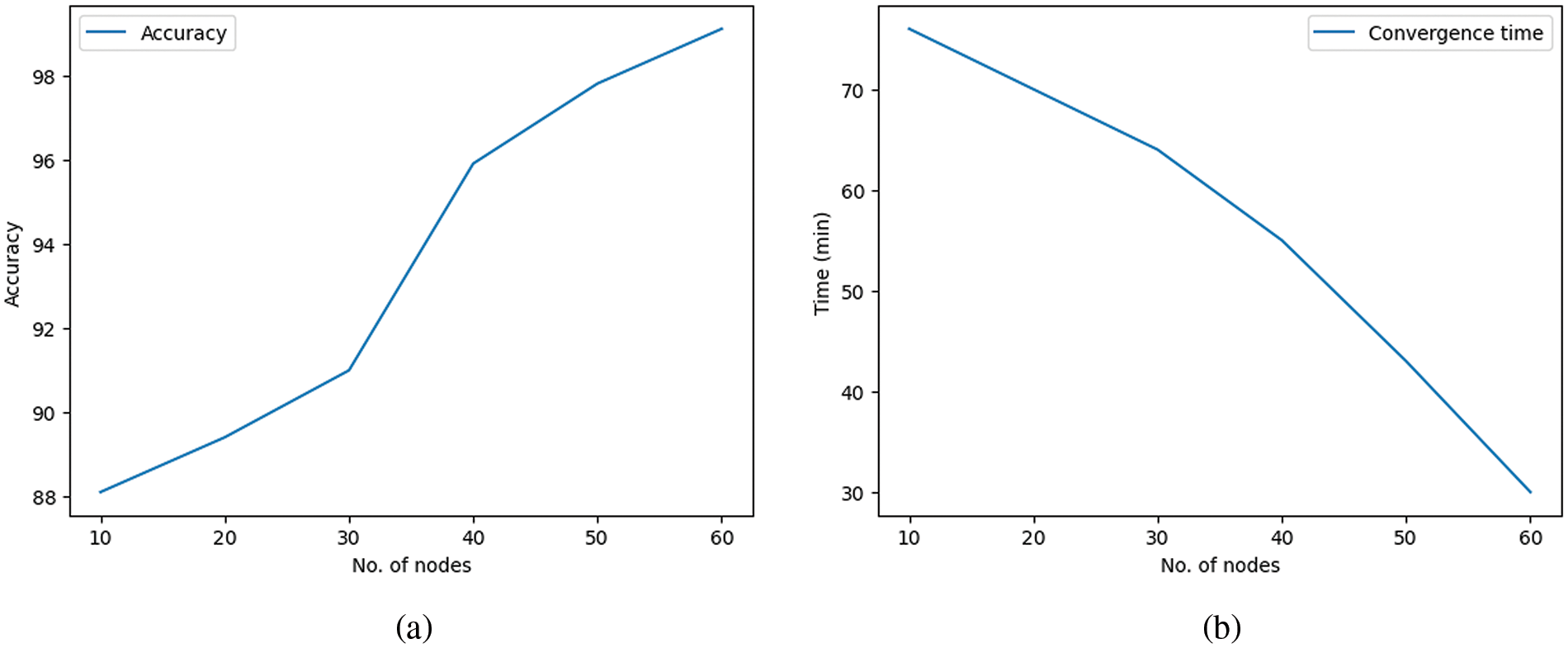
Figure 12: Scalability performance of the DFSL (a) accuracy; (b) convergence time

Therefore, with a few numbers of nodes, a low value on a few training sets can significantly impact on the overall average. In scenarios with more nodes, DFSL learns all attacks more accurately, although it consistently produces an accuracy below 0.93 when the number of nodes is 90.

The global model’s ability to perform well greatly impacts the DFSL process’s convergence time. By adding new nodes, the global model is learned more quickly, which has proven critical for the process’s convergence.

7  Discussion

In summary, the experiments’ results prove that the DFSL detects DDoS attacks with low loss value and high detection accuracy compared with the FedAvg, Vanilla SL, and SplitFed. In addition, it achieved low training time and communication overhead compared with FedAvg, Vanilla SL, and SplitFed.

In the first experiment, the DFSL training enhanced the model’s performance in terms of loss and accuracy when more layers were trained at the node side. We observe that the model’s performance achieves high accuracy and low loss by applying the early stopping strategy. In addition, we observe that the performance in LITNET-2020 is better than CICDDoS2019 performance; it contains more features and data to train. In the second experiment, stopping the model at a certain point when the model stops improvement helps to reduce training time. In contrast, the proposed MNS scheme helps to reduce communication overheads. It aims to decrease the communication rounds where only the important local update with good channel quality and the nearest node are selected for aggregation. It dynamically selects the relevant updates during the training process to avoid consuming computation and communication resources.

The model performance in CICDDoS2019 is better than LITNET-2020 in the second experiment, where more features need more training time and communication to transmit the model parameters.

Even though the proposed framework achieves acceptable results in terms of loss, accuracy, training time, and communication overhead, there are four implementation challenges and limitations of the proposed system, including:

1.   Achieving consistent accuracy: The data heterogeneity in IoMT across different nodes makes it a challenge to maintain constant accuracy results. Some nodes that have more heterogeneity rates need more training time for convergence.

2.   Anomalies data complexity: Notwithstanding our preprocessing efforts, some nodes sporadically presented anomalous data patterns. These could be attributed to distinct local network behaviors, which sometimes inject noise through model training.

3.   Real-time data: Although the proposed system is examined with two non-IID datasets proposed for DDoS attacks, it needs to be examined on real-time data to test its effectiveness.

4.   Real-time application: Although the proposed system is simulated by PyTorch, it needs to be examined in a real-time IoMT application.

8  Conclusion

A novel distributed FSL (DFSL) system is proposed in this paper to detect Distributed Denial of Service (DDoS) attacks in the IoMT networks while enhancing detection accuracy and reducing training time and communication overhead. The proposed system uses Federated Split Learning (FSL) to take advantage of each approach. The proposed system is tested on two DL models, including the Convolutional Neural Network (CNN) and a hybrid model that combines CNN and Long Short-Term Memory (LSTM) to determine the best model to detect DDoS attacks and test the effectiveness of the system. The procedure of the proposed system starts with initialization and model splitting, local model training, and adaptive aggregation. The adaptive aggregation method is designed based on the early stopping strategy to enhance learning performance and reduce training time. In addition, a Multi-Node Selection (MNS) based BC-BN2 selection scheme is proposed to reduce communication overhead with three selection metrics: the importance of local update, channel quality, and the nearest distance from the server. The performance results of the proposed system are compared with a baseline of distributed learning such as FedAvg, Vanilla SL, and SplitFed algorithms with different cut layers and increasing number of nodes. The results show the effectiveness of the proposed system where it can detect DDoS with an accuracy of 99.70% and 99.87%, and it achieved 18 and 38 min training time and 25 and 31 MB communication overhead in CICDDoS2019 and LITNET-2020, respectively. In future work, we aim to address the current limitations. We will further explore advanced convergence strategies with robust anomalous data management. In addition, we will deploy the proposed system in real IoMT scenarios to assess its feasibility in resource-constrained devices and networks.

Acknowledgement: The authors would like to extend their sincere thanks and gratitude to the supervisor for his support and direction of this research.

Funding Statement: The authors received no specific funding for this study.

Author Contributions: The authors confirm their contribution to the paper as follows: study conception and design: Rasha Almarshdi; data collection: Rasha Almarshdi; analysis and interpretation of results: Rasha Almarshdi, Etimad Fadel, Nahed Alowidi, Laila Nassef; draft manuscript preparation: Rasha Almarshdi, Etimad Fadel, Nahed Alowidi, Laila Nassef. All authors reviewed the results and approved the final version of the manuscript.

Availability of Data and Materials: The data supporting the contributions of this study are open-source and available at https://www.unb.ca/cic/datasets/ddos-2019.html and https://epubl.ktu.edu/object/elaba:61188126/ (accessed on 22 September 2024).

Ethics Approval: Not applicable.

Conflicts of Interest: The authors declare that they have no conflicts of interest to report regarding the present study.

References

1. S. A. Chelloug and M. A. El-Zawawy, “Middleware for Internet of Things: Survey and challenges,” Intell. Autom. Soft Comput., vol. 24, no. 2, pp. 309–318, 2018. doi: 10.1080/10798587.2017.1290328. [Google Scholar] [CrossRef]

2. D. Wang, D. Chen, B. Song, N. Guizani, X. Yu and X. Du, “From IoT to 5G I-IoT: The next generation IoT-based intelligent algorithms and 5G technologies,” IEEE Commun. Mag., vol. 56, no. 10, pp. 114–120, Oct. 2018. doi: 10.1109/MCOM.2018.1701310. [Google Scholar] [CrossRef]

3. S. Markkandan, S. Sivasubramanian, J. Mulerikkal, N. Shaik, B. Jackson and L. Naryanan, “Massive MIMO codebook design using gaussian mixture model based clustering,” Intell. Autom. Soft Comput., vol. 32, no. 1, pp. 361–375, 2022. doi: 10.32604/iasc.2022.021779. [Google Scholar] [CrossRef]

4. N. Javaid, A. Sher, H. Nasir, and N. Guizani, “Intelligence in IoT-based 5G networks: Opportunities and challenges,” IEEE Commun. Mag., vol. 56, no. 10, pp. 94–100, Oct. 2018. doi: 10.1109/MCOM.2018.1800036. [Google Scholar] [CrossRef]

5. M. Deepender, U. Shrivastava, and J. K. Verma, “A study on 5G technology and its applications in telecommunications,” IEEE Xplore, vol. 7, pp. 365–371, 2021. doi: 10.1109/ComPE53109.2021.9752402. [Google Scholar] [CrossRef]

6. A. Sonavane, A. Khamparia, and D. Gupta, “A systematic review on the internet of medical things: Techniques, open issues, and future directions,” Comput. Model. Eng. Sci., vol. 137, no. 2, pp. 1525–1550, 2023. doi: 10.32604/cmes.2023.028203. [Google Scholar] [CrossRef]

7. H. -C. Chen and S. -S. Kuo, “Active detecting DDoS attack approach based on entropy measurement for the next generation instant messaging app on smartphones,” Intell. Autom. Soft Comput., vol. 25, no. 1, pp. 217–228. doi: 10.31209/2018.100000057. [Google Scholar] [CrossRef]

8. S. Innes, “Banner Health paid $1.25 million to resolve Federal Data Breach Probe,” The Arizona Republic, 2023. Accessed: Feb. 03, 2023. [Online]. Available: https://www.azcentral.com/story/money/business/health/2023/02/04/banner-health-paid-1-25-million-to-resolve-federal-data-breach-probe/69871530007/. [Google Scholar]

9. Y. Ko, K. Choi, H. Jei, D. Lee, and S. Kim, “ALADDIN: Asymmetric centralized training for distributed deep learning,” in Proc. 30th ACM Int. Conf. Inform. Knowl. Manage., 2021, pp. 863–872. doi: 10.1145/3459637.3482412. [Google Scholar] [CrossRef]

10. S. Kamei and S. Taghipour, “A comparison study of centralized and decentralized federated learning approaches utilizing the transformer architecture for estimating remaining useful life,” Reliability Eng. Syst. Saf., vol. 233, May 2023, Art. no. 109130. doi: 10.1016/j.ress.2023.109130. [Google Scholar] [CrossRef]

11. N. N. Thilakarathne et al., “Federated learning for privacy-preserved medical internet of things,” Intell. Autom. Soft Comput., vol. 33, no. 1, pp. 157–172, 2022. doi: 10.32604/iasc.2022.023763. [Google Scholar] [CrossRef]

12. O. Gupta and R. Raskar, “Distributed learning of deep neural network over multiple agents,” J. Netw. Comput. Appl., vol. 116, pp. 1–8, Aug. 2018. doi: 10.1016/j.jnca.2018.05.003. [Google Scholar] [CrossRef]

13. Z. Zhang, A. Pinto, V. Turina, F. Esposito, and I. Matta, “Privacy and efficiency of communications in federated split learning,” IEEE Trans. Big Data, vol. 9, no. 5, pp. 1380–1391, Oct. 2023. doi: 10.1109/TBDATA.2023.3280405. [Google Scholar] [CrossRef]

14. M. M. Amiria, D. Gunduzb, S. R. Kulkarni, and H. V. Poor, “Convergence of update aware device scheduling for federated learning at the wireless edge,” IEEE Trans. Wirel. Commun., vol. 20, no. 6, pp. 3643–3658, 2021. doi: 10.1109/TWC.2021.3052681. [Google Scholar] [CrossRef]

15. X. Liu, Y. Deng, and T. Mahmoodi, “Wireless distributed learning: A new hybrid split and federated learning approach,” IEEE Trans. Wirel. Commun., vol. 22, no. 4, pp. 2650–2665, 2022. doi: 10.1109/twc.2022.3213411. [Google Scholar] [CrossRef]

16. T. Li, A. K. Sahu, A. Talwalkar, and V. Smith, “Federated learning: Challenges, methods, and future directions,” IEEE Signal Process. Mag., vol. 37, no. 3, pp. 50–60, May 2020. doi: 10.1109/MSP.2020.2975749. [Google Scholar] [CrossRef]

17. L. Collins, H. Hassani, A. Mokhtari, and S. Shakkottai, “FedAvg with fine tuning: Local updates lead to representation learning,” May 2022. doi: 10.48550/arxiv.2205.13692. [Google Scholar] [CrossRef]

18. J. Shen, X. Wang, N. Cheng, L. Ma, C. Zhou, and Y. Zhang, “Effectively heterogeneous federated learning: A pairing and split learning based approach,” in GLOBECOM 2023–2023 IEEE Glob. Commun. Conf., Kuala Lumpur, Malaysia, Dec. 2023, pp. 5847–5852. doi: 10.1109/GLOBECOM54140.2023.10437666. [Google Scholar] [CrossRef]

19. P. Vepakomma, O. Gupta, T. Swedish, and R. Raskar, “Split learning for health: Distributed deep learning without sharing raw patient data,” in Proc. Int. Conf. Learn. Rep. (ICLR) Workshop AI Social Good, 2019, pp. 1–7. doi: 10.48550/arXiv.1812.00564. [Google Scholar] [CrossRef]

20. C. Thapa, P. C. M. Arachchige, S. Camtepe, and L. Sun, “SplitFed: When federated learning meets split learning,” Proc. AAAI Conf. Artif. Intell., vol. 36, no. 8, pp. 8485–8493, Jun. 2022. doi: 10.1609/aaai.v36i8.20825. [Google Scholar] [CrossRef]

21. C. Huang, G. Tian, and M. Tang, “When minibatch SGB meets splitfed learning: Convergence analysis and performance evaluation,” 2023. doi: 10.48550/arXiv.2308.11953. [Google Scholar] [CrossRef]

22. Y. Mu and C. Shen, “Communication and storage efficient federated split learning,” in Proc. : ICC 2023-IEEE Int. Conf. Commun., May 2023, pp. 2976–2981. doi: 10.1109/icc45041.2023.10278891. [Google Scholar] [CrossRef]

23. A. Singh, P. Vepakomma, O. Gupta, and R. Raskar, “Detailed comparison of communication efficiency of split learning and federated learning,” 2019, arXiv:1909.09145. [Google Scholar]

24. Y. K. Saheed and M. O. Arowolo, “Efficient cyber attack detection on the internet of medical things-smart environment based on deep recurrent neural network and machine learning algorithms,” IEEE Access, vol. 9, pp. 161546–161554, 2021. doi: 10.1109/ACCESS.2021.3128837. [Google Scholar] [CrossRef]

25. M. Manimurugan, S. Al-Mutairi, M. M. Aborokbah, N. Chilamkurti, S. Ganesan and R. Patan, “Effective attack detection in internet of medical things smart environment using a deep belief neural network,” IEEE Access, vol. 8, pp. 77396–77404, 2020. doi: 10.1109/ACCESS.2020.2986013. [Google Scholar] [CrossRef]

26. M. Usman, M. A. Jan, X. He, and J. Chen, “P2DCA: A privacy-preserving-based data collection and analysis framework for IoMT applications,” IEEE J. Sel. Areas Commun., vol. 37, no. 6, pp. 1222–1230, Jun. 2019. doi: 10.1109/JSAC.2019.2904349. [Google Scholar] [CrossRef]

27. J. Ren, J. Guo, W. Qian, H. Yuan, X. Hao and J. Hu, “Building an effective intrusion detection system by using hybrid data optimization based on machine learning algorithms,” Secur. Commun. Netw., vol. 2019, pp. 1–11, Jun. 2019. doi: 10.1155/2019/7130868. [Google Scholar] [CrossRef]

28. S. P. K. Gudla, S. K. Bhoi, S. R. Nayak, and A. Verma, “DI-ADS: A deep intelligent distributed denial of service attack detection scheme for fog-based IoT applications,” Math. Probl. Eng., vol. 2022, pp. 1–17, Aug. 2022. doi: 10.1155/2022/3747302. [Google Scholar] [CrossRef]

29. R. Priyadarshini and R. K. Barik, “A deep learning based intelligent framework to mitigate DDoS attack in fog environment,” J. King Saud Univ.-Comput. Inf. Sci., vol. 34, no. 3, pp. 825–831, 2022. doi: 10.1016/j.jksuci.2019.04.010. [Google Scholar] [CrossRef]

30. Y. Zhang, Y. Liu, X. Guo, Z. Liu, X. Zhang and K. Liang, “A BiLSTM-based DDoS attack detection method for edge computing,” Energies, vol. 15, no. 21, Oct. 2022, Art. no. 7882. doi: 10.3390/en15217882. [Google Scholar] [CrossRef]

31. P. Verma, J. G. Breslin, and D. O’Shea, “FLDID: Federated learning enabled deep intrusion detection in smart manufacturing industries,” Sensors, vol. 22, no. 22, Nov. 2022, Art. no. 8974. doi: 10.3390/s22228974. [Google Scholar] [PubMed] [CrossRef]

32. V. Rey, P. M. Sánchez Sánchez, A. Huertas Celdrán, and G. Bovet, “Federated learning for malware detection in IoT devices,” Comput. Netw., vol. 204, Feb. 2022, Art. no. 108693. doi: 10.1016/j.comnet.2021.108693. [Google Scholar] [CrossRef]

33. Y. Alhasawi and S. Alghamdi, “Federated learning for decentralized DDoS attack detection in IoT networks,” IEEE Access, vol. 12, pp. 42357–42368, Jan. 2024. doi: 10.1109/ACCESS.2024.3378727. [Google Scholar] [CrossRef]

34. F. Yu, B. Zeng, K. Zhao, Z. Pang, and L. Wang, “Chronic poisoning: Backdoor attack against split learning,” Proc. AAAI Conf. Artif. Intell., vol. 38, no. 15, pp. 16531–16538, Mar. 2024. doi: 10.1609/aaai.v38i15.29591. [Google Scholar] [CrossRef]

35. S. Abuadbba et al., “Can we use split learning on 1D CNN models for privacy preserving training?,” in Proc. 15th ACM Asia Conf. Comput. Commun. Secur., 2020, pp. 305–318. doi: 10.1145/3320269.3384740. [Google Scholar] [CrossRef]

36. M. A. Khan, V. Shejwalkar, A. Houmansadr, and F. M. Anwar, “Security analysis of SplitFed learning,” in Proc. ACM Conf. Embed. Netw. Sens. Syst., Nov. 2022. doi: 10.1145/3560905.3568302. [Google Scholar] [CrossRef]

37. F. Li, J. Lin, and H. Han, “FSL: Federated sequential learning-based cyberattack detection for industrial Internet of Things,” Ind. Artif. Intell., vol. 1, Mar. 2023, Art. no. 4. doi: 10.1007/s44244-023-00006-2. [Google Scholar] [CrossRef]

38. I. Sharafaldin, A. H. Lashkari, S. Hakak, and A. A. Ghorbani, “Developing realistic distributed denial of service (DDoS) attack dataset and taxonomy,” in Proc. 2019 Int. Carnahan Conf. Secur. Technol. (ICCST), IEEE, Oct. 2019, pp. 1–8. doi: 10.1109/CCST.2019.8888419. [Google Scholar] [CrossRef]

39. R. Damasevicius et al., “LITNET-2020: An annotated real-world network flow dataset for network intrusion detection,” Electronics, vol. 9, no. 5, May 2020, Art. no. 800. doi: 10.3390/electronics9050800. [Google Scholar] [CrossRef]

40. A. Fernandez, S. Garcia, F. Herrera, and N. V. Chawla, “SMOTE for learning from imbalanced data: Progress and challenges, marking the 15-year anniversary,” J. Artif. Intell. Res., vol. 61, pp. 863–905, Apr. 2018. doi: 10.1613/jair.1.11192. [Google Scholar] [CrossRef]

41. K. Pillutla, S. M. Kakade, and Z. Harchaoui, “Robust aggregation for federated learning,” IEEE Trans. Signal Process., vol. 70, pp. 1142–1154, 2022. doi: 10.1109/TSP.2022.3153135. [Google Scholar] [CrossRef]

42. R. Taheri et al., “Robust aggregation function in federated learning,” in Proc. 6th Int. Conf. Inform. Knowl. Syst., Cham, Springer Nature Switzerland, 2023, pp. 168–175. doi: 10.1007/978-3-031-51664-1_12. [Google Scholar] [CrossRef]

43. E. M. Campos, A. Jose, L. Ramos, and A. Skarmeta, “FedRDF: A robust and dynamic aggregation function against poisoning attacks in federated learning,” 2024. doi: 10.48550/arXiv.2402.10082. [Google Scholar] [CrossRef]