Predicting Grain Orientations of 316 Stainless Steel Using Convolutional Neural Networks

1  Introduction

Steel is a critical material in various industries, and its production has advanced significantly. However, surface defects can occur due to raw material quality and production conditions, negatively impacting steel’s performance and durability. To ensure steel quality, inspecting for these defects during production is essential, as they can have profound consequences [1].

In recent years, convolutional neural networks (CNNs) have become increasingly popular for image analysis and classification tasks. In materials informatics, deep learning analyzes image data and predicts material properties. Deep learning algorithms are trained on large datasets of images and associated material properties. The algorithms then learn to recognize patterns in the data that can be used to predict the material properties of unseen images accurately. This approach has been successfully applied to various materials, including metals, polymers, ceramics, and composites. Deep learning has also been used to develop new materials with desired characteristics. By training deep learning models on existing material datasets, researchers can identify patterns in the data that can be used to generate new materials with desired properties. This approach has been used to develop and predict new alloys with improved strength and corrosion resistance and new polymers with enhanced thermal stability and mechanical strength.

Materials science and engineering scientists use experiments and simulations to identify the processing structure property performance (PSPP) relationships, such as multiscale complexity, limited data availability, and computational power requirements, even though these connections are not yet fully understood. Understanding the PSPP allows for the design, optimization, and tailoring of materials to meet specific requirements, improve performance, and control manufacturing processes. Indeed, all aspects of materials science hinge on these PSPP connections. It is essential to grasp this intricate system better to discover and create new materials with the desirable attributes [2].

Deep learning has become an asset in analyzing large datasets; it implements intricate algorithms and AI neural networks to enable machines to comprehend, classify, and define images like the human brain does [3]. CNN is an AI neural network commonly utilized in deep learning to identify and label visual elements. Using CNN, deep learning can detect objects within images [4].

CNNs are significant for multiple purposes, including image analysis and machine vision processes like determining position together with division. They can also be used with microscopy technologies to anticipate fractures in materials by detecting grains and edges. In addition, CNNs are highly sought-after in deep learning since they are essential in the current and emerging arenas [5].

Furthermore, Electron Backscatter Diffraction (EBSD) is a method employed to study the orientation of materials in terms of crystallography. It is used to examine the structure of materials at the atomic level. A beam of electrons with great energy is projected onto the sample being studied, and the electrons that hit the surface are reflected in different directions due to the depths and lattice orientations. The pattern of the reflected electrons is identified by a phosphor screen detector, which typically has bright parallel and intersecting greyscale bands. When the specimen is tilted or shifted, the bands’ arrangement alters since the crystal lattice’s orientation shifts. This technique primarily focuses on crystal orientation. The most common technique used for indexing EBSD is based on the Hough transform. This technique relies on calculating the angles formed by linear features derived from the directional configuration. A significant challenge posed by this approach is its high sensitivity to noise, which significantly decreases its accuracy [2].

This article investigates the feasibility of utilizing a deep learning neural network to create a model that can predict the orientation of grains exposed to various deformation factors, such as temperature and strain rate. The current work demonstrates a groundbreaking methodology since it can anticipate the crystallography of substances, obviating the need for time-consuming EBSD analysis. The paper also reveals how the pattern shifts from deformation, allowing the process to be altered to obtain the preferred grain orientations. This paper is divided into seven sections: Section 2 discusses EBSD methodology, Section 3 provides information on the experiments, Section 4 covers machine learning concepts and techniques, Section 5 describes the deep learning algorithm and the trained models, Section 6 evaluates the model and results, and Section 7 concludes the paper.

2  Electron Backscatter Diffraction (EBSD)

Numerous deep learning networks have been employed to analyze and process material images. One of the common techniques for training deep learning models in material science is the use of EBSD. A scanning electron microscope (SEM) is employed to analyze the microscopic structure of a sample. When the electron beam interacts with the tilted crystal-line sample, the scattered electrons generate a pattern that can be seen on a fluorescent screen. The diffraction pattern generated by the electron beam reveals the crystal structure and orientation of the sample. This information can determine the sample’s crystal orientation, different phases, grain boundaries, and local crystalline perfection. Over the past few years, EBSD has become a popular complement to the SEM, offering quick insight into the crystallographic features of a sample. Consequently, EBSD is being utilized in various applications to support the characterization of materials [6–7].

EBSD has become a widely accepted tool, along with the scanning electron microscope. This technique provides details about the crystal structure and is used in various projects to support material analysis [8].

Liu et al. [9] developed an early deep learning approach for EBSD indexing. The aim is to offer a comprehensive approach that eliminates the need for specialized knowledge or visual data processing technology. The method relies on the insertion of the raw EBSD images so that the three numerical values can be predicted using CNNs designed to recognize the structural relationships among the pixels and extract the applicable characteristics. The system comprises multiple levels, including pooling to lower the number of parameters and connected layers for the predicted regression.

Historically, material research focused on altering the composition and processing of material to achieve the desired microstructure and performance. However, this technique was characterized by a high degree of manual effort and reliance on trial and error. This led to the proposal of the Material Genome Project in several countries to speed up the research and development of new materials. This project aims to establish a link between the composition and process, organizational structure, and material performance. As such, the main goal is to create a quantitative relation between the composition/process and the performance of the material [10].

Shu et al. [11] researched material characteristics prediction using EBSD, one of the most precise ways to characterize material. This characterization data contains structural details, and computers can easily interpret them. Consequently, they developed an EBSD-based digital knowledge graph representation, followed by the design of a representation learning system to incorporate graph characteristics. They could predict material behavior by inputting the graph into an artificial neural network. They conducted experiments on magnesium metal to assess their approach and compared the results to those from established machine learning and computer vision approaches. Their discoveries showed the precision of their proposed method and its value for calculating properties. They created a way of illustrating the EBSD grain data graph, which can be employed to predict organizational performance.

They utilized vertex and connection representations to create a convolutional network for graph features, which incorporated the graph-based knowledge and enabled the retrieval of network features. Subsequently, a feature map-ping network based on a neural network was formulated with the graph feature to forecast material properties.

The researchers created a Convolution Network for Graph Features that aims to utilize the grain-based knowledge database and extract network features. Subsequently, a Neural Network-based Feature Mapping Network was constructed to forecast material characteristics. They compared their method to two other strategies: conventional statistics machine learning and visual element extraction based on computer vision. To assess material properties, conventional machine learning techniques were employed to compute the attribute characteristics of all grains, such as Ridges, support vector regression (SVR), k-nearest neighbors (KNN), and Decision Trees. These are common machine learning algorithms. Additionally, the CNN model was utilized to extract visual components from the microstructure guide and anticipate execution. The CNN technique has been consistently proven to be the most effective and reliable solution compared to other methods. Its indisputable superiority makes it the preferred choice for many [11].

3  Experimental Work

We initiated our investigation by machining the 316 stainless steel alloy. The sample was cut into a cylindrical shape of 5 mm in diameter and 10 mm in length. The rods were subjected to a heat treatment of 1050°C for 1 h for homogenization. The rod-shaped configuration is visualized in Fig. 1a. To ensure uniformity, some areas of the material were explored for the microstructure, both pre and post-treatment, as seen in Fig. 1b. Figs. 2 to 4 illustrate the microstructure at various levels, demonstrating the grains’ uniformity and arrangement. Table 1 outlines the chemical composition of stainless-steel alloy 316.

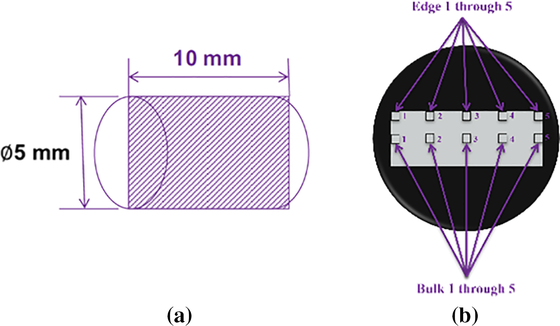
Figure 1: Details of the specimen: (a) Dimensions of the sample; (b) Locations of the sample

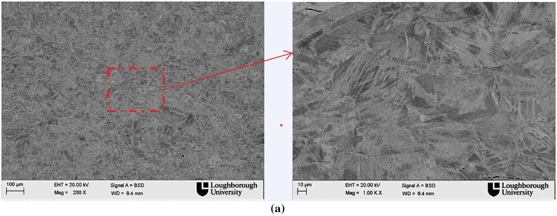
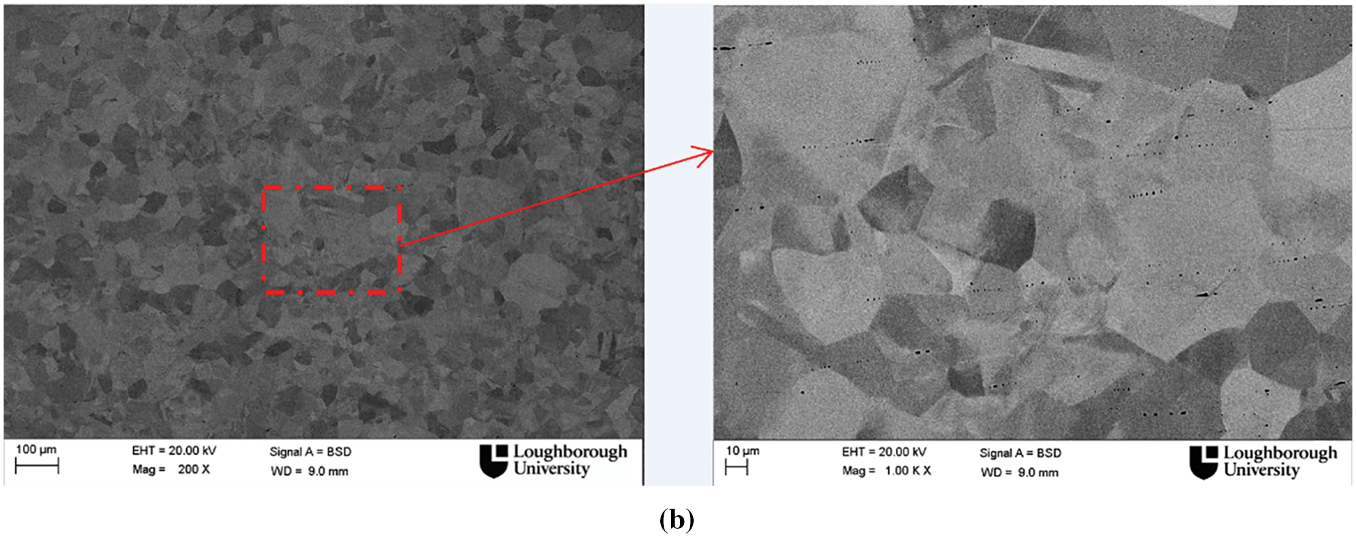
Figure 2: SS316 homogenization process: (a) Original state; (b) After processing

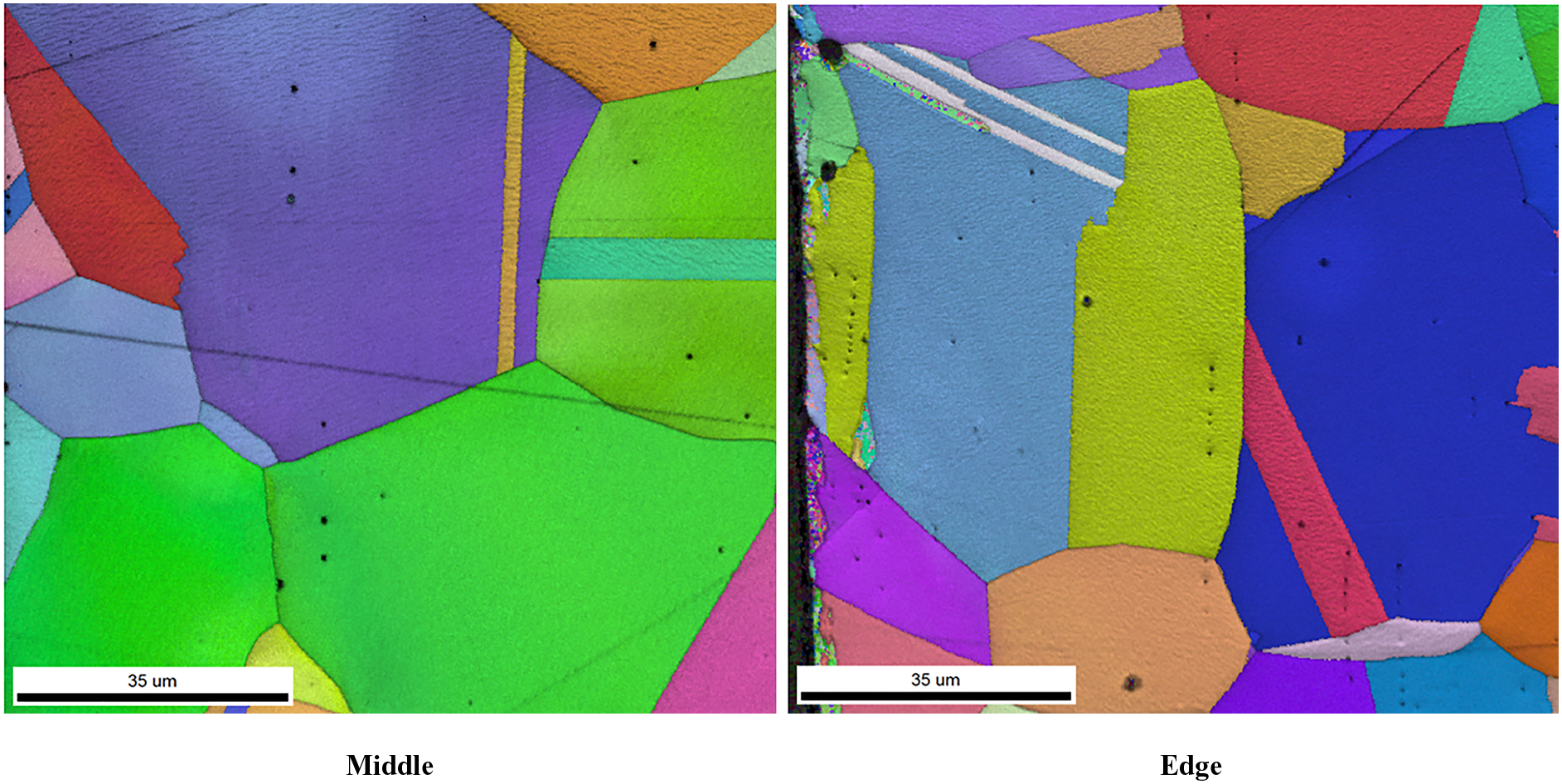
Figure 3: SS316 homogenization

Figure 4: SS316 EBSD of the homogenized material

Table 2 exhibits the results of annealing treatment deformation when conducted at various temperatures and strain rates. Theoretically, every sample should have a final length of 9.8 mm (starting from 10 mm). To obtain an EBSD map, all SS316 alloy samples were prepared, and their initial and post-deformation sizes were measured and documented.

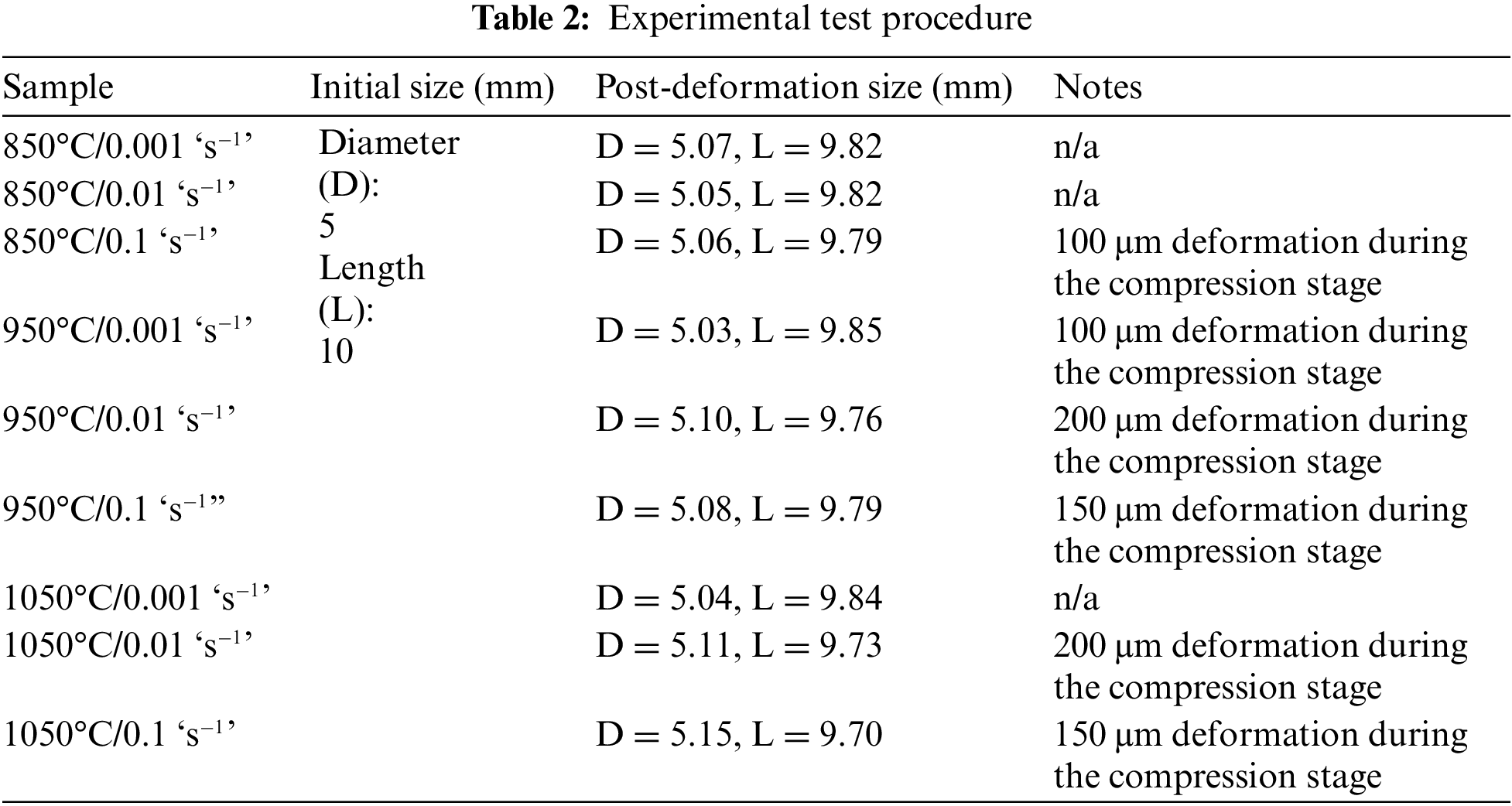
To measure the effect of strain and temperature on the kinetics of static recrystallization, specimens were exposed to pressure, then water-quenched, and cut into eight sections to generate a recrystallization curve. After mechanical polishing, the samples were electro-etched in a 10% solution of oxalic acid solution. The presence of recrystallized grains was evident due to their reduced size and stress-free microstructure. The material’s behavior indicates that strain hardening occurs throughout the stress application. However, the amount of strain hardening for the observed increment in the stress decreases as stress increases. Fig. 5 illustrates the outcomes of deforming SS316 alloy samples under various strain rates and temperatures. Theoretically, every sample should have a final length of 9.8 mm (starting from 10 mm). To get an EBSD map, all SS316 alloy samples were prepared, and their initial and post-deformation sizes were measured and recorded [12].

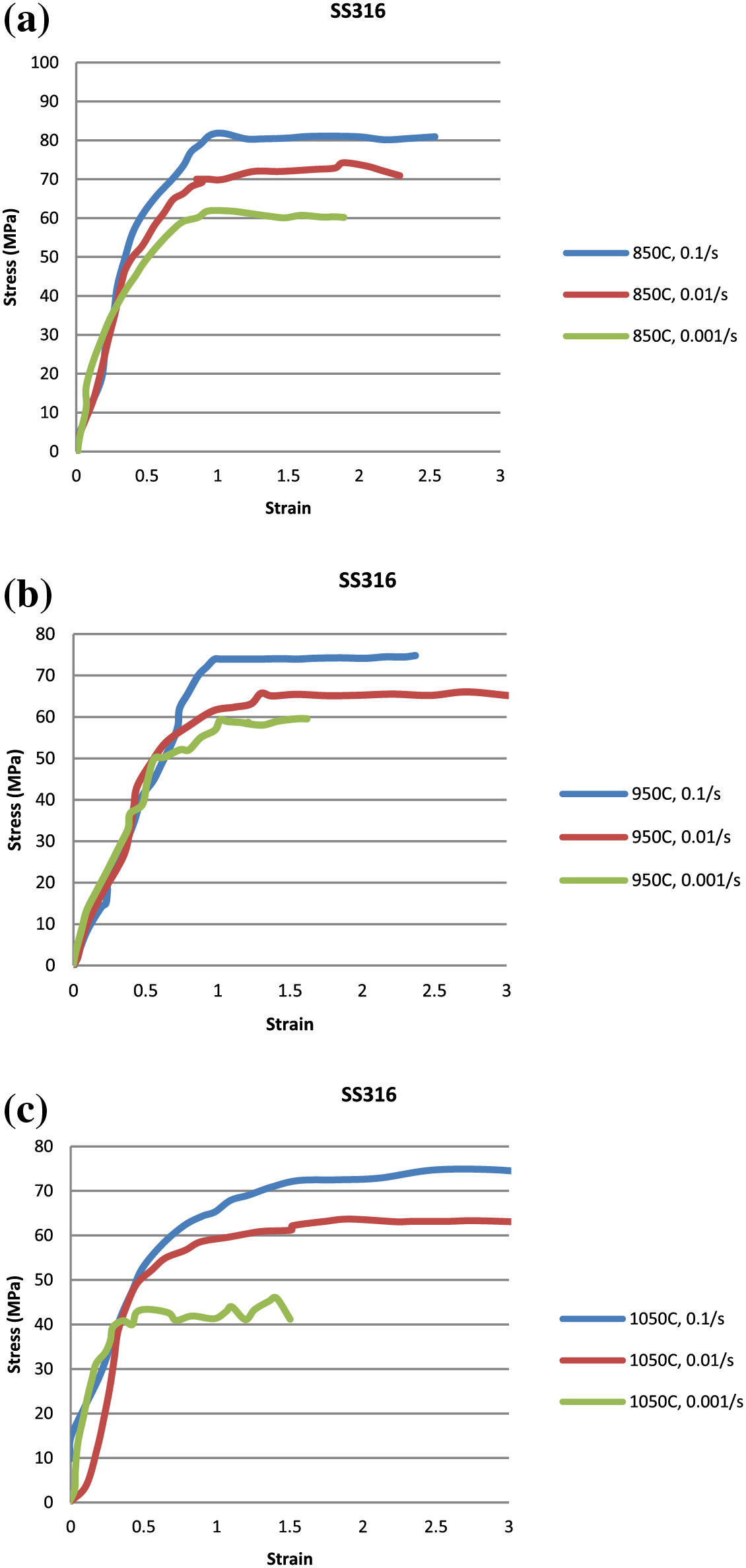
Figure 5: Schemes SS316 strain/stress results: (a) 850°C; (b) 950°C; (c) 1050°C

Figs. 6–14 show the misshapen recrystallized items according to the various deformations, polishing, and electron backscatter diffraction.

Figure 6: 850°C, 0.001/s

Figure 7: 850°C, 0.01/s

Figure 8: 850°C, 0.1/s

Figure 9: 950°C, 0.001/s

Figure 10: 950°C, 0.01/s

Figure 11: 950°C, 0.1/s

Figure 12: 1050°C, 0.001/s

Figure 13: 1050°C, 0.01/s

Figure 14: 1050°C, 0.1/s

4  Machine Learning

Deep learning, a subfield of machine learning, employs multi-layered neural networks with three or more layers. These networks process large amounts of data, mimicking the human brain to improve accuracy. While a single-layer network might make rough predictions, multiple layers enhance precision [13].

Many AI applications now use deep learning to automate tasks without human involvement [14]. Agrawal et al. [2] noted that deep learning marks a resurgence of neural networks from the 1980s. With more data and computing power, these networks have become more complex, impacting fields like computer vision and speech recognition.

Goodfellow et al. [15] refer to the multilayer perceptron (MLP) as the conventional deep learning architecture. An MLP can be viewed as a computational equation generating precise outputs from inputs. Each layer represents a state of computer memory after executing instructions, allowing deeper networks to handle multiple tasks simultaneously [16].

In summary, deep learning enables computers to become smarter through data and experience. Various models, including CNNs, have been used to solve problems beyond human comprehension.

4.1 Convolutional Neural Networks

CNN is an artificial neural network that processes and identifies patterns in large datasets by automatically learning and extracting features, thereby capturing complex patterns and relationships. CNNs are composed of multiple layers and weights, which are trained to identify patterns in the data. The trained model is then used to make predictions on new data. By leveraging CNN’s capabilities, several tasks, such as image recognition, natural language processing (NLP), speech recognition, and data mining, can be executed quickly and accurately [17].

Time-series information is a sequence of samples taken at consistent intervals, while image data is a two-dimensional array of pixels. Convolutional networks have experienced excellent results in practical applications, which is part of linear algebra. CNNs, also known as Convolutional Neural Networks, include at least one layer that employs convolution rather than conventional matrix multiplication. This has enabled them to be used in various fields, from image recognition to speech recognition and beyond [16].

4.2 Structure of CNN

CNN has three primary components: a convolutional layer, a pooling layer, and a fully connected layer.

4.2.1 The Convolutional Layer

The basis of a convolutional neural network consists of a range of layers that generate its parameters. Despite being small, these layers process the input data to detect more significant features and generate the network’s parameters. The initial layer recognizes low-level features, such as color, edges, etc. Subsequent convolutional layers filter out the high-level features, providing a comprehensive image understanding.

4.2.2 The Pooling Layer

This layer aims to shrink the visual representation, resulting in fewer computations and fewer processing needs for the neural network. This then draws out dominant features that remain unchanged regardless of the position or orientation.

Max pooling is a technique that considers the most essential value from every neuron cluster of the layer before it. This is compared to Average pooling, which produces the average of a neuron cluster. Max pooling has the advantage of being a noise suppressor, making it preferable over Average pooling. Convolutional layers are not the only type used in feature extraction from an image. Including more pooling layers can create poor features, requiring increased computational power. After the convolutional and pooling layers have been processed, the feature extraction process is finished.

4.2.3 The Fully Connected Layers

The concluding step is the fully connected layer, otherwise known as a feed-forward neural network. This layer takes a 3-dimensional matrix/array and generates a vector passed on from the preceding pooling layer as input.

Every fully connected layer carries out a distinct mathematical operation. After all the FC layers have processed the vector, the SoftMax activation function is employed in the final layer, which facilitates the neuron’s output to determine the probability that the input is related to a specific task. As a result, the final output consists of the probability that the input image pertains to diverse classes. The exact process is done with multiple image types and the images within each type to train the network to differentiate between different images [18].

Deep learning convolutional neural networks are emerging as powerful and effective techniques for developing and analyzing materials. The expansion of repositories supplying images and raw data to researchers has created an opportunity for data science to revolutionize the process of materials prediction. New algorithms and tools reveal the potential for successful material prediction outcomes and the advancement of cutting-edge materials.

Using deep learning, convolution neural network techniques is a superior way to progress material development and analysis. Data-driven approaches, utilized with immense success over a wide range of material data, are increasingly adopted in computer science. Researchers can gain access to an array of data repositories containing images and raw data, enabling them to conduct in-depth analysis. Meanwhile, the ongoing progress in data science has produced novel algorithms to investigate data. This could be very beneficial in meeting the materials prediction goals and helping to find, devise, and implement the newest materials [19–20].

5  Deep Learning

5.1 CNN Training

An Artificial Intelligence (AI) system has been used to generate EBSD images that are 1279 × 375. Both size and length both change in the same direction as it rolls (Fig. 3). Due to the multiple deformation conditions, more than two thousand grains were taken from each EBSD. A total of around 20,000-grain orientations are utilized in the training and testing process. An AI algorithm is trained using grain orientations as input.

Rather than reducing the image’s resolution by descaling it, the image was split into smaller sections to reduce the total amount of source images. This was necessary due to a lack of space. After eliminating the low-luminance edges and the drawing scale, each EBSD image was split into eight images of 450 × 150 dimensions. CNNs are very sensitive to changes in images in terms of color, brightness, and additional objects unrelated to orientation, such as text and symbols. Hence, the images must be normalized to obtain superior results.

Both a classifier and a predictor were employed during the implementation of the deep learning algorithm. The classifier was used to identify the circumstances in which the material was deformed, and the predictor was utilized to compute how the grain orientations would be altered due to the deformation. The first network, based on CNN, was educated with MATLAB’s deep learning algorithm, and the second network, based on a Long-Short-Term-Memory Neural Network (LSTM) and predicted grain orientation, was trained with LSTM. On the output side of the supervised learning, sigmoid functions were used, while ReLU activation functions were employed on the input side of the unsupervised learning. MATLAB was used to implement the algorithms, and an i5 machine was used to run them. Multiple processes were conducted to acquire the most suitable model, and the result of the most successful run was then compared to the results of the other runs to find out which one produced the most precise network. Fig. 15 illustrates this.

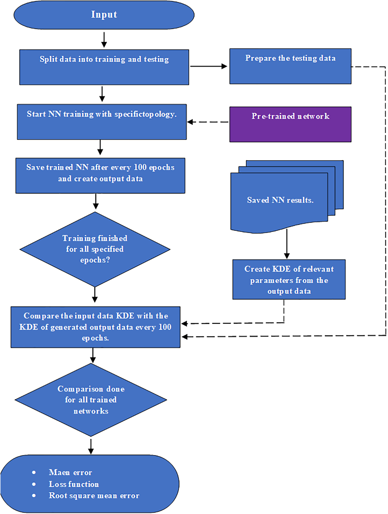
Figure 15: CNN training, validation errors, and loss function flowchart

CNN utilizes three color channels—red, green, and blue—as inputs, known as RGB. Once the input is put through multi-color convolution, the output is broken down into ten sections, showing the particles’ orientation as shown in Fig. 16. The framework comprises three stages, the first of which involves an 8-filter stage, then a 16-filter stage, and the last is a 32-filter stage. The size of each filter is three by three. The last stage is a fully connected layer with ten classes that show each deformation state. To prepare the system for identifying grains misaligned because of deformation, non-deformed images are utilized to train the algorithms and configure the network. The data is divided into two parts, the training and the testing data, which are then subjected to the contrastive divergence search algorithm. This algorithm assesses the cost function by processing the data in small batches, and as a result, the network weights are adjusted. Repeating the training batches one after the other is named an epoch, with a batch size of ten used for the entire training [15].

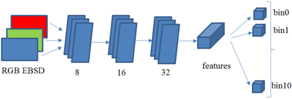
Figure 16: CNN topology

This experiment employed Root-Mean-Square Error (RMSE) to measure the value of the prediction. Data was divided randomly, with 80% for training and 20% for testing. The training process was monitored every 10 epochs to avoid overfitting. The training phase had a total of five hundred epochs. After the training procedure was completed, the optimal fit was chosen and tested. Fig. 17 illustrates the training and validation processes, along with the error and loss functions for both datasets. RMSE observed during the validation procedure was 14.79.

Figure 17: CNN training, validation errors, and loss function

5.2 Grain Orientation Modelling

The EBSD images show the grain orientation as color-coded. Hence, RGB represents the grain orientation. The spatial and angular distribution is considered to predict the orientation of the grains. A color triangle is shown in Fig. 18 to show the orientation of grains with the help of colors. Red grains are associated with 001, green with 111, and blue with 101 [21]. Orientation can be determined by looking at the RGB color map. This map comprises a range of 256 numbers, with zero being black and 256 being white. Red is assigned a number of 76; blue is given 30, and green is 150. Therefore, 001 grains would indicate seventy-six marks, 111 grains would indicate 150, and 101 grains would be at 30. Fig. 19 displays a histogram of the grain distribution from each EBSD map and grain modeling in Fig. 20. The strain rates deformation at three different temperatures (850°C, 950°C, and 1050°C) [22]. The orientation of the grain is based on the EBSD image. Since CNN works with images, the color of the grain is an indication of the orientation. Hence, CNN learned the orientation based on the color of the EBSD image.

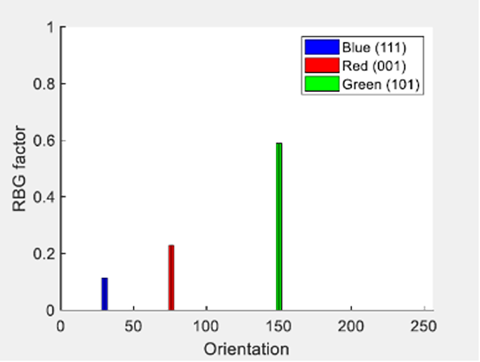
Figure 18: Grain orientation color map

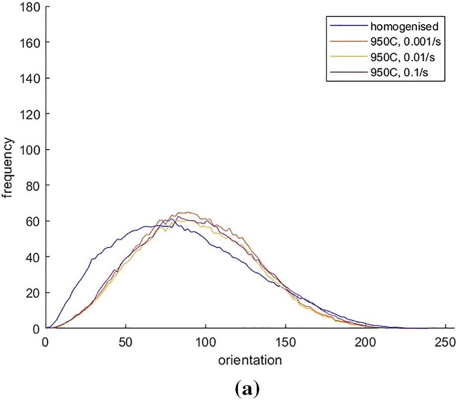
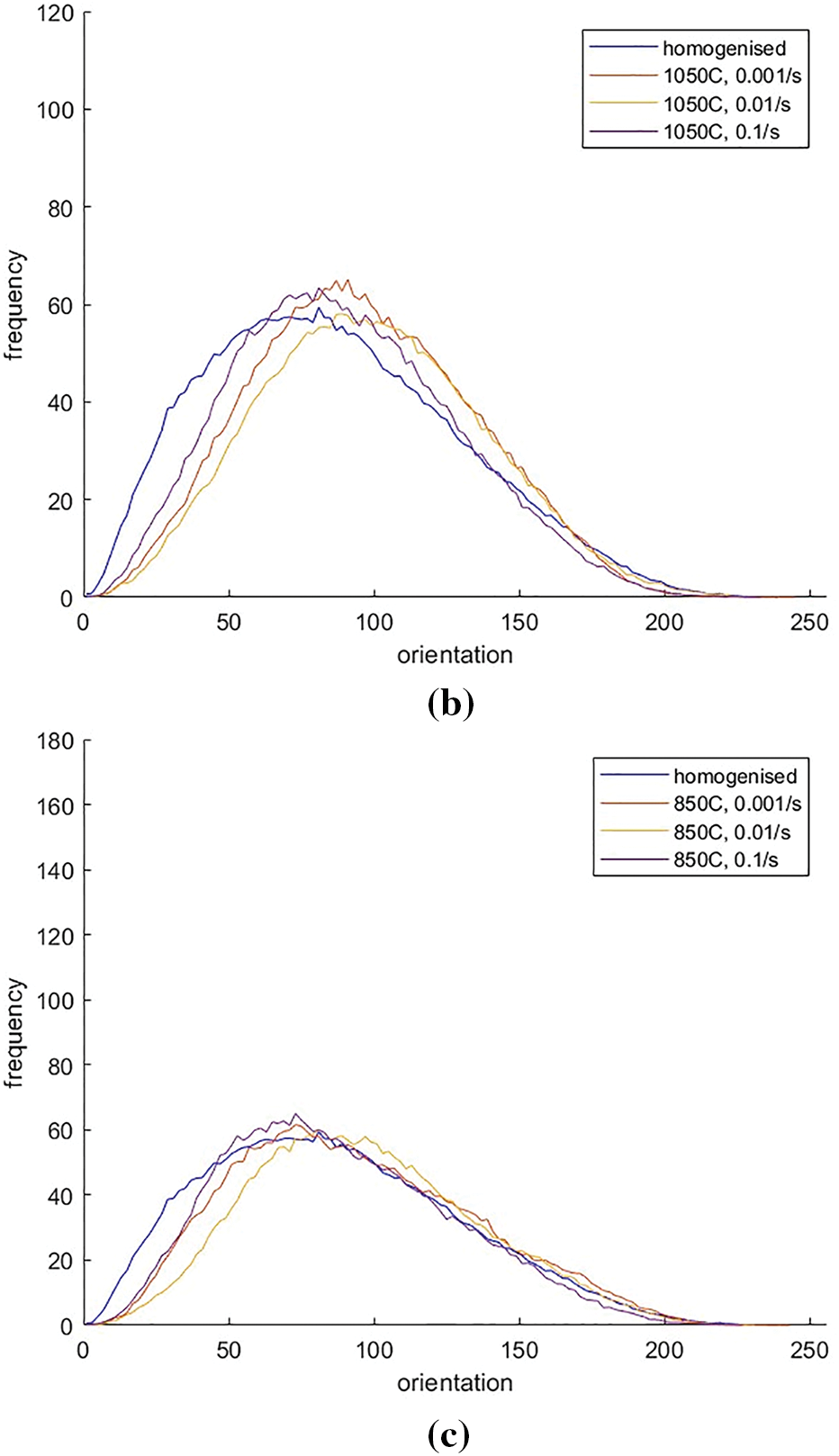
Figure 19: EBSD grain orientation histogram of the deformed materials

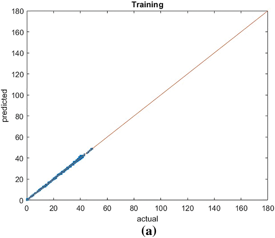
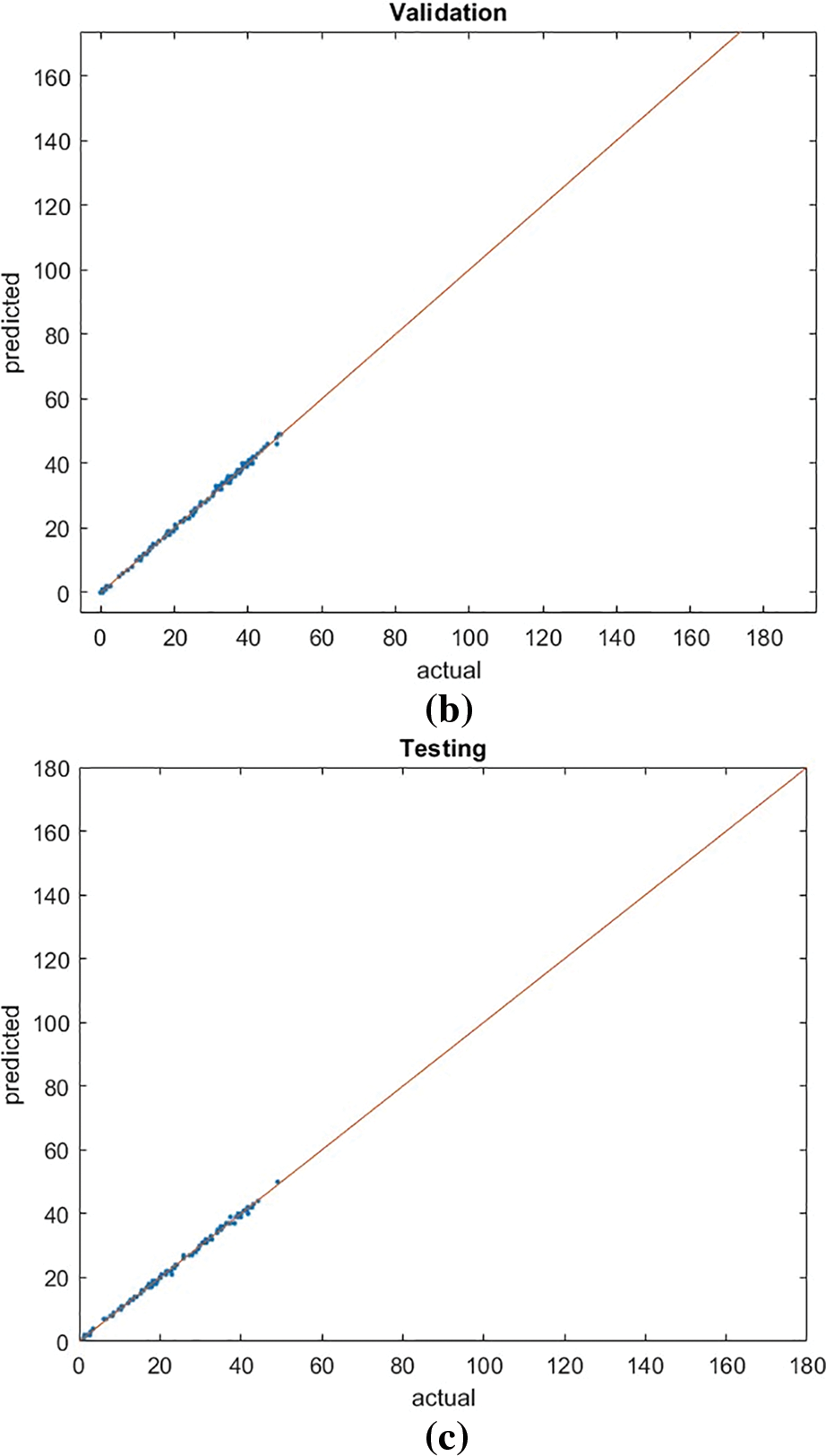
Figure 20: Grain orientation modeling. a) training, b) validation, c) testing

The orientation data of the EBSD figures is consolidated and randomized before being split into training (70%), validation (15%), and testing (15%) sets. The result of this neural network was not remarkably high, indicating RMSE, but instead accurate because RMSE is the traditional method for assessing the performance of the neural networks (NN); it is based on the error between the actual and the predicted value. The data is trained using an LSTM network comprising two layers with 50 and 20 neurons, respectively, subsequently connected to fully connected and regression layers. The settings for the network parameters are as follows:

•   MaxEpochs 500.

•   Gradient Threshold 1.

•   Initial Learn Rate 0.005.

•   Learn Rate Schedule Piecewise.

•   Learn Rate Drop Period 125.

•   Learn Rate Drop Factor 0.2.

The performance for training was recorded at 0.3188, for validation at 0.3181, and for testing at 0.3596.

6  Discussion

The primary aim of this research was to evaluate the SS316 material and its microstructural properties. Machine learning techniques were employed to predict future outcomes, demonstrating that these models could effectively interpret the arrangement of variables. The results showed that machine learning accurately captured the distribution of individual parameters, successfully replicating the grain pattern. However, the training data was limited due to a small number of experiments, which constrained the machine learning algorithm’s accuracy. Daily research faced challenges related to distortion and generating electron backscatter diffraction (EBSD) images, but even with a limited sample size, the concept was validated. Increasing the sample size will improve the system’s overall reliability and performance.

The study indicated that microstructure changes due to deformation, as evidenced by the varying intensities of grain orientation. Generally, grains reorient from 111 to 101 and 001 directions during rolling. At low temperatures (850°C), strain rate effects were minimal, whereas, at higher temperatures, grain orientation remained stable under high strain rates. A significant property change occurs when the strain rate decreases, suggesting either stability under high stress or the material’s ability to revert to its original state post-deformation. To fully grasp this behavior, it is crucial to analyze the microstructure at different stages of deformation, providing a temporal perspective on its evolution.

Utilizing deep learning, particularly Convolutional Neural Networks (CNNs), for grain orientation prediction offers significant advantages over traditional methods. CNNs can efficiently process high-dimensional image data, accurately capturing complex patterns in microstructural images. Once trained, CNN models can rapidly predict grain orientations, enabling real-time or near-real-time analysis and effectively scaling with large datasets. In contrast, traditional methods like EBSD require manual calculations and calibration, which are time-consuming and resource-intensive. The fast prediction capabilities of CNNs can enhance understanding of structure-property relationships, accelerate material discovery and optimization, and improve material performance in aerospace, automotive, and electronics industries.

7  Conclusion

The machine learning approach employed in this research demonstrated successful prediction of grain orientation post-deformation with satisfactory accuracy. These findings can inform the design of SS316 steel and other materials subjected to deformation and lay a strong foundation for using machine learning to predict grain orientation in more complex microstructures. Such advancements can aid engineers in developing more efficient and effective materials for various applications. However, a limitation lies in the EBSD images, where grain orientation resolution is influenced by the color differentiation in the image, making it difficult for the algorithm to distinguish between different orientations at small angles.

This study shows that grain orientation can be predicted using EBSD images without resorting to complex mathematical formulas, which are often time-consuming and error-prone. CNNs enhance the processing speed of EBSD images, providing a more efficient alternative to traditional mathematical models. Future research should explore broader deformation conditions, including different strain rates and temperatures, and incorporate data from diverse materials such as ceramics and polymers to improve the model’s applicability. Advanced CNN architectures like ResNet and DenseNet could further enhance image recognition capabilities, extending deep learning models’ predictive power to other materials and characterization techniques. This approach opens new possibilities for designing advanced materials with superior properties, driving innovation and progress in materials engineering.

Acknowledgement: Not applicable.

Funding Statement: The authors received no specific funding for this study.

Author Contributions: Conceptualization, Dhia K. Suker, and Ahmed R. Abdo; methodology, Dhia K. Suker, and Ahmed R. Abdo; experimental and modeling, Ahmed R. Abdo, and Dhia K. Suker; writing original draft preparation, Ahmed R. Abdo, and Dhia K. Suker; writing review and editing, Dhia K. Suker, and Khalid Abdulkhaliq M. Alharbi; supervision, Dhia K. Suker, and Khalid Abdulkhaliq M. Alharbi; funding acquisition, Dhia K. Suker, Ahmed R. Abdo, and Khalid Abdulkhaliq M. Alharbi. All authors reviewed the results and approved the final version of the manuscript.

Availability of Data and Materials: Data and materials will be available upon request.

Ethics Approval: Not applicable.

Conflicts of Interest: The authors declare that there are no conflicts of interest to report regarding the present study.

References

1. Y. Wang, H. Wang, and Z. Xin, “Efficient detection model of steel strip surface defects based on YOLO-V7,” IEEE Access, vol. 10, pp. 133936–133944, 2022. doi: 10.1109/ACCESS.2022.3230894. [Google Scholar] [CrossRef]

2. A. Agrawal, K. Gopalakrishnan, and A. Choudhary, “Materials image informatics using deep learning,” in Handbook on Big Data and Machine Learning in Physical Sciences, World Scientific, 2020, pp. 205–230. doi: 10.1142/9789811204555_0006. [Google Scholar] [CrossRef]

3. L. Belhaj and S. F. Fourati, “Systems modeling using deep elman neural network,” Eng. Technol. Appl. Sci. Res., vol. 9, no. 2, pp. 3881–3886, 2019. doi: 10.48084/etasr.2455. [Google Scholar] [CrossRef]

4. A. Agrawal and A. Choudhary, “Deep materials informatics: Applications of deep learning in materials science,” MRS Commun., vol. 9, no. 3, pp. 779–792, 2019. [Google Scholar]

5. Z. Ding, G. Zhu, and M. De Graef, “Determining crystallographic orientation via hybrid convolutional neural network,” Mater. Charact., vol. 178, 2021, Art. no. 111318. [Google Scholar]

6. Z. Ding, E. Pascal, and M. De Graef, “Indexing of backscatter diffraction using a convolutional neural network,” Acta Mater, vol. 199, pp. 370–382, 2021. [Google Scholar]

7. Oxford Instruments NanoAnalysis, “EBSD,” Oxford Instruments, 2024. Accessed: Jul. 1, 2024. [Online]. Available: https://nano.oxinst.com/products/ebsd/ [Google Scholar]

8. F. J. Humphreys, “Characterisation of fine-scale microstructures by electron backscatter diffraction (EBSD),” Scr. Mater., vol. 51, no. 8, pp. 771–776, 2004. [Google Scholar]

9. R. Liu, A. Agrawal, W. Liao, A. Choudhary, and M. De Graef, “Materials discovery: Understanding polycrystals from large-scale electron patterns,” in 2016 IEEE Int. Conf. Big Data (Big Data), IEEE, 2016, pp. 2261–2269. [Google Scholar]

10. D. Jha et al., “Extracting grain orientations from EBSD patterns of polycrystalline materials using convolutional neural network,” Microsc. Microanal., vol. 24, pp. 497–502, 2018. [Google Scholar] [PubMed]

11. C. Shu, Z. Xin, and C. Xie, “EBSD grain knowledge graph representation learning for material structure-property prediction,” in 6th China Conf. Knowl. Graph Seman. Comput., Springer, 2021, pp. 3–15. [Google Scholar]

12. D. K. Suker, T. A. Elbenawy, A. H. Backar, H. A. Ghulman, and M. W. Al-Hazmi, “Hot deformation characterization of AISI316 and AISI304 stainless steels,” Int. J. Metall. Met. Eng., vol. 17, pp. 1–14, 2017. [Google Scholar]

13. A. Hakimi, S. A. Monadjemi, and S. Setayeshi, “An introduction of a reward-based timeseries forecasting model and its application in predicting the dynamic and complicated behavior of the earth rotation (Delta-T Values),” Appl. Soft Comput, vol. 117, 2021, Art no. 108366. [Google Scholar]

14. B. Zahran, “Using neural networks to predict the hardness of aluminum alloys,” Eng. Technol. Appl. Sci. Res., vol. 5, no. 1, pp. 757–759, 2015. [Google Scholar]

15. I. Goodfellow, Y. Bengio, and A. Courville, Deep Learning. London, UK: MIT Press, 2016. [Google Scholar]

16. Y. Bengio, “Practical recommendations for gradient-based training of deep architectures,” in Neural Networks: Tricks of the Trade, G. Montavon, G. B. Orr, K. -R. Müller, Eds., 2nd ed. Berlin, Heidelberg: Springer, 2012, pp. 437–478. [Google Scholar]

17. M. J. Hasan, “Convolutional neural networks (CNNs),” 2020. Accessed: Jul. 1, 2024. [Online]. Available: https://jahidme.github.io/cnn/2020/04/13/cnn-intro/#/ [Google Scholar]

18. A. Goyal and Y. Bengio, “Inductive biases for deep learning of higher-level cognition,” 2021, arXiv:2011.15091. [Google Scholar]

19. A. R. Durmaz et al., “A deep learning approach for complex microstructure inference,” Nat. Commun., vol. 12, no. 1, 2021, Art no. 6272. [Google Scholar]

20. R. Ramprasad, R. Batra, G. Pilania, A. Mannodi-Kanakkithodi, and C. Kim, “Machine learning in materials informatics: Recent applications and prospects,” npj Comput. Mater., vol. 3, 2017, Art. no. 54. [Google Scholar]

21. R. Schwarzer, “An introduction to EBSD Backscatter Kikuchi Diffraction in the Scanning Electron Microscope (“BKD”, “ACOM/SEM”, “Orientation Microscopy”)” 2024. Accessed: Jun. 15, 2024. [Online]. Available: http://www.ebsd.info/index.html [Google Scholar]

22. S. Korpayev, M. Bayramov, S. Durdyev, and H. Hamrayev, “Characterization of three amu-darya basin clays in ceramic brick industry and their applications with brick waste,” Materials, vol. 14, no. 23, 2021, Art. no. 7471. doi: 10.3390/ma14237471. [Google Scholar] [CrossRef]