A Deep Transfer Learning Approach for Addressing Yaw Pose Variation to Improve Face Recognition Performance

1  Introduction

The identification of human faces [1] is crucial for distinguishing individuals from one another and identifying them for surveillance [2] applications. Intelligent system-based [3] detection and recognition are the two stages of FR for various applications, ranging from user authentication on devices to forensics [4] and intruder detection. Unlike fingerprint and signature authentication methods that require active user participation [5], FR identifies a person without direct interaction with the user. The advancement of video surveillance [6] has transformed the manual process into an interconnected intelligent control system [7]. This system discusses the phenomenon of FR in “Closed Circuit Television (CCTV)” images and future implementations of FR systems in live video streaming. Notably, there is a growing need for FR technology to identify faces in crowded areas, which plays a pivotal role in emerging research on FR systems to enhance biometric verification accuracy and efficiency while minimizing human errors and waiting time in queues.

The literature claims that factors such as pose variations [8], occlusions, facial expressions, and lighting conditions [9–12] can have an impact on the performance of FR algorithms. Conversely, research suggests that face datasets with greater pose variations [13] can strongly improve the performance of FR systems. Wu et al. developed a simulator and refiner module to generate frontal face images for the “three-dimensional (3D)” face images using the Deep Pose-Invariant Face Recognition Model [14]. To handle faces that have large pose variations, a novel method has been developed for learning pose-invariant feature embeddings [15]. This approach involves transferring the angular knowledge of frontal faces from the teacher network to the student network. Tao et al. proposed the Frontal-Centers Guided Loss (FCGFace) method to acquire highly discriminative features for face recognition. FCGFace achieves this by dynamically adjusting the distribution of profile face features and reducing the disparity between them and frontal face features at various stages of training, resulting in compact identity clusters [16]. Sengupta et al. presented a special data collection called “Celebrities in Frontal-Profile” that includes data from 500 different individuals with 4 images of profile faces in controlled and unconstrained environments [17].

In their study, Perez-Montes et al. introduced an evaluation subset containing various pose angles [18], ranging from 0° to 20°. They achieved a maximum verification score of 93.5% using the MobileFaceNet algorithm [19]. It is essential to train the model with various pose images to improve recognition in an unconstrained environment. This finding suggests that incorporating more pose variations in the dataset can help address the challenges posed by individuals facing the surveillance camera from different angles. In this study, the authors utilize a real-time dataset of 13 pose variations and attain a superior recognition rate for frontal-profile faces compared to advanced techniques. Furthermore, selecting the optimal feature vector size based on an examination of the Euclidean distance metric enhances the performance of the system.

2  Related Work

Addressing yaw pose variations is crucial for enhancing face recognition performance. Several studies have addressed this challenge using different methodologies. Pose-aware feature aggregation for FR has been introduced in recent work. This approach initially detects the facial features, predicts the pose of the face using a deep neural network, and subsequently extracts unique features using a model built on ResNet [20]. These features were aggregated using weighted feature maps from the different ResNet layers. The approach achieved an impressive accuracy of 96.91% when evaluated on the LFW dataset, covering a wide range of yaw angles from −90° to 90°. This research highlights the effectiveness of pose-aware feature aggregation in improving the FR across diverse pose variations. Naser et al. developed a system integrating “Multi-task Cascaded Convolutional Networks (MTCNN)”, FaceNet, and “Support Vector Classifier (SVC)” to detect faces with yaw pose variations from 0° to ±90°, achieving a high accuracy of 96.97% [21]. Gimmer et al. developed Syn-YawPitch, a 1000-identity dataset with different yaw-pitch angles and showed that pitch angles exceeding 30° significantly affect biometric performance [22]. The method proposed by Choi et al. leverages an angle-aware loss function inspired by ArcFace to provide a large margin for significantly rotated faces, ensuring better feature extraction for varying face angles and improving recognition accuracy [23].

The paper introduces the Large-Pose-Flickr-Faces Dataset (LPFF), a collection of 19,590 real large-pose face images designed to address the pose imbalance problem in current face generators. By integrating the LPFF dataset with existing datasets such as Flickr-Faces-HQ Dataset (FFHQ), a new dataset known as FFHQLPFF is created, which is further augmented by a horizontal flip to balance the pose distribution. To ensure a focus on large-pose data, the LPFF dataset is rebalanced by dividing it into subsets based on data densities rather than yaw angles. The “Efficient Geometry-aware (EG) 3D” face reconstruction model is utilized to extract camera parameters from the dataset. Although the LPFF dataset shows improvements, it still grapples with semantic attribute imbalances, such as the entanglement between smile-posture attributes [24].

The “Hypergraph De-deflection and Multi-task Collaborative Optimization (HDMCO)” method is a FR technique that employs advanced optimization for enhanced performance. It embeds hypergraphs in image decomposition to address pose deflection and extracts robust features using a feature-encoding method. In addition, HDMCO jointly optimizes tasks for improved recognition. Specifically, discrimination enhancement method is based on non-negative matrix factorization and hypergraph embedding, which extracts near-frontal images from pose-deflected images [25]. The “Two-Gradient Local Binary Pattern (TGLBP)”, designed for effective small-pose face recognition. This method achieves superior accuracy and robustness against noise. It consists of “Chinese Academy of. Sciences (CAS)-Pose, Expression, Accessory, and Lighting (PEAL)” face database, which comprises 99,450 face images of 595 Chinese men and 445 Chinese women, capturing diverse variations in terms of background, illumination, accessories, expressions, and gestures. Despite the encouraging outcomes demonstrated by the TGLBP algorithm, this study acknowledges the constraints it faces in addressing large-scale rotations in human faces [26].

3  Methodology

The proposed FR system is illustrated in Fig. 1. This section provides a detailed description of the method implemented for achieving pose-invariant FR. A key component of any FR system involves converting a raw image of a human face into a one-column dimensional vector, known as face feature embedding. Determining the optimal Euclidean distance threshold is crucial for establishing a decision boundary that distinguishes whether an individual belongs to the same identity or a different one. FaceNet utilizes a deep convolutional neural network, exploring two main architectures: the original Zeiler & Fergus-style [27] networks and the more recent Inception-type models. Specifically, the deep FR algorithm (without the transfer learning approach) uses an optimized Inception-v2 architecture with 164 layers. This architecture effectively selects the finest feature vector dimension, ensuring accurate identification of individuals across different yaw poses, as discussed in Section 4.

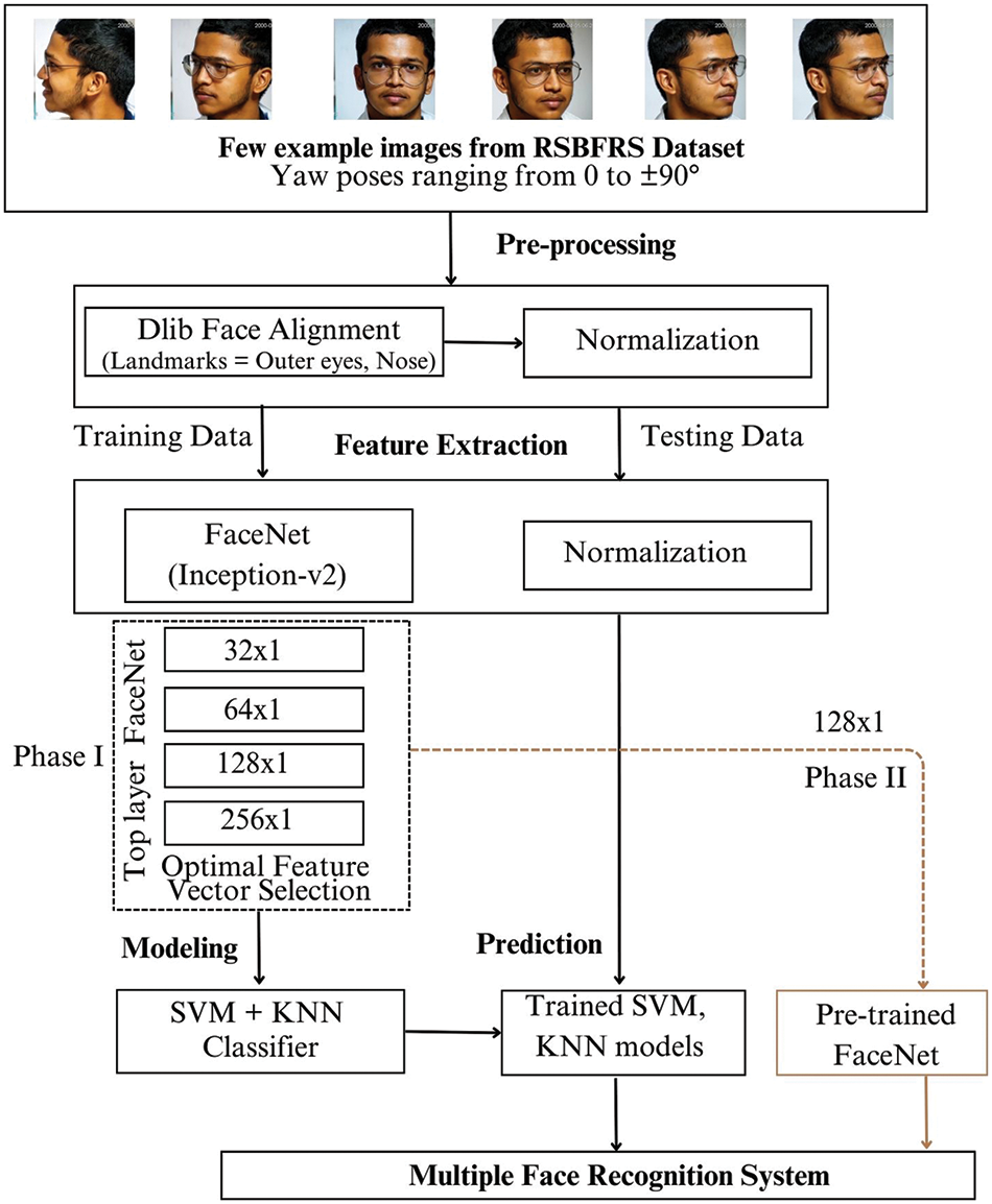
Figure 1: Proposed method for multiple FRs

3.1 Input CCTV Image Acquisition and the RSBFRS Database

A full-HD Dahua “Pan-Tilt-Zoom (PTZ)” camera was connected to a high-end graphics card-equipped workstation for edge computing [28]. This camera has a resolution of 2 megapixels and captures 25–30 frames per second. Data acquisition was performed for various pose angles ranging from −90° to +90° with one frontal face and 12 non-frontal-profile faces [29]. Consequently, the RSBFRS dataset [30] comprises of 8983 samples of 691 individuals, with each having 13 different pose images of size 1920 × 1080 pixels. This uniform diversity in the dataset makes it a unique dataset for addressing yaw poses. The training and test split ratio divided the training and validation datasets into 80:20 and later into 50:50 (RSBFRS data) throughout the process.

3.2 Face Detection and Dlib Face Alignment Technique

Before training the face recognition system, we performed Face Alignment and Resampling. The input images from both the RSBFRS and LFW databases were subjected to face alignment using the Dlib library. Following facial alignment, the images were resampled to a standardized size of 96 × 96 pixels using OpenCV. This normalization step ensures that the input data fed into the face recognition system have consistent size and alignment, thereby enabling accurate feature extraction and model training. Each participant contributed 13 pose-variation samples as input. The primary focus is to obtain a pose-invariant FR system, so the Dlib [28] open-source library provides useful information about facial landmarks, making the face alignment procedure easier. Dlib utilizes a pre-trained face detector consisting of a “Histogram of Oriented Gradients (HoG)” and a Linear SVM. HoG determines information regarding the texture and shape of facial images by calculating the distribution of gradient orientations in tiny regions of the image. This method focuses on specific facial features, such as the outer corners of the left and right eyes and the tip of the nose. These points aid in aligning faces with varying yaw angles. A linear SVM classifier was used to distinguish between the face landmarks and background regions based on HOG feature descriptors. The linear SVM algorithm determines the optimal hyperplane to divide positive (landmark) and negative (non-landmark) samples in the feature space. This is accomplished by mathematically addressing the optimization problem, as shown in Eq. (1).

minw,b12‖w‖2subject to yi(w.xi+b)≥1 for i=1,…,N(1)

where w is the weight vector, b is the bias term, xi is the feature vector for the ith sample, yi is the class label for landmark and N is the number of training samples. Hence, the Dlib detector detects the faces in a given image using landmark localization. These landmarks serve as reference points for subsequent tasks, such as face alignment, where the detected landmarks are used to normalize and align the face images. After detecting the face, each input image was passed through a face alignment block to resample into an image size of 96 × 96, followed by normalization.

3.3 Optimized FaceNet Architecture Details with the Tuning of Feature Vector Dimensions

In this section, we delve into feature extraction using the Inception-v2 network. The Inception architecture aims to identify the optimal sparse structure for a convolutional network and supplementing it with dense components to provide a c lose approximation. Fig. 2 illustrates a fundamental version of the inception module, where 1 × 1, 3 × 3, and 5 × 5 convolutional filters are applied to the input, followed by max pooling. The concatenated outputs from this module are then passed to the subsequent inception module.

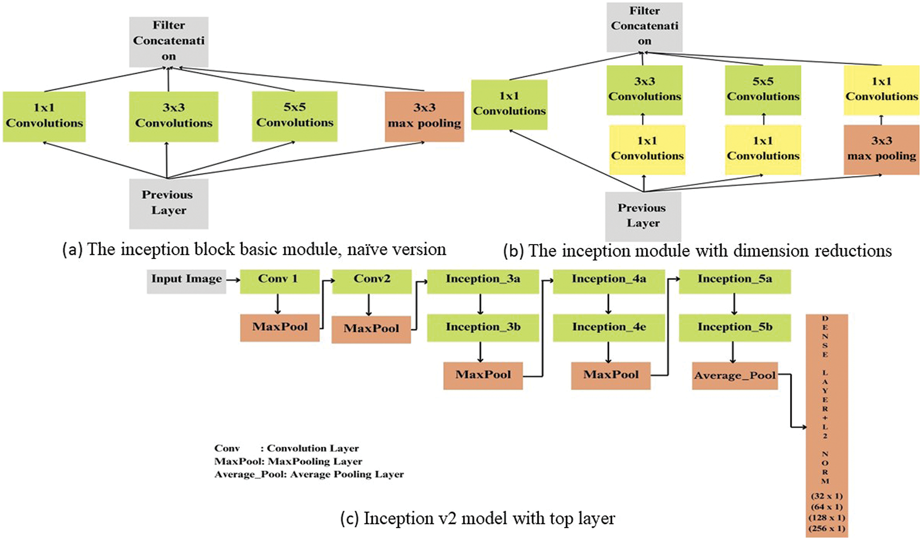
Figure 2: Inception-v2 architecture details

Generally, deep neural networks are expensive. Szegedy et al. [29] proposed a strategy to reduce operation costs by introducing a 1 × 1 convolution before the 3 × 3 and 5 × 5 convolutions, as depicted in Fig. 2b. Although counterintuitive, 1 × 1 convolutions are significantly more cost-effective than their larger counterparts (5 × 5 convolutions), and the smaller number of input channels also aids in cost savings. A 1 × 1 convolution was placed after the max pooling layer. The primary network layer implementation details of the inception module have been taken from the literature [31], focusing only on the top layer changes and optimization of the architecture using the “Root Mean Square Propagation (RMSProp)” optimizer. Optimization consists of L2 regularization by replacing the fixed learning rates with variable learning rates. Based on the average of the squared gradients over time, the RMSProp method adaptively adjusts the learning rate for each parameter. Consequently, the chosen learning rate was 0.0004 for fast convergence.

An input image of shape 96 × 96 × 3 is fed into the first convolution layer of the Inception-v2 module because the input size for “Neural Network4 (NN4)” is 96 × 96, followed by a max-pooling layer. Subsequently, two sets of inception modules with a down-sampling component named Inception 3a, Inception 3b, Inception 4a, and Inception 4e are connected; before the dense layer, two inception modules are added with an average pooling layer. When the receptive field is too small, the higher layers do not incorporate 5 × 5 convolutions, apart from the decreased input size. A dense layer follows the convolutional base with 128 hidden units, followed by an L2 normalization layer—these two outermost layers—are known as embedding layers of size 128 [32]. It employs the weights nn4.small, 2. v1 model, which was pretrained. Suppose the number of hidden neurons in a neural network is less than 16; in this case, it does not possess the potential to learn enough relevant patterns to differentiate between facial and non-facial features. Based on the analysis, if the neural network consists of more than 16 neurons, it performs better in classification problems. We plan to create dense units of sizes 32, 64, 128, and 256.

The modified 164-layered Inception-v2 architecture details are depicted in Fig. 2c. The architecture comprises convolutional layers, batch normalization, activation functions, max pooling, and local response normalization layers, which form the fundamental components of the initial network. We considered multiple filter sizes for each layer. The Inception-v2 model was utilized in two distinct phases. In the first phase, the entire Inception-v2 model was loaded with the corresponding weight file, and the model was trained for a publicly available dataset (LFW) and custom real-time data (RSBFRS). Once trained, all layers of the model, including those specific to different stages, such as inception 3a, 3b, 3c, 4a, 4e, 5a, and 5b, are frozen. Their weights remained unchanged during subsequent training, preserving the knowledge acquired from the initial training phase. Only the dense layer with dense unit 32 is further trained for all the input images, converted into feature vectors of size 32 × 1, and stored as a database. Similar operations were performed for the 64 × 1, 128 × 1, and 256 × 1. These features were then utilized for classification using SVM and KNN.

In the second phase, denoted as Phase II in Fig. 1, we aimed to reduce the training time and complexity, a pre-trained Inception-v2 model with a specific feature vector dimension of 128 × 1 was used to extract face features in live video streaming. The obtained face vector was then compared with the stored vector database with Euclidean distance as a metric able to recognize both known and unknown faces.

3.4 Triplet Loss

The selection of triplets plays a crucial role during the training process. These triplets should contain positive pairs (zia, zip) and negative pairs (zia, zin) that are challenging to distinguish, meaning that their difference in distance within the embedding space should be minimal, ideally less than the specified margin α. If the chosen triplets do not match this condition, the network may struggle to learn meaningful embedding. Therefore, in each training iteration, a new set of triplets must be chosen, depending on the embeddings obtained in the previous iteration. This iterative procedure ensures that the network consistently learns and acquires knowledge from data effectively. An anchor and positive image pair outputs a smaller value for triplet loss, thus forming the same identity. However, the anchor and negative image pairs have a higher triplet loss value, thus representing a different identity. The triplet-selection criteria are shown in Fig. 3.

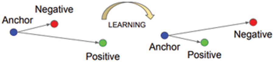
Figure 3: The triplet loss training concept

The embedding is given as f(z)∈Rd. It maps an image z into a d-dimensional Euclidean space and forces the embedding to reside on the surface of the d-dimensional hypersphere as ‖f(z)‖2 = 1. This study [33] proposed a loss to guarantee that a given image zia (anchor) of a particular person is closer to all other pictures zip (positive) of that person than it is to any image zin (negative) of a different person. Fig. 3 illustrates this. The expression for the triplet loss L [1] is given in Eqs. (2) and (3):

‖f(zia)−f(zip)‖22+α<‖f(zia)−f(zin)‖22(2)

∀(f(zia), f(zip), f(zin)∈τ(3)

α denotes the margin between positive and negative pairs. The τ set contains all possible triplets that appear in the training set and has a size of N. L is the quantity that is minimized and given as

L=‖f(zia)−f(zip)‖22−‖f(zia)−f(zin)‖22+α(4)

3.5 SVM + KNN Classification

The feature vectors extracted by Inception-v2 were then used as inputs to the SVM + KNN classifiers for face recognition. In a high-dimensional feature space, SVM is trained to differentiate the feature representations of distinct individuals, whereas KNN labels test samples according to the major class of their nearest neighbors. KNN classifies a data point by assigning it to the class that is most prevalent among its k closest neighbors, where k is a value determined by the user. Here we select, k = 5. This classifier uses a regularization parameter. This can be expressed mathematically as follows:

minw,b12‖w‖2+C∑i=1Nξi subject to yi(w.xi+b)≥1−ξi and ξi≥0 for i=1,…N(5)

where C is the regularization parameter. In summary, the proposed system initially uses Dlib to detect faces in an image and extract face landmarks (specifically, the outer eyes and nose tip) for integration with the feature extraction block. Then, a resampled face image of size 96 × 96 was passed through (Inception-v2) FaceNet to extract their embeddings. Finally, the vector of feature embeddings was classified using SVM + KNN to determine the identity of the detected face.

4  Results and Discussion

To implement this architecture in real-time scenarios, the open datasets LFW and RSBFRS (which contain 8983 images) were fed into the Inception-v2 model. After training with these datasets, each face image was transformed into vectors of dimensions 32 × 1, 64 × 1, 128 × 1, and 256 × 1. This system generates a vector of 128 points that represents a person’ s face and is effective for identifying similar faces. A feature vector of the identity is compared with each feature vector of the other identities. To identify known faces in the datasets, we developed a model that utilizes linear SVM and KNN to classify normalized face embeddings. This approach effectively distinguishes between vectors by training a linear SVM on face-embedding data, enabling accurate classification. The Euclidean distance was calculated for the feature vectors of the image pairs. Thus, recognition occurs. Further details of these results are provided below.

4.1 Experimental Setup for Data Collection and Database Used

Fig. 4 illustrates the experimental setup for RSBFRS data collection. This camera setup provides a unique advantage in that it allows individuals to be identified from a distance. The performance of the developed algorithm was assessed using two datasets, LFW [34] and RSBFRS. The developed algorithm is verified using the LFW dataset. The database consisted of 13,233 face images collected from the web of 1680 individuals for training and validation. Additionally, CCTV videos were created to investigate the challenge of recognizing faces in an unconstrained environment. The dataset comprises 700 videos.

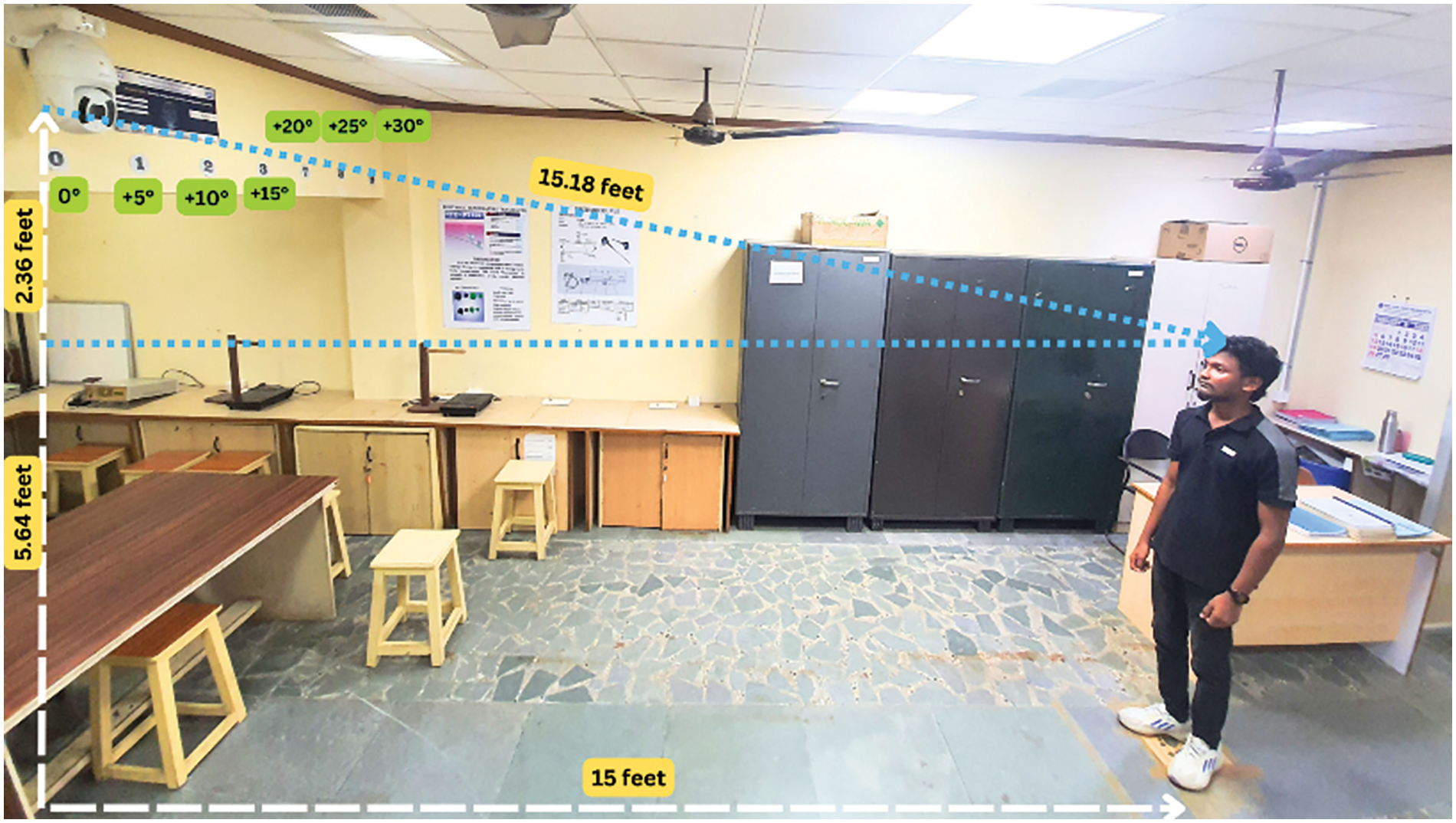
Figure 4: The complete setup for face data collection using the Dahua PTZ camera

The LFW dataset is widely utilized in FR research, with a primary focus on frontal poses. However, this dataset may lack diversity in terms of extreme yaw angles, potentially limiting the exposure of developed methods to challenging non-frontal poses and affecting their generalization to real-world scenarios with greater pose variations. The datasets used for evaluation may also exhibit some limitations and biases, particularly concerning the diversity of the represented yaw poses. Since the face data collection was conducted under constant illumination and lighting conditions, this is particularly relevant. The lack of diversity in yaw poses at certain angles and the uniform lighting conditions in the dataset pose significant limitations and biases for evaluation. In future work, addressing these issues by incorporating a more diverse range of yaw poses and capturing data under various lighting conditions will enhance the overall FR system performance. The RSBFRS dataset is collected at certain angles, and there might be a chance to omit angles from ±30° to ±90°. The yaw poses in the dataset are distributed as follows: To the right: +10, +30, +45, +60, and +90 degrees, To the left: −10, −30, −45, −60, and −90 degrees. Hence, certain yaw angles may be underrepresented, affecting the FR system performance for specific pose variations.

4.2 Results of Facial Alignment and Detection of Yaw Pose Images in the LFW and RSBFRS Datasets

As stated in Section 2, the preprocessing step is carried out consistently for all training and testing samples in the face detection module. Before modeling, the data undergoes preprocessing. Upon loading the database, Dlib and OpenCV execute the face detection process. Fig. 5a shows an example of an input face image from the LFW database. Fig. 5b illustrates the detection output, as shown in Fig. 5c. A resized image output of 96 × 96 pixels is displayed. Dlib utilizes the detected face points to resize and crop all input images to a standard dimension of 96 × 96 pixels, ensuring that facial images are transformed into a consistent size, disregarding the position of the key points on the face. It is important to normalize the phase-embedding vectors since they are typically measured using a distance metric.

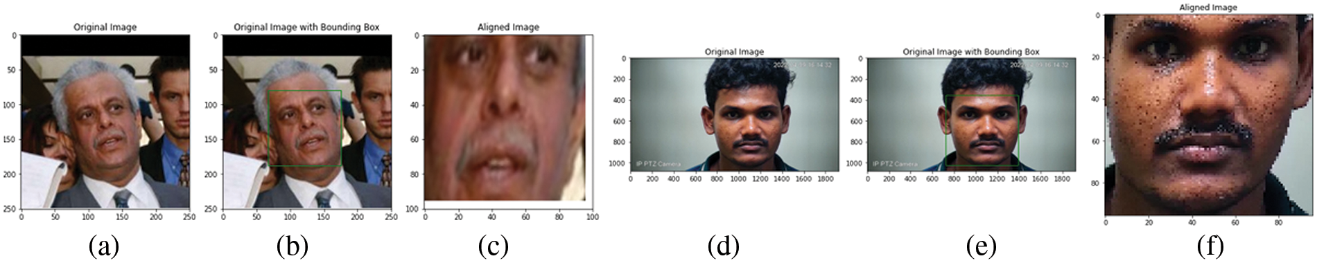
Figure 5: (a) Input face image from the LFW database, (b) output of face detection, (c) rescaled image (d) input CCTV image, (e) output window for face detection, (f) output rescaled image

4.3 Comparative Analysis of the Euclidean Distance for Different Yaw Poses

The output Euclidean distance values of the positive and negative image pairs to the number of dense units are given in Table 1. A single triplet image sample was verified on the LFW and RSBFRS databases.

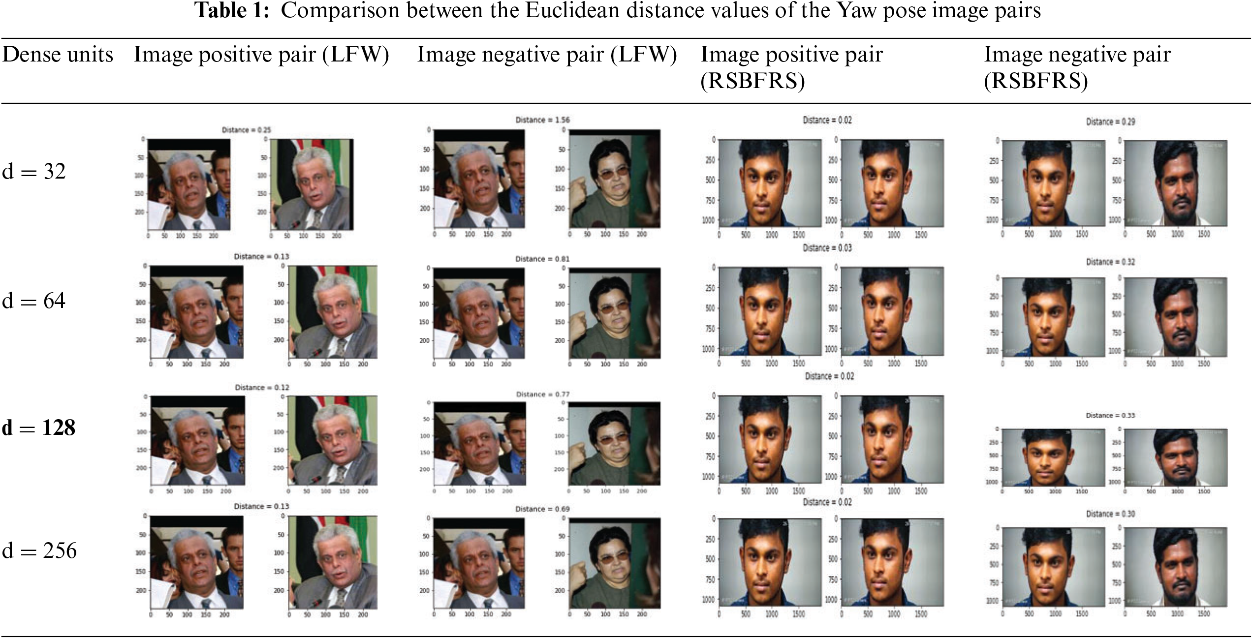
The number of dense layer units used can significantly affect its performance. Increasing the number of units improved the accuracy of the model. Simultaneously, the complexity of the model increases, which can lead to overfitting. On the other hand, decreasing the number of units can reduce the complexity of the model, but may decrease its accuracy. Thus, striking a balance between the number of units and the accuracy is crucial. The rows in Table 1 show the difference between the Euclidean distance values for image-positive and image-negative pairs from the LFW database for dense units d = 32, 64, 128, and 256. To select the most appropriate threshold value, it is necessary to evaluate the performance of face verification across a range of distance threshold values. The ground truth was compared to all embedding vector pairs with the same or different identities at a given threshold. For example, in the dense unit of 32, the positive and negative pairs of the image show distance values of 0.25 and 1.56, respectively. Hence, we computed the F1 score and accuracy for various distance thresholds ranging from 0.3 to 1, with an interval of 0.01. For each threshold value, we classified pairs of face embeddings as genuine (same identity) or impostor (different identity), based on whether the distance between the embeddings was below the threshold. We identified a threshold value that maximized the F1 score, indicating a balance between precision and recall. This threshold value ensures optimal performance in distinguishing genuine and impostor pairs.

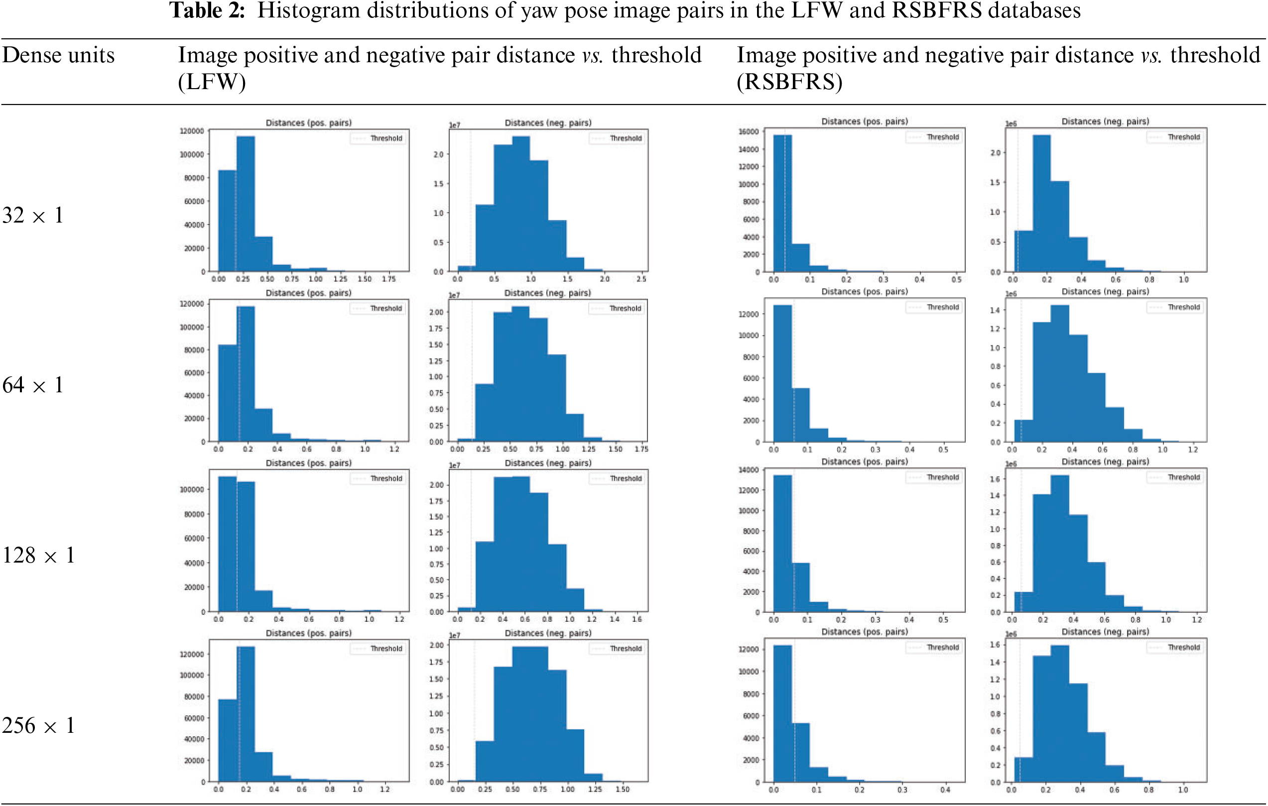
The LFW database has identified a threshold value from the first row of Table 1, which shows a value of 0.12 for the positive image pair. In the RSBFRS database, the dense unit 32 achieves a distance value of 0.02 and 0.29 for the positive and negative image pairs, respectively. The iterative process begins with a threshold value of 0.3 and continues until the optimal value is determined, as previously discussed. The maximum value for the distance threshold is 0.03, as shown in Table 1. After multiple iterations through each threshold value, the maximum F1 score was achieved at a threshold of 0.06. The results show that the dense unit of size 128 and the corresponding feature vector output of size 128 × 1 provide the minimum distance value of 0.12 for positive image pairs in the LFW database. Overall, this feature vector provides the minimum distance percentage for both positive and negative image pairs and can be considered the most suitable for facial recognition in yaw pose variations. The Table 2 histogram depicts the positive and negative pair distance distributions as well as the decision boundary. The superior performance of the network can be ascribed to the unique nature of these distributions. The 128 × 1 dimensional vector exhibits better distributions compared to the other cases, and all positive pairs groups contain notable outliers. As per the information in Table 1, a feature vector with a dimension of 64 has a significantly greater Euclidean distance. However, it is important to mention that the 128 × 1 dense unit produces a relatively lower distance value of 0.02 for similar images, which appears reasonable in comparison to other dimensions. The findings revealed that a feature vector size of 128 × 1 outperforms the other values.

Examine a face image measuring 1920 × 1080 pixels, which has been resized to 96 × 96 pixels and subsequently converted into 32 × 1, 64 × 1, and 128 × 1 feature points. To comprehend the disparity between 32 × 1 and 64 × 1 feature vectors with 128 points, consider the example depicted in Fig. 6. The values within the 32 × 1 feature vector range from approximately −0.304 to 0.340, exhibiting variation in magnitude with certain points close to zero and others demonstrating relatively larger values. The 64 × 1 feature vector encompasses a broader range than the 32 × 1 vector, spanning from approximately −0.393 to 0.317, showcasing increased variability within the dataset. The 128 × 1 feature vector indicates feature points ranging from approximately −0.190 to 0.203, revealing a narrower range of values compared to the 64 × 1 vector. This smaller spread in the 128 × 1 vector could be attributed to the higher density of data points falling within a more confined range, potentially resulting in a visually smaller appearance in the box and whisker plot.

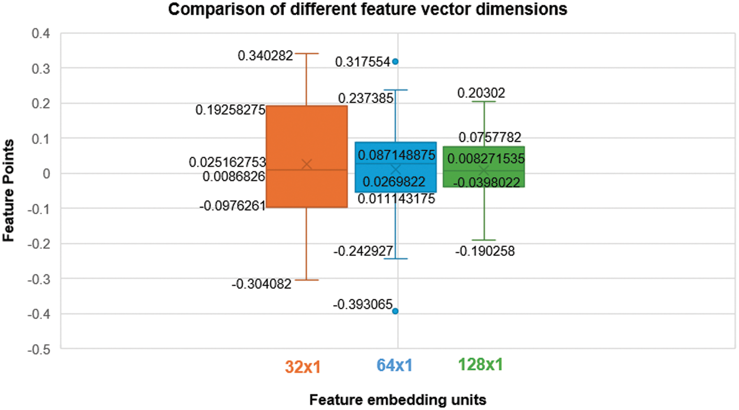
Figure 6: Plot for comparing different feature vectors of sizes 32 × 1, 64 × 1, and 128 × 1

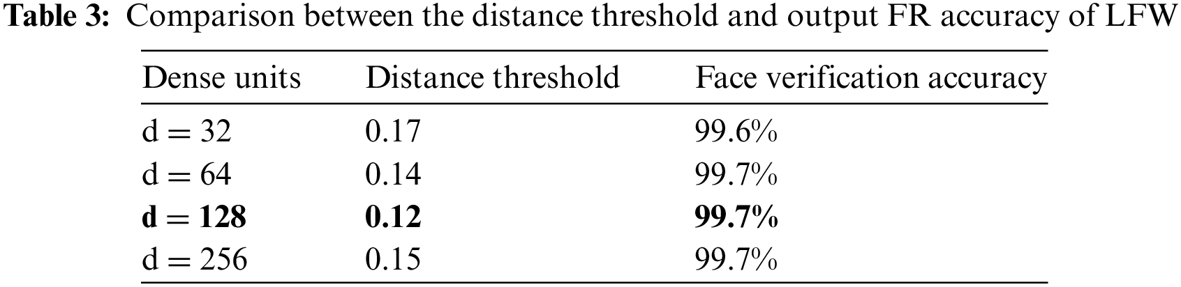
4.4 Comparison of Accuracy between Different Threshold Values and Dense Units

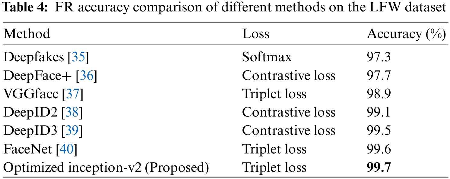
Using the LFW database, the performance of the modified inception architecture was evaluated for various dimensions of the feature vectors, d = 32, 64, 128, and 256. It achieved better results, with an FR accuracy of 99.7% for a minimum distance threshold value of 0.12, as shown in Fig. 7a. The details are presented in Table 3. During validation, at a distance threshold of 0.06 in the RSBFRS data, the FR system achieved an accuracy of 99.8%, as shown in Fig. 7b. This performance surpasses that of previous state-of-the-art methods compared in Table 4, and we obtained the highest FR accuracy. The metric used for calculating the recognition accuracy was computed using Eq. (6). Similarly, the classification accuracy was computed using Eqs. (7) and (8). Let ytrain and ytest be the actual labels for the training and test sets respectively. y^SVM and y^KNN are the predicted labels, Ntest is the number of samples in the test set. The classification accuracy for the SVM and KNN for the test set can be calculated as:

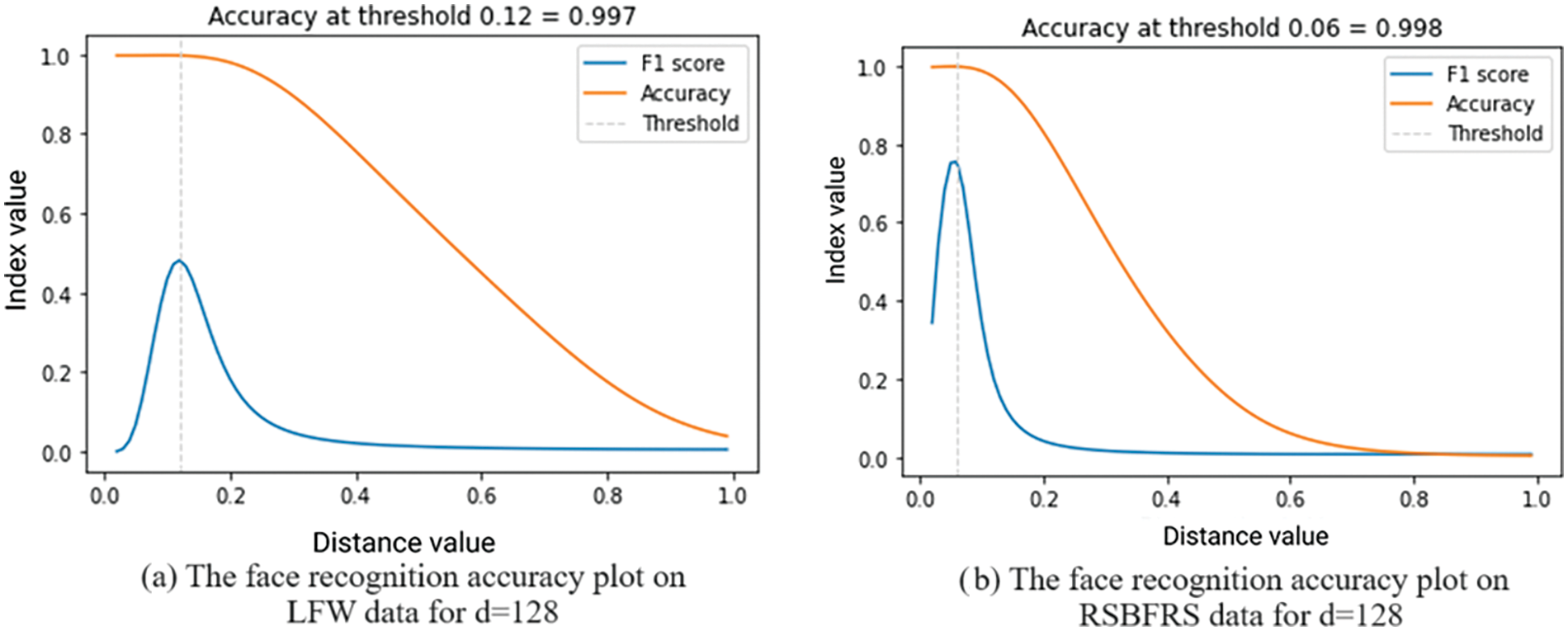
Figure 7: Plot of the highest FR accuracy, F1 score vs. distance threshold of the Inception-v2 model

4.5 Comparison of Classification Accuracy for Different Feature Vector Values

To achieve a higher classification accuracy, the LFW dataset was split into training and testing data at an 80:20 ratio. The accuracy can be further improved by incorporating additional features. The step-by-step progress in classification accuracy using the SVM and KNN techniques with the Inception-v2 model is shown in Table 5. Among these approaches, the FaceNet + KNN method achieved the highest accuracy of 87.71% for d = 256. The RSBFRS dataset was split into two parts. Half of the data were used to train the SVM and KNN classifiers, and the other half were used for testing. Table 5 shows the accuracy of the SVM and KNN classification techniques. The FaceNet + KNN classification method achieves the highest accuracy of 99.44% when the output dimension is 128 × 1. Therefore, it can be concluded from the table that feature vectors of sizes 64 and 128 provided better classification results than those of the other dimensions. In addition, a vector size of 128 yielded a lower Euclidean distance for positive image pairs, thereby improving the classification rate. According to the analysis, the optimal feature vector size was 128 × 1.

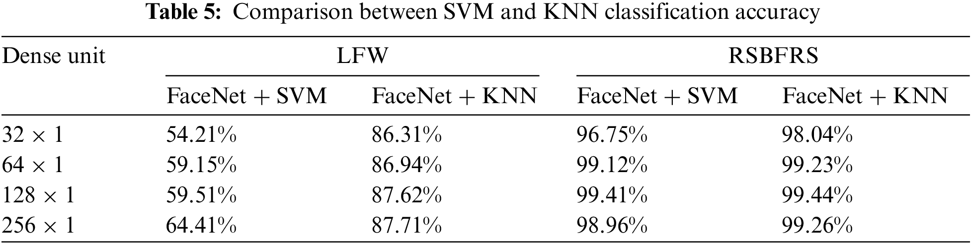
In Table 5, the significant disparities in classification accuracy between the LFW and RSBFRS datasets can be attributed to several factors. One of the key factors is that the RSBFRS has uniform diversity in yaw pose images in the database for 691 individuals with 1920 × 1080 resolution. Despite the smaller number of images in the RSBFRS dataset, it exhibits better class separability and reduced data imbalance compared to the LFW dataset. SVM and KNN classifiers performed optimally when the classes were well-separated and balanced. The RSBFRS dataset, which focuses on yaw pose variations, provides a more balanced representation of different classes, facilitating a better classification performance. The LFW dataset contains yaw pose face data. The dataset includes images with a few yaw angles and 250 × 250 resolution, allowing for the study of face recognition across different head orientations. The maximum angle of the face poses in the LFW dataset is not explicitly mentioned in the LFW database repository. However, the RSBFRS dataset introduced in our work encompasses a broader range of yaw pose variations, capturing facial images under diverse conditions. The trained model performed adequately on the LFW dataset with similar frontal faces, and its performance degraded significantly when applied to datasets with yaw pose variations. This advantage in class separability and reduced data imbalance in the RSBFRS dataset allows SVM and KNN classifiers to make more accurate distinctions between classes, resulting in higher classification accuracy compared to the LFW dataset.

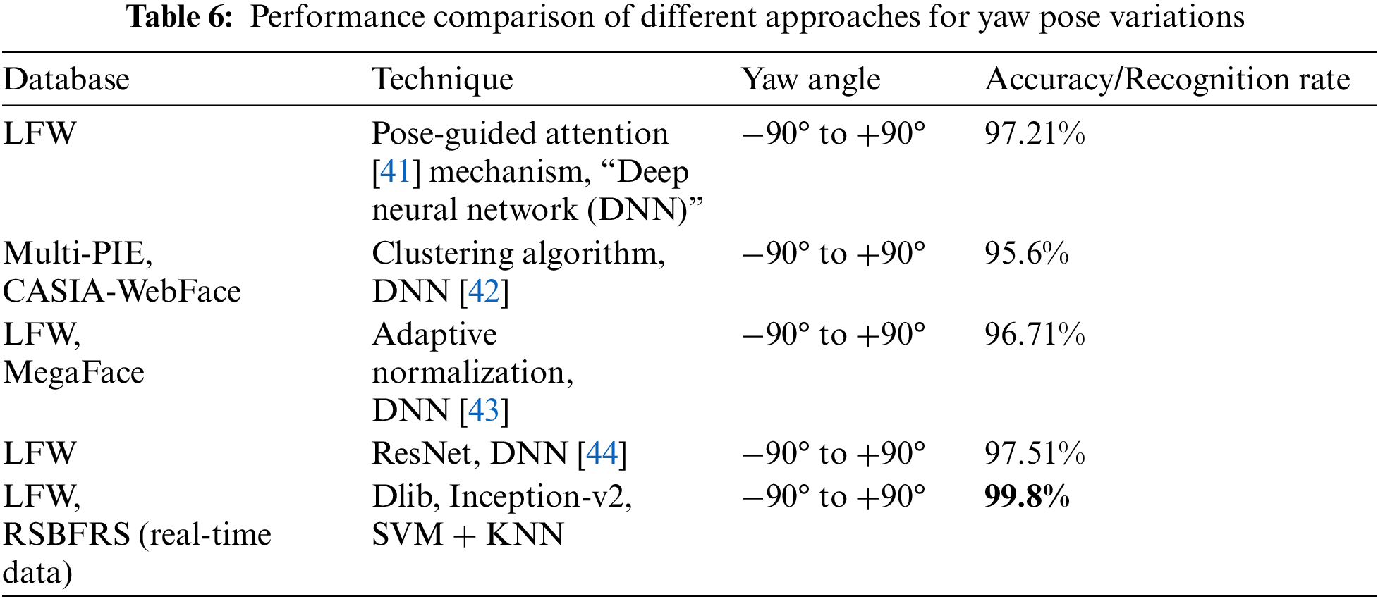
The focus of our study lies in investigating a substantial number of pose variation samples, positioning it as a pioneering approach for pose-invariant recognition. A comparison of performance is illustrated in Table 6. The developed inception model underwent rigorous training using pose variation samples from the RSBFRS dataset. This method cannot be contrasted with pose variant models, 3D models, and synthetic data generation techniques. The main objective of this research is to tackle the challenge of yaw-pose variation without employing synthetic data. The proposed approach consistently achieves a higher level of accuracy than previous techniques, as shown in Table 6, across a range of pose angles. It offers a comprehensive evaluation of the proposed approach in comparison to existing methods across various databases and yaw-angle ranges. The effectiveness of each method was quantitatively measured in terms of accuracy or recognition rate, providing insight into their relative strengths in dealing with non-frontal poses. As a result, this approach emerges as a well-suited solution for facial recognition with pose variations.

4.6 Limitations and Practical Applications

Although the proposed approach demonstrates promising results in addressing yaw pose variations and enhancing face recognition accuracy, several limitations should be addressed. The effectiveness of this approach may be influenced by the size of the training dataset used. Although the RSBFRS dataset used in this study contains a substantial number of images with yaw pose variations, it can be improved with a higher number of images. The reliance on pre-trained models, such as the Inception-v2 architecture, may introduce limitations related to model generalization and adaptation to specific domains or datasets. The performance of this approach may be sensitive to environmental factors such as lighting conditions and camera angles. The computational requirements of this approach, particularly during the training and inference stages, may pose limitations in resource-constrained environments or real-time applications.

The proposed approach holds significant potential for practical applications in real-world scenarios, especially in improving the functionality of facial recognition systems when dealing with challenging conditions characterized by non-frontal poses. In public places and crowded environments, accurately identifying individuals in non-frontal positions enhances public safety and security measures. Security personnel can efficiently identify individuals of interest and respond to potential threats more effectively, thereby contributing to overall public safety. Additionally, in access control systems utilized in workplaces, educational institutions, or residential complexes, the proposed approach can streamline the authentication process by accurately confirming the identities of individuals, regardless of their yaw pose.

5  Conclusion

This study systematically investigates the influence of yaw pose variation on the accuracy of facial recognition systems. We developed a robust solution to detect faces ranging from 0° to ±90°. Our approach, which integrates Dlib, FaceNet, and SVM + KNN, outperforms the existing methods. This method achieved a maximum recognition accuracy of 99.8% for RSBFRS CCTV data, with a minimum Euclidean distance value of 0.06. Similarly, the LFW data show a 99.7% recognition accuracy for a 0.12 distance threshold, confirming its ability to handle yaw pose variations better than existing approaches. We found that a feature vector dimension of 128 × 1 was optimal for both the positive and negative yaw image pairs. Furthermore, the supervised learning models, SVM and KNN, achieved a maximum classification accuracy of 87.71% for the LFW benchmark dataset and 99.44% for the real-time RSBFRS database. With the inclusion of 12 significant yaw pose variation images, the FR performance was improved with reduced computation time, making the system more efficient and accurate in a crowded environment. The FR system effectively recognizes faces from different angles (yaw positions). To further improve the accuracy rate, future works can focus on several factors. Expanding the RSBFRS dataset to include more real-time yaw pose image pairs beyond ±90° for all the individuals, ensures the uniformity between samples to create a more consistent and representative training dataset. Also, the addition of ear contours/features in the Dlib module could further improve recognition performance in yaw poses. This approach demonstrated significant accuracy compared to most known baseline methods, highlighting the potential use of a pose-invariant FR system in surveillance applications.

Acknowledgement: The authors extend their gratitude to the Board of Research in Nuclear Sciences (BRNS) for their support. Additionally, we appreciate the assistance from SRM Institute of Science and Technology, Kattankulathur, Chennai, for providing essential real-time data required for this research.

Funding Statement: The authors received funding for the project, excluding research publication, from the Board of Research in Nuclear Sciences (BRNS) under Grant Number 59/14/05/2019/BRNS.

Author Contributions: Conceptualization: M. Jayasree, K. A. Sunitha; Methodology: M. Jayasree, K. A. Sunitha; Software: M. Jayasree; Validation: M. Jayasree, K. A. Sunitha, A. Brindha, Punna Rajasekhar, G. Aravamuthan; formal analysis: K. A. Sunitha, Punna Rajasekhar, G. Aravamuthan, G. Joselin Retnakumar; investigation: K. A. Sunitha, Punna Rajasekhar, G. Aravamuthan; resources: M. Jayasree, K. A. Sunitha, A. Brindha, Punna Rajasekhar, G. Aravamuthan, G. Joselin Retnakumar; data Creation: M. Jayasree, K. A. Sunitha, A. Brindha, G. Joselin Retnakumar; writing and original draft preparation: M. Jayasree, K. A. Sunitha; supervision: K. A. Sunitha. All authors reviewed the results and approved the final version of the manuscript.

Availability of Data and Materials: The datasets generated during and/or analyzed during the current study are not publicly available because data involving human research participants may present a risk of reidentification if shared openly.

Conflicts of Interest: The authors declare that they have no conflicts of interest to report regarding the present study.

References

1. W. Ali, W. Tian, S. U. Din, D. Iradukunda, and A. A. Khan, “Classical and modern face recognition approaches: A complete review,” Multimed. Tools Appl., vol. 80, no. 3, pp. 4825–4880, 2021. doi: 10.1007/s11042-020-09850-1. [Google Scholar] [CrossRef]

2. N. K. Mishra, M. Dutta, and S. K. Singh, “Multiscale parallel deep CNN (mpdCNN) architecture for the real low-resolution face recognition for surveillance,” Image Vis. Comput., vol. 115, no. 5, pp. 104290, 2021. doi: 10.1016/j.imavis.2021.104290. [Google Scholar] [CrossRef]

3. S. Gupta, K. Thakur, and M. Kumar, “2D-human face recognition using SIFT and SURF descriptors of face’ s feature regions,” Vis. Comput., vol. 37, no. 3, pp. 447–456, 2021. doi: 10.1007/s00371-020-01814-8. [Google Scholar] [CrossRef]

4. S. M. La Cava, G. Orrù, M. Drahansky, G. L. Marcialis, and F. Roli, “3D face reconstruction: The road to forensics,” ACM Comput. Surv., vol. 56, no. 3, pp. 1–38, 2023. [Google Scholar]

5. C. W. Lien and S. Vhaduri, “Challenges and opportunities of biometric user authentication in the age of IoT: A survey,” ACM Comput. Surv., vol. 56, no. 1, pp. 1–37, 2023. [Google Scholar]

6. M. Obayya et al., “Optimal deep transfer learning based ethnicity recognition on face images,” Image Vis. Comput., vol. 128, pp. 104584, 2022. [Google Scholar]

7. R. Ullah et al., “A real-time framework for human face detection and recognition in cctv images,” Math. Probl. Eng., vol. 2022, no. 2, pp. 1–12, 2022. doi: 10.1155/2022/3276704. [Google Scholar] [CrossRef]

8. C. Wu and Y. Zhang, “MTCNN and FACENET based access control system for face detection and recognition,” Autom. Control Comput. Sci., vol. 55, no. 1, pp. 102–112, 2021. doi: 10.3103/S0146411621010090. [Google Scholar] [CrossRef]

9. A. Koubaa, A. Ammar, A. Kanhouch, and Y. AlHabashi, “Cloud versus edge deployment strategies of real-time face recognition inference,” IEEE Trans. Netw. Sci. Eng., vol. 9, no. 1, pp. 143–160, 2021. doi: 10.1109/TNSE.2021.3055835. [Google Scholar] [CrossRef]

10. T. H. Tsai and P. T. Chi, “A single-stage face detection and face recognition deep neural network based on feature pyramid and triplet loss,” IET Image Process., vol. 16, no. 8, pp. 2148–2156, 2022. doi: 10.1049/ipr2.12479. [Google Scholar] [CrossRef]

11. Z. Song, K. Nguyen, T. Nguyen, C. Cho, and J. Gao, “Spartan face mask detection and facial recognition system,” Healthcare, vol. 10, no. 6, pp. 87, 2022. doi: 10.3390/healthcare10010087. [Google Scholar] [PubMed] [CrossRef]

12. U. Jayaraman, P. Gupta, S. Gupta, G. Arora, and K. Tiwari, “Recent development in face recognition,” Neurocomputing, vol. 408, no. 1–3, pp. 231–245, 2020. doi: 10.1016/j.neucom.2019.08.110. [Google Scholar] [CrossRef]

13. M. Joseph and K. Elleithy, “Beyond frontal face recognition,” IEEE Access, vol. 11, pp. 26850–26861, 2023. doi: 10.1109/ACCESS.2023.3258444. [Google Scholar] [CrossRef]

14. H. Wu, J. Gu, X. Fan, H. Li, L. Xie and J. Zhao, “3D-guided frontal face generation for pose-invariant recognition,” ACM Trans. Intell. Syst Technol., vol. 14, no. 2, pp. 1–21, 2023. doi: 10.1145/3572035. [Google Scholar] [CrossRef]

15. Z. Zhang, Y. Chen, W. Yang, G. Wang, and Q. Liao, “Pose-invariant face recognition via adaptive angular distillation,” presented at the AAAI Conf. Artif. Intell., 2022, pp. 3390–3398. doi: 10.1609/aaai.v36i3.20249. [Google Scholar] [CrossRef]

16. Y. Tao, W. Zheng, W. Yang, G. Wang, and Q. Liao, “Frontal-centers guided face: Boosting face recognition by learning pose-invariant features,” IEEE Trans. Inf. Forensics Secur., vol. 17, pp. 2272–2283, 2022. doi: 10.1109/TIFS.2022.3183410. [Google Scholar] [CrossRef]

17. S. Sengupta, J. C. Chen, C. Castillo, V. M. Patel, R. Chellappa and D. W. Jacobs, “Frontal to profile face verification in the wild,” presented at the IEEE Winter Conf. Appl. Comput. Vis. (WACVLake Placid, NY, USA, Mar. 7–9, 2016, pp. 1–9. [Google Scholar]

18. A. S. Sanchez-Moreno, J. Olivares-Mercado, A. Hernandez-Suarez, K. Toscano-Medina, G. Sanchez-Perez and G. Benitez-Garcia, “Efficient face recognition system for operating in unconstrained environments,” J. Imaging, vol. 7, no. 9, pp. 161, 2021. doi: 10.3390/jimaging7090161. [Google Scholar] [PubMed] [CrossRef]

19. Y. V. Kale, A. U. Shetty, Y. A. Patil, R. A. Patil, and D. V. Medhane, “Object detection and face recognition using yolo and inception model,” presented at the Int. Conf. Adv. Netw. Technol. Intell. Comput., 2021, pp. 274–287. [Google Scholar]

20. W. C. Lin, C. T. Chiu, and K. C. Shih, “RGB-D based pose-invariant face recognition via attention decomposition module,” presented at the IEEE Int. Conf. Acoust. Speech Signal Process (ICASSP2023, pp. 1–5. [Google Scholar]

21. O. A. Naser et al., “Investigating the impact of yaw pose variation on facial recognition performance,” Adv. Artif. Intell. Mach. Learn., vol. 3, no. 2, pp. 62, 2019. [Google Scholar]

22. M. Grimmer, C. Rathgeb, and C. Busch, “Pose impact estimation on face recognition using 3D-aware synthetic data with application to quality assessment,” IEEE Trans. Biom. Behav. Identity Sci., vol. 6, no. 2, pp. 209–218, 2024. [Google Scholar]

23. J. Choi, Y. Kim, and Y. Lee, “Robust face recognition based on an angle-aware loss and masked autoencoder pre-training,” presented at the IEEE Int. Conf. Acoust. Speech Signal Process (ICASSP2024, pp. 3210–3214. [Google Scholar]

24. Y. Wu, J. Zhang, H. Fu, and X. Jin, “LPFF: A portrait dataset for face generators across large poses,” presented at the IEEE/CVF Int. Conf. Comput. Vis. (ICCV2023, pp. 20327–20337. [Google Scholar]

25. X. Fan, M. Liao, L. Chen, and J. Hu, “Few-shot learning for multi-POSE face recognition via hypergraph de-deflection and multi-task collaborative optimization,” Electronics, vol. 12, no. 10, pp. 2248, 2023. doi: 10.3390/electronics12102248. [Google Scholar] [CrossRef]

26. H. Qu and Y. Wang, “Application of optimized local binary pattern algorithm in small pose face recognition under machine vision,” Multimed. Tools Appl., vol. 81, no. 20, pp. 29367–29381, 2022. doi: 10.1007/s11042-021-11809-9. [Google Scholar] [CrossRef]

27. C. Szegedy, V. Vanhoucke, S. Ioffe, J. Shlens, and Z. Wojna, “presented at the IEEE Conf. Comput. Vis. Pattern Recognit. (CVPRBoston, MA, USA, 2016, pp. 2818–2826. [Google Scholar]

28. S. R. Boyapally and K. P. Supreethi, “Facial recognition and attendance system using dlib and face recognition libraries,” 2021 Int. Res. J. Modernization Eng. Technol. Sci., vol. 3, no. 1, pp. 409–417, 2021. [Google Scholar]

29. C. Szegedy et al., “Going deeper with convolutions,” presented at the IEEE Conf. Comput. Vis. Pattern Recognit. (CVPRBoston, MA, USA, 2015, pp. 1–9. [Google Scholar]

30. M. Jayasree, K. A. Sunitha, A. Brindha, P. Rajasekhar, and G. Aravamuthan, “BoundNet: Pixel level boundary marking and tracking of instance video objects,” presented at the 3rd Int. Conf. Emerg. Technol. (INCETBelgaum, India, 2022, pp. 1–6. [Google Scholar]

31. K. Q. Weinberger, J. Blitzer, and L. Saul, “Distance metric learning for large margin nearest neighbor classification,” Adv. Neur. Inf. Process Syst., vol. 18, pp. 1473–1480, 2005. [Google Scholar]

32. G. B. Huang, M. Mattar, T. Berg, and E. Learned-Miller, “Labeled faces in the wild: A database forstudying face recognition in unconstrained environments,” in Workshop Faces'Real-Life' Images: Detecti, Alignm, and Recogniti, Erik Learned-Miller and Andras Ferencz and Frédéric Jurie, Marseille, France, 2008. [Google Scholar]

33. Y. Taigman, M. Yang, M. Ranzato, and L. Wolf, “DeepFace: Closing the gap to human-level performance in face verification,” presented at the IEEE Conf. Comput. Vis. Pattern Recognit. (CVPRBoston, MA, USA, 2014, pp. 1701–1708. [Google Scholar]

34. D. Yi, Z. Lei, S. Liao, and S. Z. Li, “Learning face representation from scratch,” arXiv preprint arXiv:1411.7923, 2014. [Google Scholar]

35. O. Parkhi, A. Vedaldi, and A. Zisserman, “Deep face recognition,” presented at the Brit. Mach. Vis. Conf. (BMVCSwansea, UK, 2015. [Google Scholar]

36. Y. Sun, Y. Chen, X. Wang, and X. Tang, “Deep learning face representation by joint identification-verification,” Adv. Neur. Inf. Process Syst., vol. 27, pp. 1988–1996, 2014. [Google Scholar]

37. H. Wang et al., “Cosface: Large margin cosine loss for deep face recognition,” presented at the IEEE Conf. Comput. Vis. Pattern Recognit. (CVPRSalt Lake City, UT, USA, 2018, pp. 5265–5274. [Google Scholar]

38. Y. Sun, X. Wang, and X. Tang, “Deeply learned face representations are sparse, selective, and robust,” presented at the IEEE Conf. Comput. Vis. Pattern Recognit. (CVPRBoston, MA, USA, 2015, pp.2892–2900. [Google Scholar]

39. Y. Sun, D. Liang, X. Wang, and X. Tang, “DeepID3: Face recognition with very deep neural networks,” arXiv preprint arXiv:1502.00873, 2015. [Google Scholar]

40. F. Schroff, D. Kalenichenko, and J. Philbin, “FaceNet: A unified embedding for face recognition and clustering,” presented at the IEEE Conf. Comput. Vis. Pattern Recognit. (CVPRBoston, MA, USA, 2015, pp. 815–823. [Google Scholar]

41. J. Kaur, A. Sharma, and A. Cse, “Performance analysis of face detection by using Viola-Jones algorithm,” Int. J. Comput. Intell. Res., vol. 13, no. 5, pp. 707–717, 2017. [Google Scholar]

42. M. D. Zeiler and R. Fergus, “Visualizing and understanding convolutional networks,” presented at the13th Europe. Conf. Comput. Vis. (ECCVZurich, Switzerland, Sep. 6–12, 2014, pp. 818–833. [Google Scholar]

43. W. Zhao, T. Ma, X. Gong, B. Zhang, and D. Doermann, “A review of recent advances of binary neural networks for edge computing,” IEEE J. Miniaturization Air Space Syst., vol. 2, no. 1, pp. 25–35, 2020. doi: 10.1109/JMASS.2020.3034205. [Google Scholar] [CrossRef]

44. D. Manju and V. Radha, “A novel approach for pose invariant face recognition in surveillance videos,” Procedia Comput. Sci., vol. 167, no. 8, pp. 890–899, 2020. doi: 10.1016/j.procs.2020.03.428. [Google Scholar] [CrossRef]