Importance-Weighted Transfer Learning for Fault Classification under Covariate Shift

1  Introduction

Data-focused fault detection in industrial process has been heavily researched in the past few years, especially for plant-wide nonlinear chemical processes [1–9]. However, most of the related papers are focused on fault detection in a single working condition. Since traditional machine learning algorithms cannot cope with unknown input data, these methods often perform very poorly with different test samples, so there is a great need in industry for learning models that can learn from many different datasets for different working conditions [10]. This drawback restricted the effectiveness of fault detection algorithms for nonlinear multi-mode processes. It is essential to propose some new methods to better solve the problem of model transfer under unknown operating conditions or drift of operating conditions over time.

The actual industrial process usually runs in multiple operating modes [11] because of raw material fluctuations, seasonal changes in market demand, etc. For large-scale multi-mode industrial fault detection, the traditional machine learning-based fault detection algorithms cannot detect the drift of the process working conditions in time, which may lead effect and performance of the pre-designed fault detection algorithm to continually decline over time. On the other hand, fault detection in multi-mode chemical processes is usually achieved based on model recognition or model division. A mathematical model is established based on historical process data to obtain the monitoring indicators of each model of the multi-model process, and then determine whether the fault has occurred based on the monitoring indicators, thus issuing alerts in time to avoid serious accidents.

In the existing literature, it is assumed that there is no significant drift in operating conditions, and the fluctuation characteristics of process variables are stationary sequences (such as Gaussian distribution, etc.). However, in the actual industrial production environment, the conditions frequently change during the accumulated long-term operation, which would lead to certain drifts in the probable distributions of processing variables in the process. On the other hand, since the dynamic characteristics are determined by the mechanism of the actual production process, the nonlinear dynamic connection between the process variables and the system output usually does not change significantly. It is assumed that the training and testing data have the same input distribution, and a majority of traditional machine learning based methods could not work effectively under covariate shift. It could be solved by reducing the differentiation of the distribution of the training and testing data [12–19].

The existing literature regarding fault classification in nonlinear multi-mode processes usually does not consider the system operating conditions or the time-varying drift in terms of fault characteristics. The operation-condition ranges of the process system plants are assumed to be within the historical operation-condition ranges. In other words, they assume that there are no unknown operation conditions during the verification of fault classification in multi-mode processes. However, these assumptions are unreasonable for the actual industrial chemical process, because the data sample distributions of the training and testing dataset may not be perfectly consistent, which is due to the change of working conditions. And data characteristics can be changed due to fluctuations of raw materials. In addition, conventional data-driven methods work under the assumption that the dataset used for model training is sufficient, but the effective information or knowledge available in the actual production process usually is not sufficient to train the fault classification model. Therefore, it is significant to introduce the transfer learning [20] to the fault classification in the nonlinear multi-mode process. Transfer learning is a reliable method to solve the issue of deficiency data, and it utilizes the existing data or knowledge in historical scenes to assist the training process of the model [21]. In this study, the concept of covariate shift [22] in the transfer learning is introduced, and the importance-weight sampling is carried out. The contribution in this study can be summarized as:

1) This paper focuses on the application of covariate shifts for the industrial-process fault detection and classification. We introduced a practical reweighting method (importance weighting) [23], which can be formally proven that this approach is theoretically reliable [24].

2) The importance-weighted technique is introduced to address the problem of covariate shift. In this case, a detailed technical analysis and implementation based on such a method is introduced for a typical chemical process.

3) A comprehensive experiment to validate the effectiveness of the proposed method is carried out, in which, the performance analysis of multi-fault classification and binary fault classification under covariate shift is introduced.

The rest of this paper is organized as following: we provide some basic preliminaries related to this work in Section 2; Section 3 gives the problem formulation and the detailed algorithm of our methodologies; we implement the algorithm for a benchmark industrial process in Section 4; the discussion of results is presented in Section 5; Section 6 conclude the research.

2  Preliminaries

2.1 Mutual Information (MI)

According to the probability theory and information theory, the mutual information (MI) of two random variables is a measurement of the mutual dependence between them, which is used to evaluate the amount of information contributed by the appearance of one random variable to the appearance of another random variable. Different from the correlation coefficient, mutual information is not limited to real-valued random variables, and generally determines the similarity of the joint distribution p(x,y) and the product of the decomposed marginal distribution p(x)p(y). In fact, MI is a measure of mutual dependence between two sets of events.

Formally, the MI of two discrete random variables X and Y can be defined as:

I(X;Y)=∑y∈Y∑x∈Xp(x,y)log⁡(p(x,y)p(x)p(y)),(1)

where p(x,y) is the joint probability distribution function of X and Y, and p(x),p(y) are the marginal probability distribution functions of X and Y, respectively.

Intuitively, MI measures the information shared by X and Y: it measures the degree to which one of these two variables is known to reduce the uncertainty of the other. For example, if X and Y are independent of each other, we can conclude that X does not provide any information to Y, and vice versa, so their MI(X;Y)=0. At the other extreme, if X is a deterministic function of Y, and Y is also a deterministic function of X, then all the information passed is shared by X and Y: the value of X determines the value of Y, and vice versa. Therefore, in this case, the MI and Y (or X) alone contain the same uncertainty, which is called the entropy of Y (or X). Moreover, this MI is the same as the entropy of X and the entropy of Y. Indeed, a very special case of this situation is when X and Y are actually the same random variable.

2.2 Importance-Weight Sampling with Covariate Shift

2.2.1 Definition of Covariate Shift

Covariate shift is first proposed in an article in the field of statistics [24]. It is defined as the condition in which the input data (i.e., the training and testing dataset) apply different distributions, and the conditional distribution of the output of a given input data remain unchanged, and such a condition is defined covariate shift.

It is assumed that the input space of the source and target domain are both X, and the output space are both Y. The marginal distribution of the source domain PS(x) is inconsistent with the joint distribution of the target domain PT(x) (i.e., PS(x)≠PT(x)), but the conditional distributions of the two domains are consistent (i.e., PS(y|x)=PT(y|x)).

The introduction of covariate shift aims to use labeled source data and unlabeled target data to learn a model for labeling target data [25]. A common method of covariate shift adaptation is to compute density ratio weights from unlabeled source data and target data, and then to learn the final hypothesis by directly minimizing the weighted loss [23].

2.2.2 Overview of Importance Weight Sampling Technique

Given the input variable x∈X⊂Rd , in which d denotes the input dimensionality, and the output variable y∈Y≜{1,…,c} that is a set of categories for classification. In supervised learning, x is usually assumed to be independently drawn from an input probability distribution with density p(x), and y is independently concluded from a conditional probability distribution with densityp(y|x) [26].

However, with covariate shift, the input distribution of the source domain is inconsistent with that of the target domain, meanwhile the conditional distribution of the two domains remains unchanged. It is supposed that the labelled training samples are defined as {(xntr,yntr)}n=1Ntr, where the independent and identically distributed training input samples xntr∈Rd are drawn from a probability distribution with strictly positive density ptr(x), and the training output samples yntr∈{1,…,c} are drawn from a conditional probability distribution with density p(y|x=xntr). In contrast, the unlabelled test input samples are in general unlabelled, then we suppose that xnte∈{xnte}n=1Nte⊂Rd is concluded independently from a probability distribution with density pte(x). Importance sampling aims to solve the problem of covariate shift, the importance weight is defined as:

w(x)≡pte(x)ptr(x),(2)

with the defined importance weight, the different training and testing input distributions can be altered. Then, for any function A(x), we can derive the following equation:

∫A(x)pte(x)dx=∫A(x)w(x)ptr(x)dx,(3)

with the above expressions, we can conclude that the input distribution (i.e., the input sample weights) can be altered in the training process of any prescribed machine learning model according to the input distribution of the testing dataset. Therefore, the importance weighting also utilizes the labelled data of the source domain and the unlabelled data of the target domain to guide the knowledge transfer.

3  Fault Classification Model

3.1 Feature Selection Using Mutual Information

In this study, there is a hypothesis that samples that are frequently grouped into a category, usually have greater MI with this category. Then we introduce the general feature selection method based on MI. The steps of the MI feature selection procedure: 1) divide the dataset; 2) sort these features according to their MI values; 3) select the top n features and adopt prescribed machine learning model to train; 4) evaluate the error rate of feature subset on the testing dataset. Through the MI-based feature selection, these features related to the samples from the process can be sorted by correlation, but how many features need to be selected depends on prior knowledge.

3.2 Importance-Weighted Least-Squares Probabilistic Classifier

The multi-mode process probabilistic fault classifier is used to estimate the class-posterior probability p(y|x) (i.e., to predict a class label yte for a test input point xte), which can be further utilized in the fault detection of nonlinear multi-mode processes. The class-posterior probability p(y|x) is formulated as:

p(y|x;θy)≡∑Nten=1θy,nK(x,xnte),(4)

where θy=(θy,1,…,θy,Nte)⊤ is the Nte-dimensional parameter vector and K(x,x′) is a kernel function, which is used to extend x to a higher-dimensional state space, thus making the simple linear LSPC classifier applicable in the original low-dimensional probabilistic classifier p(y|x). Then, the commonly used Gaussian kernel is defined as:

K(x,x′)=exp⁡(−∥x−x′∥22σ2),(5)

where σ denotes the Gaussian kernel width. The goal is to minimize the following squared error performance index Jy, by determining the LSPC parameter θy:

Jy(θy)≡12∫(p(y|x;θy)−p(y|x))2pte(x)dx=12∫p(y|x;θy)2pte(x)dx−∫p(y|x;θy)p(y|x)pte(x)dx+C=12θy⊤Qθy−qy⊤θy+C,(6)

where C is a constant, and the elements of the Nte×Nte matrix Q and the Nte-dimensional vector qy=(qy,1,…,qy,Nte)⊤are defined as:

Qn,n′=∫K(x,xnte)K(x,xn′te)pte(x)dx,(7)

qy,n≡∫K(x,xnte)p(y|x)pte(x)dx.(8)

Then, we can formally approximate Q and qy, using the aforementioned importance weight sampling method, i.e., the importance weight Eq. (2). As a matter of fact, Q and qy can be expressed as follows:

Qn,n′=∫K(x,xnte)K(x,xn′te)ptr(x)w(x)dx,(9)

qy,n=∫K(x,xnte)p(y|x)ptr(x)w(x)dx=p(y)∫K(x,xnte)ptr(x|y)w(x)dx,(10)

where ptr(x|y) denotes the training input density for a certain class y. Then, using the training samples {(xntr,yntr)}n=1Ntr, Q and qy can be estimated in accordance with Eqs. (9) and (10):

Q^n,n′≡1Ntr∑Ntrn′′=1K(xn′′tr,xnte)K(xn′′te,x ′te)w(xn′′tr)ν,(11)

q^y,n≡1Ntr∑n′:yn′tr=yK(xn′tr,xnte)w(xn′tr)ν,(12)

where the class-prior probability p(y) is estimated by Ntr(y)/Ntr, Ntr(y) represents the number of training samples with label y, and the flattening parameter 0≤ν≤1. As argued in [21], there exists the problem of bias-variance trade-off (i.e., the importance weights influence the bias and variance of the IWLSPC model). If ν→1, the bias gets smaller, but the variance tends to be larger; yet if ν→0, then the bias is larger, but the variance is smaller. The problem can be formally described as:

θ^y≡argminθy[12θy⊤Q^θy−q^y⊤θy+λ2θy⊤θy],(13)

where (λ/2)θy⊤θy is a regularization term with the parameter λ≥0 avoiding over-fitting. Then, the IWLSPC solution is given analytically as:

θ^y=(Q^+λINte)−1q^y,(14)

where INte denotes the Nte-dimensional identity matrix. Considering that the class-posterior probability is non-negative by its definition, then the solution p^(y|x) can be modified as:

p^(y|x)≡1Zmax(0,∑Nten=1θ^y,nK(x,xnte)),(15)

Finally, using the learned class-posterior probability p^(y|x), we can predict the class label yte of a new test sample xte by

y^te≡argmaxyp^(y|xte),(16)

If there does not exist covariate shift during a steady-state operation of the nonlinear process, i.e., pte(x)=ptr(x), the IWLSPC is actually equivalent to the traditional LSPC method.

4  Fault Classification in TE Process

4.1 TE Process

In the field of process system engineering, Tennessee Eastman (TE) process is a widely used Benchmark for process control [27,28] and fault monitoring [29–31]. The TE process is an open simulation platform in chemical engineering and process industry, and it’s developed by Eastman Company from the United States. With the support to the dynamic simulation of a chemical reaction process, various features in the complex industrial process system can be well simulated with TE process. The data generated by the TE has complex characteristics (e.g., time-varying, strong coupling, and high nonlinearity). Therefore, it is widely adopted in fields such as system optimization, process monitoring and fault diagnosis, and it also can be used to verify the control and fault diagnosis for industrial chemical processes.

The TE process consists of five units: 1) stripper reboiler, 2) condenser, 3) flash separator, 4) two-phase exothermic reactor and 5) circulating compressor (as shown in Fig. 1). The process contains a total of 52 variables, in which 22 are process variables, 18 are component variables and the other 12 are manipulated variables.

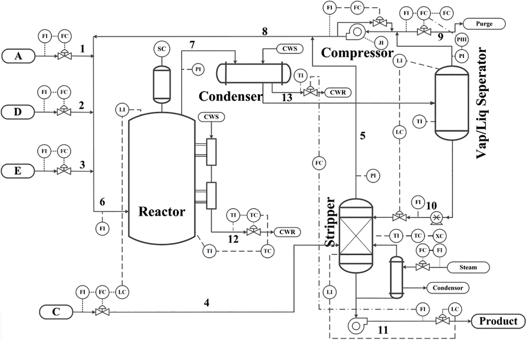
Figure 1: The control structure and flow diagram of TE process

The TE process contains four gaseous raw materials (A, C, D and E), two liquid products (G and H), and by-products (F) and inert gas (B). The irreversible, exothermic chemical reaction in TE process is as follows:

A(g)+C(g)+D(g)→G(l)A(g)+C(g)+E(g)→H(l)A(g)+D(g)→F(l)3D(g)→2F(g)(17)

The gas components (A, C, D and E) and the inert component (B) are fed into the reactor, thus forming the liquid products (G and H), where the reaction rate obeys the Arrhenius function of the reaction kinetics. Coming out of the reactor, the product steam is condensed to liquid and transferred to a liquid separator, from which a string of steam would be resent to the reactor through the compressor. Some recirculation shunt should be dismissed to avoid accumulating the by-products and inert components in the reaction. The condensed products from the separator (Steam 10) are sent to the stripper. Steam 4 is applied to remove the remaining reagents, in Steam 10, mixed with the recirculating steam from Steam 5. The products (G and H) are sent to the downstream process. Most of the by-products are evacuated as gas in the vapor-liquid separator. According to the different component mass ratios of G and H in the product, the TE process supports 7 operation modes/working conditions. The simulation platform can set 21 fault modes, e.g., the fault modes of step type, random change type, slow drift type, valve sticky type, valve stuck type and unknown types.

4.2 Experiment Setup

The TE process supports a variety of operation modes and a total of 28 prescribed fault types are given in detail. The simulated multi-mode data can be obtained from the TE process. A number of typical fault conditions in TE simulation dataset are selected, i.e., the TE process operation data without fault, and fault status #4, #10, #13, #16, #18 and #28. Then, the implementation process of the algorithm is described. We continuously extract a group pf time-series samples in different conditions (including different conditions with 6 faults and the normal condition). As shown in Table 1, two different operation modes are set up in this experiment.

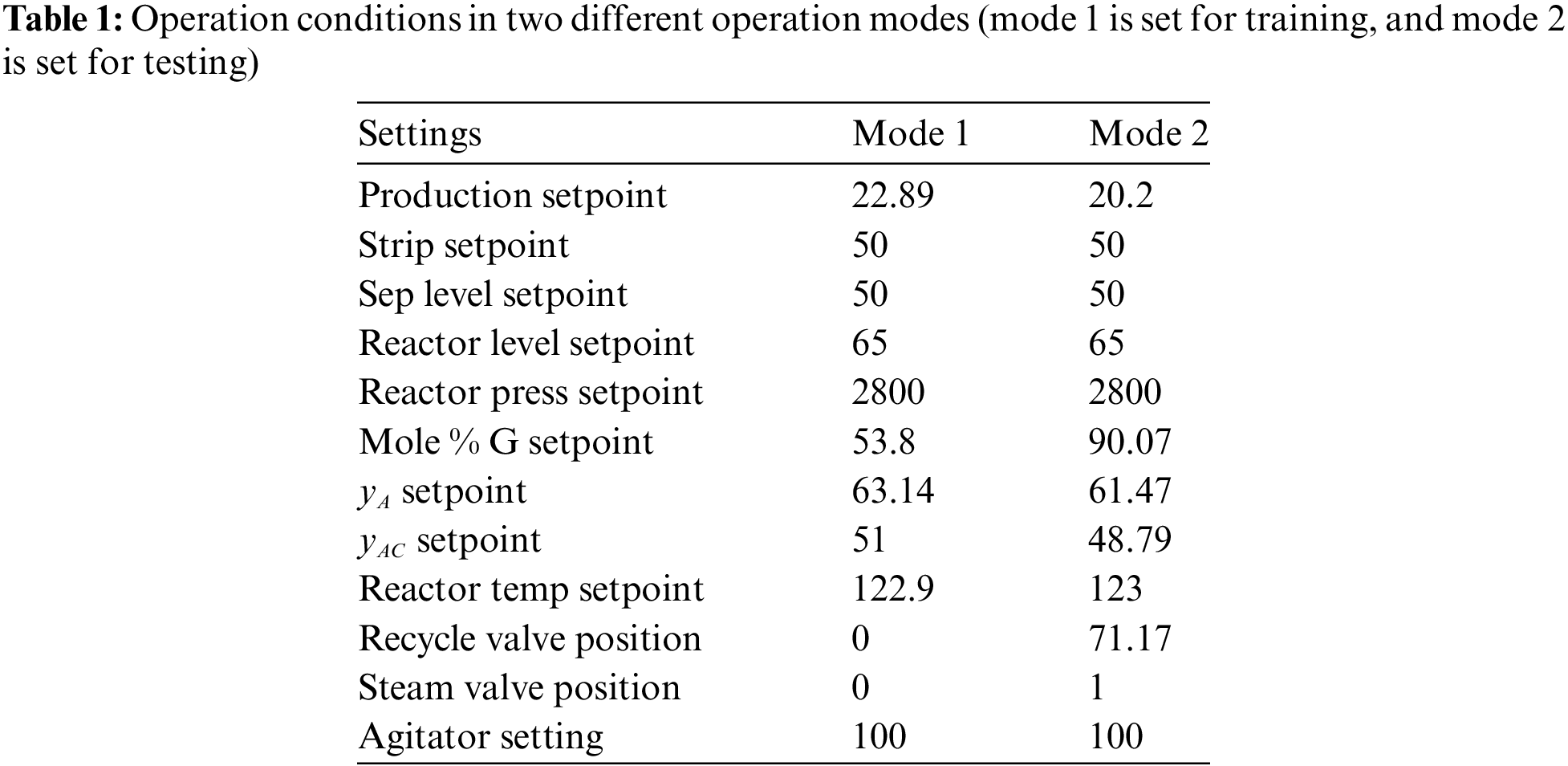
The training dataset contains the samples obtained in mode 1, in which the data in normal condition and in fault condition is 2400, respectively. Meanwhile the testing dataset contains samples obtained in mode 2, in which the data in normal condition and in fault condition is 200, respectively. The data generated in mode 1 is used to train the binary fault classification model, and the data generated in mode 2 is used to verify the TE process fault classification (i.e., classification accuracy). Since the training and testing datasets are obtained in different operation modes in TE process, it can be considered that the probability distribution of input samples in training datasets is different from that of the testing dataset. There exists the covariate shift phenomenon between the training dataset in operation mode 1 and the testing dataset in operation mode 2. To reduce the amount of data and increase the efficiency of the method, it is necessary to select some variables from all process variables, which have strong correlations with the fault variables. We introduce the mutual information for such a task. The MI is equivalent to dimensionality-reduction operation on the original data.

In the experiment, the MI-based variable selection works as follows: 1) re-arrange the variables in the training and testing dataset in the order of MI value; 2) choose 25 variables with largest MI value in the training and testing dataset, respectively; 3) observe the selected 25 variables, and select all the common variables among them; 4) calculate the MI value between the selected common variables, respectively, and remove these variables with low MI value (there is weak correlation or negative correlation, this operation is to prevent the occurrence of negative transfer); 5) delete other variables, the remaining variables are exactly the process variables we need, and these variables selected can be used to train the model of fault classification.

The MI-based pre-processing can not only reduce the computational workload, but also make the selected data more effective. On the other hand, in addition to data redundancy, not all the data are valid for fault classification and fault detection model. Some data have stronger correlation with the fault, and that the correlation between process variable and fault variable is not always the same. Besides, there is some data that cannot indicate whether there exist some faults in the process system, and the data is invalid for fault detection. Therefore, with the MI-based feature selection, we can extract more useful information for fault classification model and form the reorganized input dataset for training process. In this way, the data pre-processing can greatly eliminate the invalid samples and variables, and retain the most relevant variables for fault detection and classification.

The training and testing dataset processed by MI feature selection is input to IWLSPC for fault detection and classification. Specifically, we perform the testing with binary fault classification and multiple fault classification. In addition, the IWLSPC is compared with other existing methods in detail.

5  Experimental Result

5.1 Comparison of Binary Fault Classification Performances under Covariate Shift

Firstly, we apply the proposed method to the binary fault detection and classification of TE process. In fact, if the binary fault situation refers to the two categories of having some specific faults or no fault, then binary fault classification is equivalent to the judgement of the process fault, i.e., exist or not exist. Therefore, to improve the comparability of different binary fault classification, we classify all the fault categories with the case without fault, that is, the designed algorithms should be able to distinguish whether there exist some faults or not in the TE process under covariate shift. The detailed performance comparison of binary fault classification is shown in Table 2. Taking no fault and specific fault as the two labels of binary fault classification, the results presented are the accuracy of fault classification with the testing dataset. In addition, the results marked as  ∗ in the table are the results of data-driven fault classification model trained by the validation dataset with particularly few samples (only 200 samples), the results are used to demonstrate the effectiveness of importance-weighted transfer learning under covariate shift.

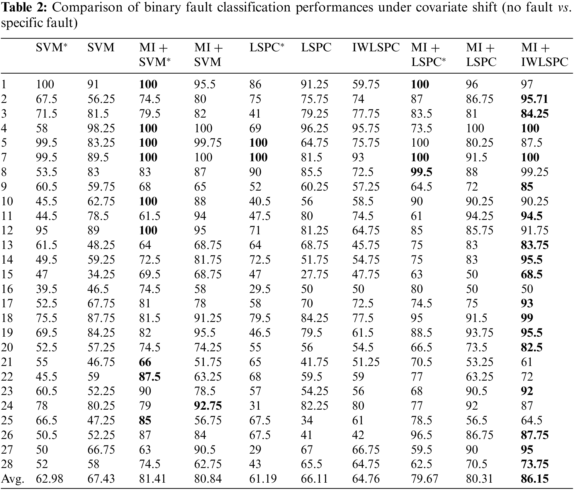
First, we sorted the correlation of the characteristics related to the fault according to their MI values, and then selected the most relevant process variables. The pre-processing can not only reduce the amount of data, but also significantly improve the effectiveness of the data training. We compared the performance of extracting feature variables with/without MI. As shown in Table 2, by introducing the MI to the extraction of variables, the IWLSPC can better detect whether a fault exists or not.

Because the training and testing datasets we use are obtained in different operation modes, the process dynamic characteristics and fault-related information contained in the training and testing datasets are inconsistent. Once the training process completes, the traditional machine learning based classifications cannot adapt to the change of operation modes in the testing dataset according to the sample distribution. The importance weighting used in this study considers the probability distribution of the test input samples during the training process, and it carries out the weighted re-organization of the training input samples based on the importance weights, which can improve the accuracy of fault classification on the testing dataset. As shown in Table 2, for most types of faults, the performance of the MI-based IWLSPC is better than that of the traditional LSPC, and the total average performance of 28 fault types is also better than the MI-based LSPC. The result shows that the IWLSPC can better detect whether there exists a fault under covariate shift. It achieves superior performance to detect whether there exist some specific faults or there do not exist faults for the current state.

Furthermore, we compared the effectiveness of commonly used machine learning based classification algorithms and applied them to the binary fault classification for the TE process. As shown in Table 2, we can see that in most cases, the IWLSPC achieves excellent fault classification performance. Although SVM has some advantages in some cases, IWLSPC achieves better fault classification performances in most of the fault types. However, the reliability of MI + IWLSPC can be guaranteed, which is exactly why MI-based IWLSPC outperforms for the total average fault classification accuracy. It is proven that LSPC and IWLSPC can not only be used to binary fault classification, but also can be applied to classify multiple faults simultaneously.

In order to demonstrate the effectiveness of importance-weighted transfer learning under covariate shift. We have also conducted experiments with extremely small samples, in which we directly train the fault classification model on the small dataset. Specifically, we trained the afore-mentioned fault classification models on the validation set with only 200 samples. This kind of small sample training is very practical for nonlinear multi-mode industrial processes, because some of the actual industrial processes usually do not have sufficient historical data under working conditions. The results marked with * in Table 2 show that the performance of directly training on the validation dataset is poor, because there is not sufficient data for the training process. However, with the importance-weighted transfer learning method, the data-driven fault classification model achieves satisfactory performance even on a small sample verification dataset where the covariate shift exists. It confirms the effectiveness of the importance-weighted transfer learning method.

5.2 Comparison of Multi-Fault Classification Performance with Other Methods

The probabilistic-based classification method for industrial process fault classification works well. In this study, we compared the effectiveness of the BP neural network, traditional LSPC and IWLSPC that is suitable for dealing with covariate shift. It is noted that we used MI to extract feature variables in both methods, thus mainly focusing on the difference among BP neural network, LSPC and IWLSPC, i.e., the effectiveness of the importance-weighted method. The detailed comparison is shown in Table 3.

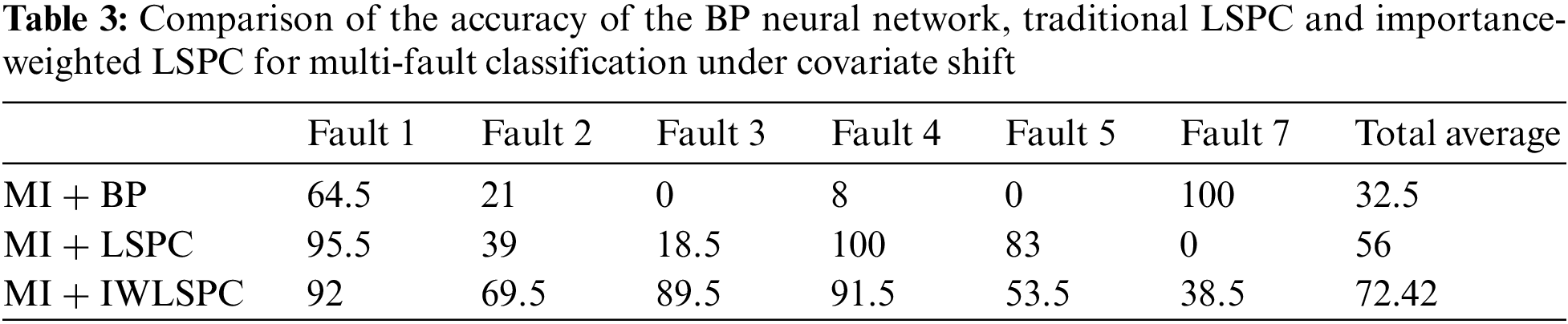
In Table 3, the effectiveness of the IWLSPC algorithm for multi-fault classification of the TE process under covariate shift is detailed. According to Table 3, we can conclude that the IWLSPC achieves better performance for the simultaneous classification for multiple faults in the TE process. Especially in some cases, the accuracy of the IWLSPC is much higher than that of the traditional LSPC, which confirms the effectiveness of IWLSPC. In addition, it is noted that although the BP neural network is extremely effective in the classification of certain types of faults, the classification performance of this method under different conditions has serious fluctuations, resulting in a very poor average performance.

6  Conclusion

In this paper, the importance-weighted sampling is introduced to address the problem of inconsistent data distribution in training and testing dataset, and it is designed for the fault classification in the multi-mode industrial process, especially for the nonlinear multi-mode industrial process. In the case of covariate shift, it can smoothly adapt to the multi-mode dataset and achieve good performances for fault classification. Besides, we have also confirmed that the introduction of MI for feature selection significantly improves the performance of the fault classifier. This is because the MI can select specific features closely related to these faults. It not only reduces the computational workload, but also gets rid of those variables that are irrelevant to fault classification. In order to address the limitations of the present method, in the future, we will take the ratio of posterior density into consideration, which is calculated in line with the importance-weight estimation and can theoretically break through the assumption that the posterior probability does not change between the training and testing phases. In order to improve the efficiency of feature selection, we will focus on those methods, which can effectively extract feature combinations to improve the performance of negative migration-enhanced classifiers. Besides, in the future, we will try other tools to further improve the efficiency of the optimization.

Acknowledgement: None.

Funding Statement: The authors received no funding for this study.

Author Contributions: Conceptualization, Methodology, Software, Data Curation, Writing—Original Draft Preparation: Yi Pan; Investigation, Validation, Writing—Reviewing: Lei Xie; Supervision: Hongye Su. All authors reviewed the results and approved the final version of the manuscript.

Availability of Data and Materials: The data that support the findings of this study are available from the corresponding author, Lei Xie, upon reasonable request.

Conflicts of Interest: The authors declare that they have no conflicts of interest to report regarding the present study.

References

1. Z. Ge and J. Chen, “Plant-wide industrial process monitoring: A distributed modeling framework,” IEEE Trans. Ind. Inform., vol. 12, no. 1, pp. 310–321, 2016. doi: 10.1109/TII.2015.2509247. [Google Scholar] [CrossRef]

2. L. Yao and Z. Ge, “Industrial big data modeling and monitoring framework for plant-wide processes,” IEEE Trans. Ind. Inf., vol. 17, no. 9, pp. 6399–6408, 2021. doi: 10.1109/TII.2020.3010562. [Google Scholar] [CrossRef]

3. Z. Ge, “Review on data-driven modeling and monitoring for plant-wide industrial processes,” Chemometr. Intell. Lab. Syst., vol. 171, no. 2, pp. 16–25, 2017. doi: 10.1016/j.chemolab.2017.09.021. [Google Scholar] [CrossRef]

4. R. H. Raveendran and B. Huang, “Process monitoring using a generalized probabilistic linear latent variable model,” Automatica, vol. 96, no. 7, pp. 73–83, 2018. doi: 10.1016/j.automatica.2018.06.029. [Google Scholar] [CrossRef]

5. Q. Jiang, X. Yan, and B. Huang, “Review and perspectives of data-driven distributed monitoring for industrial plant-wide processes,” Ind. Eng. Chem. Res., vol. 58, no. 29, pp. 12899–12912, 2019. doi: 10.1021/acs.iecr.9b02391. [Google Scholar] [CrossRef]

6. Z. Yang and Z. Ge, “Monitoring and prediction of big process data with deep latent variable models and parallel computing,” J. Process Control, vol. 92, no. 11, pp. 19–34, 2020. doi: 10.1016/j.jprocont.2020.05.010. [Google Scholar] [CrossRef]

7. L. Luo, L. Xie, H. Su, and F. Mao, “A probabilistic model with spike-and-slab regularization for inferential fault detection and isolation of industrial processes,” J. Taiwan Inst. Chem. Eng., vol. 123, no. 1, pp. 68–78, 2021. doi: 10.1016/j.jtice.2021.05.047. [Google Scholar] [CrossRef]

8. K. Wang, J. Chen, Z. Song, Y. Wang, and C. Yang, “Deep neural network-embedded stochastic nonlinear state-space models and their applications to process monitoring,” IEEE Trans. Neural Netw. Learn. Syst., vol. 33, no. 12, pp. 1–13, 2021. [Google Scholar]

9. S. Yin, X. Steven, X. Xie, and H. Luo, “A review on basic data-driven approaches for industrial process monitoring,” IEEE Trans. Ind. Electron., vol. 61, no. 11, pp. 6418–6428, 2014. doi: 10.1109/TIE.2014.2301773. [Google Scholar] [CrossRef]

10. L. Luo, L. Xie, and H. Su, “Deep learning with tensor factorization layers for sequential fault diagnosis and industrial process monitoring,” IEEE Access, vol. 8, pp. 105494–105506, 2020. doi: 10.1109/ACCESS.2020.3000004. [Google Scholar] [CrossRef]

11. X. Deng, N. Zhong, and L. Wang, “Nonlinear multimode industrial process fault detection using modified kernel principal component analysis,” IEEE Access, vol. 5, pp. 23121–23132, 2017. doi: 10.1109/ACCESS.2017.2764518. [Google Scholar] [CrossRef]

12. M. Sugiyama and M. Kawanabe, Machine Learning in Non-Stationary Environments: Introduction to Covariate Shift Adaptation. The MIT Press, 2012. [Google Scholar]

13. H. J. Song and S. B. Park, “An adapted surrogate kernel for classification under covariate shift,” Appl. Soft Comput., vol. 69, no. 3, pp. 435–442, 2018. doi: 10.1016/j.asoc.2018.04.060. [Google Scholar] [CrossRef]

14. M. T. Amin, F. Khan, S. Imtiaz, and S. Ahmed, “Robust process monitoring methodology for detection and diagnosis of unobservable faults,” Ind. Eng. Chem. Res., vol. 58, no. 41, pp. 19149–19165, 2019. doi: 10.1021/acs.iecr.9b03406. [Google Scholar] [CrossRef]

15. L. Qi et al., “A correlation graph based approach for personalized and compatible web APIs recommendation in mobile APP development,” IEEE Trans. Knowl. Data Eng., vol. 35, no. 6, pp. 5444–5457, 2022. doi: 10.1109/TKDE.2022.3168611. [Google Scholar] [CrossRef]

16. Y. H. Yang et al., “ASTREAM: Data-stream-driven scalable anomaly detection with accuracy guarantee in IIoT environment,” IEEE Trans. Netw. Sci. Eng., vol. 10, no. 5, pp. 3007–3016, 2022. doi: 10.1109/TNSE.2022.3157730. [Google Scholar] [CrossRef]

17. F. Wang et al., “Privacy-aware traffic flow prediction based on multi-party sensor data with zero trust in smart city,” ACM Trans. Internet Technol., vol. 23, no. 3, pp. 1–19, 2022. [Google Scholar]

18. L. Y. Qi, Y. H. Yang, X. K. Zhou, W. Rafique, and J. H. Ma, “Fast anomaly identification based on multi-aspect data streams for intelligent intrusion detection toward secure Industry 4.0,” IEEE Trans. Ind. Inform., vol. 18, no. 9, pp. 6503–6511, 2022. doi: 10.1109/TII.2021.3139363. [Google Scholar] [CrossRef]

19. H. Q. Wu et al., “Popularity-aware and diverse web APIs recommendation based on correlation graph,” IEEE Trans. Comput. Soc. Syst., vol. 10, no. 2, pp. 771–782, 2022. doi: 10.1109/TCSS.2022.3168595. [Google Scholar] [CrossRef]

20. S. J. Pan and Q. Yang, “A survey on transfer learning,” IEEE Trans. Knowl. Data Eng., vol. 22, no. 10, pp. 1345–1359, 2010. doi: 10.1109/TKDE.2009.191. [Google Scholar] [CrossRef]

21. H. Han, Z. Liu, H. Liu, and J. Qiao, “Knowledge-data-driven model predictive control for a class of nonlinear systems,” IEEE Trans. Syst. Man Cybernet.: Syst., vol. 51, no. 7, pp. 4492–4504, 2021. [Google Scholar]

22. C. Li et al., “Fabric defect detection in textile manufacturing: A survey of the state of the art,” Secur. Commun. Netw., vol. 2021, no. 1, pp. 1–13, 2021. doi: 10.1155/2024/5034640. [Google Scholar] [CrossRef]

23. S. Chen and X. Yang, “Tailoring density ratio weight for covariate shift adaptation,” Neurocomputing, vol. 333, no. 2, pp. 135–144, 2019. doi: 10.1016/j.neucom.2018.11.082. [Google Scholar] [CrossRef]

24. H. Shimodaira, “Improving predictive inference under covariate shift by weighting the log-likelihood function,” J. Stat. Plan. Infer., vol. 90, no. 2, pp. 227–244, 2000. doi: 10.1016/S0378-3758(00)00115-4. [Google Scholar] [CrossRef]

25. M. Sugiyama, “Learning under non-stationarity: Covariate shift adaptation by importance weighting,” in Handbook of Computational Statistics: Concepts and Methods, Berlin, Heidelberg: Springer, 2012, pp. 927–952. [Google Scholar]

26. Y. Tsuboi, H. Kashima, S. Hido, S. Bickel, and M. Sugiyama, “Direct density ratio estimation for large-scale covariate shift adaptation,” Inf. Med. Technol., vol. 4, no. 2, pp. 529–546, 2009. doi: 10.2197/ipsjjip.17.138. [Google Scholar] [CrossRef]

27. F. Lu et al., “Zhu etal, HFENet: A lightweight hand-crafted feature enhanced CNN for ceramic tile surface defect detection,” Int. J. Intell. Syst., vol. 37, no. 12, pp. 10670–10693, 2022. doi: 10.1002/int.22935. [Google Scholar] [CrossRef]

28. F. Lu, R. Niu, Z. Zhang, L. Guo, and J. Chen, “A generative adversarial network-based fault detection approach for photovoltaic panel,” Appl. Sci., vol. 12, no. 4, pp. 1789, 2022. doi: 10.3390/app12041789. [Google Scholar] [CrossRef]

29. Z. Ge and Z. Song, “Process monitoring based on independent component analysis−principal component analysis (ICA−PCA) and similarity factors,” Ind. Eng. Chem. Res., vol. 46, no. 7, pp. 2054–2063, 2007. doi: 10.1021/ie061083g. [Google Scholar] [CrossRef]

30. L. Xie, X. Lin, and J. Zeng, “Shrinking principal component analysis for enhanced process monitoring and fault isolation,” Ind. Eng. Chem. Res., vol. 52, no. 49, pp. 17475–17486, 2013. doi: 10.1021/ie401030t. [Google Scholar] [CrossRef]

31. Q. Wen, Z. Ge, and Z. Song, “Multimode dynamic process monitoring based on mixture canonical variate analysis model,” Ind. Eng. Chem. Res., vol. 54, no. 5, pp. 1605–1614, 2015. doi: 10.1021/ie503324g. [Google Scholar] [CrossRef]