Transformation of MRI Images to Three-Level Color Spaces for Brain Tumor Classification Using Deep-Net

1  Introduction

The human brain is like the control center for the human body. It takes information from our senses, processes it, and tells human muscles what to do. Abnormal growth of brain cells called brain tumors, can be a serious problem. Additionally, the World Health Organization (WHO) has categorized brain tumors (BTs) into four groups (Grades I–IV) based on how severe they are [1]. In the field of medical science, there has been a lot of development in several imaging techniques to aid in the diagnosis of diseases. These include X-rays, ultrasound, PET scans, CT scans, MRS, SPECT scans, and MRI [2]. These imaging technologies provide valuable insights for doctors to examine different parts of the human body, ensuring the diagnosis and treatment of various diseases. Among these, MRI stands out as the preferred and most valuable method because it shows images with high resolution and provides accurate details about the structure of the body. It is especially effective in capturing many types of brain tumors like Glioma, Pituitary tumors, and Meningioma [3]. Fig. 1 shows the brain tumor types. In fact, MRI is widely regarded as one of the most reliable and widely used tools for classifying brain tumors. Grade III and Grade IV BTs are especially fast-growing tumors and can spread to other parts of the body, harming different healthy cells. Detecting and identifying BTs early is crucial because it helps doctors to plan the right treatment, using tools like MRI and other images [4].

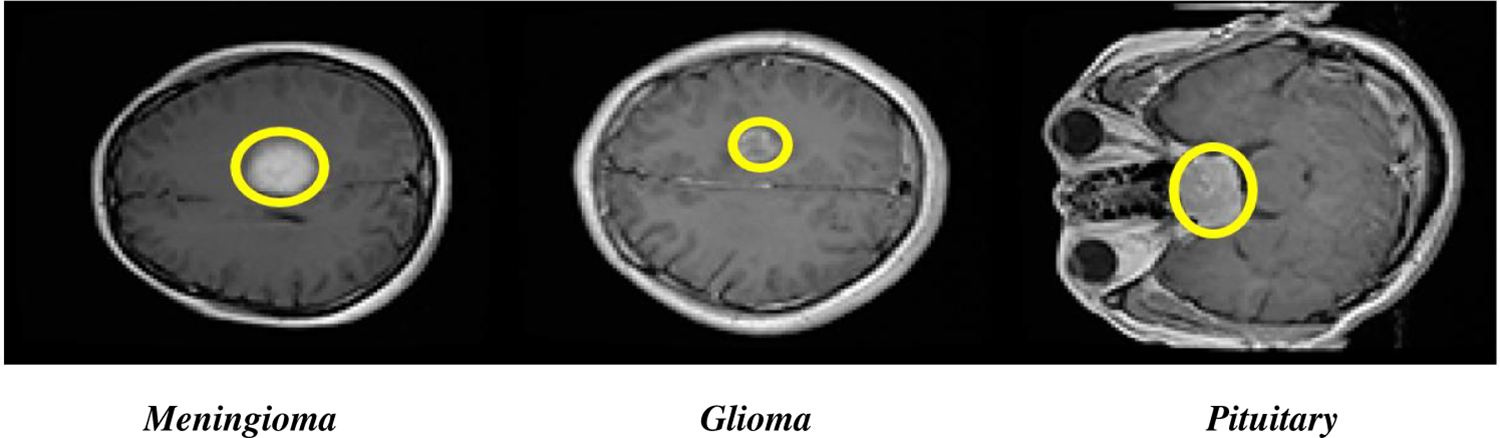
Figure 1: Axial view of Glioma, Pituitary brain tumors, and Meningioma types

There are three types of primary brain tumors: Glioma, Pituitary tumors, and Meningioma. Pituitary tumors are generally non-cancerous that grow in pituitary glands, which produce vital hormones in the body [5]. Gliomas develop from specific brain cells called glial cells [6]. Meningioma tumors usually grow on the protective and outer membrane that covers the spinal cord and brain [7]. Identifying the difference between normal brain tissue and abnormal tissue is vital when looking for BTs. Due to differences in size, shape, and location, detecting BTs can be challenging and still an ongoing problem to be addressed. The field of medical images processing plays an important role for BT analysis, including tasks like classification, segmentation, and detection [8,9]. The accurate classification of brain tumor is necessary to diagnose the tumor type timely if it exists. Modern diagnosis systems aided by computer in biomedical image processing to help radiologists in guiding patients and improve BT classification [10,11]. For brain tumor categorization, the use of advanced and pre-trained CNN models has made great progress, allowing researchers to make speedy and accurate decisions. Due to the complexity of data, categorizing brain images with high accuracy remains a difficult challenge. Using publicly available datasets, this study aims to develop a completely automatic CNN model that performs color transformation and selects optimized features for identifying brain tumors into different categories.

The motivation for this research to study hidden brain tumors in image datasets stems from this important goal and to enhance the early detection and diagnosis of these tumors. Accurate identification of brain tumors is a challenging due to their subtle and complex pattern. By focusing on camouflaged tumors within image datasets, researchers are dedicated to develop advanced image processing and machine learning algorithms, the aim is to enhance the detection and classification of these hidden tumors with high precision and efficiency. Early detection can significantly improve patient outcomes by assisting timely medical interventions and treatment strategies, eventually lead to improve prognosis and an enhanced quality of life for individuals dealing with this condition. Color transformation plays an important role by enhancing the visual representation of grayscale images, assisting in the accurate interpretation and analysis of tumor patterns and structures. Our proposed methodology outperforms in the existing deep learning approaches in terms of classification accuracy, even with reduce amount of training data, as described in the confusion matrix.

The proposed approach for classifying BT consists of three steps: Improving contrast, transforming images into color spaces, fusing multiple feature fusion, and feature selection for final classification. The following are the important contributions of this approach:

•   A novel technique known as MRI image modification is introduced to improve the contrast in MRI brain tumor pictures, aiming to improve the internal contrast of the robust feature selection for brain tumor camouflage.

•   The ResNet50 model is applied for feature extraction, focusing on the weighted features of the first convolutional layer through three distinct color transformations. These features are joined using a sequential canonical correlation-based technique.

•   The Marine Predator Algorithm (MPA) is used to select features and employ diverse machine learning based classifiers with different learning rate and cross validation techniques.

2  Literature Review

Many techniques have been introduced over time to classify and segmentation of BT data. While more modern methods have made use of deep learning models [12], some of these techniques still rely on conventional machine learning. We focus on BT classification research in this section.

There are several methods that have been proposed, incorporating transfer learning on custom dataset, deep CNN features extraction and classification, and deep ensemble methods to achieve better accuracy. In [13], authors introduced a neural network and segmentation base framework that automatically detects tumors in brain MRI images. To evaluate feature extraction from an MRI brain image, the methodology extended PCA and different classifiers are used for feature classification. The average rate of recognition is 88.2%, and a peak rate of 96.7%. Tazin et al. [14] defined a model aimed at increasing accuracy by transfer learning techniques. They applied three different techniques that used pre-trained CNN models and obtained accuracy rates of 88.22% using VGG19, 91% using Inception V3, and 92% using Mobile Net V2, respectively. In comparison to the other models, the authors found that MobilnetV2 is far more useful. In [15], Abd-Ellah et al. presented a PDCNN framework to identify and categorizing gliomas in MRI images. Dataset (The braTS-2017) employed to evaluate the proposed PDCNNs. The study uses 1200 photographs in the PDCNN training phase, 150 images in the PDCNN for validity purpose, and 450 images are in the PDCNN test phase. This framework produced 97.44% accuracy, 97.0% sensitivity, and 98.0% specificity. Afshar et al. [16] proposed using capsule networks to serve as a CNN topology with a precision of 90.89%, the proposed technique employs the Figshare dataset to focus on the major location of tumors and their relationships to nearby tissues. In [17], Nazir et al. proposed a model using the ANN technique. Groups of two malignancies have been targeted in their proposed research: Beginning stage tumors and malignant tumors. In the first stage, images are preprocessed with filters then the average color moment approach is used to extract features. After characteristic mappings to the ANN classification accuracy is 91.8%. In [18], Luyan et al. developed a system that is capable of extracting outcomes from the connectome of a complex human brain by expanded network analysis strategies. As a result, they used a multistage feature selection technique to select those features that lessens the feature redundancy. Hence, they used a support vector machine (SVM) to generalize the outcomes of HGG, the result was not respectable and moral. Finally, their approach attained an accuracy of 75%. Sawant et al. [19] devised a strategy that highlights the tensor flow procedure to detect brain tumors using MRI. 5-layer CNN model implemented using tensor flow. A total of 1800 MRIs were used on the dataset, with 900 of them being tumors and the other 900 being non-tumorous. Among 35 epochs, tanning accuracy was 99% and validation accuracy was 98.6%.

Researchers used many model based and features selection-based methods. In [20], Soesanti et al. suggested a model using the statistical histogram equalization technique, that applies a transformation to each and every pixel by the calculation of multiple statistical parameters like variance, entropy, etc. This model is used to define low and high-level images of cervical glioma. The idea is to achieve an accuracy level of 83.6%, a sensitivity rate of 80.88%, and 86.84% of specificity. In [21], the authors used the features of a pre-trained model and employed a genetic algorithm for feature selection. This novel method produced outstanding results, achieving an astounding 95% accuracy on two challenging datasets, BRATS2018 and BRATS2019. Attique et al. [22] also used a multimodal approach to classify BT images where, for features extraction used VGG16 and VGG19. In addition, the authors achieved 95.2% results on the BraTs2018 dataset. In a similar work proposed in [23], the author extracted deep features for the segmenting, localization, and classifying of brain tumors, achieving the best accuracy of 95.71% on the selected brain tumor dataset. Francisco et al. [24] introduced deep CNN based BT segmentation and classification on the T1-CE MRI images dataset for multi-class type tumor classification and the authors got good accuracy on the selected dataset. In [25], Çinar et al. developed a hybrid strategy for brain tumor identification in which the tumor was identified from MRI using deep learning algorithms. CNN model was employed to predict eight additional layers and remove the last five layers from ResNet50. As a result, their created model outperformed than other deep learning models by 97.2%. In [26], Anil et al. proposed a technique, which includes a network of classification algorithms that divides the MRI images into two categories: Those with tumors and those without. The classification system was retrained to identify brain tumors using the technique of transfer learning. According to the results, VGG19 was really effective, accuracy of percentage of 95.78%.

3  Proposed Methodology

In this section, a novel and comprehensive model is presented for MRI image transformation into vibrant color. A pre-trained CNN model ResNet50 is employed to extract deep features from grayscale MRI images, which are then fused, selected, and classified. The overall proposed model of MRI image transformation is presented in Fig. 2.

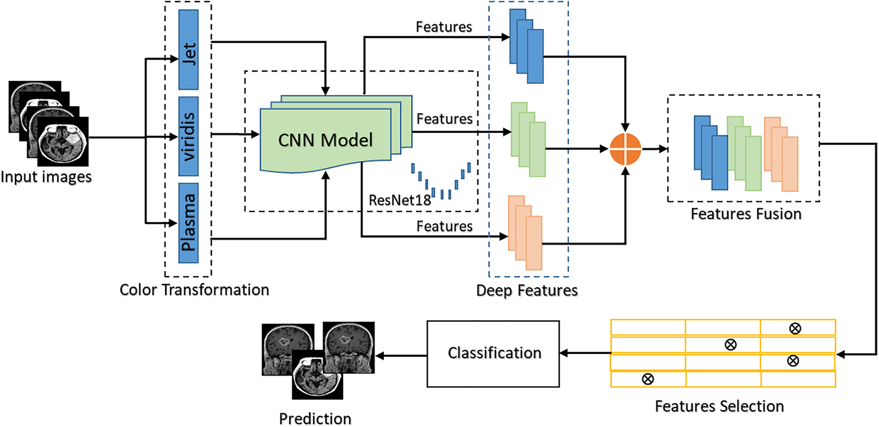
Figure 2: Proposed system diagram

The models specify brain tumor classification and support on unique imaging features may bound its applicability to varied disorders with diverse indicators as well as can to detect camouflaged brain tumors. Acquiring diverse and illustrative training data for numerous conditions is crucial but may be challenging, possibly affecting the model’s performance. The resource-intensive nature of profound neural networks, probable issues with toughness and transfer learning, and obedience to regulatory standards further underline the complications involved in ranging the model beyond its original focus on brain tumors. Addressing these challenges requires a thoughtful approach, including proven authentication, association with domain professionals, and reflection of monitoring compliance to confirm the model’s responsibility and operating application across various medical imaging situations.

This proposed model has been carefully tested in three main steps. First, grayscale images are converted into color images after that color MRI images are transformed into: Plasma, Viridis, and Jet. To extract strong visual features from each category a pre-trained CNN model is used. In the second step, these features are then fused together in a single feature vector which selectively holds the most relevant information. Feature selection is applied to classify MRI images. This procedure results in successful MRI image categorization, resulting in findings that are both informative and visually appealing. The following sections provide a detailed description of various modules.

3.1 Preprocessing

In the preprocessing step, grayscale MRI images are resized to enhance further colorization while improving the model’s reliability and adaptability. To reduce the resolution of the MRI images, the most common approach is to scale them to a rectangular format with appropriate dimensions. In this proposed work 224 × 224 size input images are used to train our model. After resizing the image, the next step is to remove the noise.

Noise removal in brain MRI images is typically advantageous as it enhances the picture quality, making the images easier to read and assisting inaccurate diagnosis. In this proposed work Gaussian filter is used for noise reduction. The Gaussian filtration is defined as follows:

G(ao,i0)=12πσ2−(ao2+i02)2σ2(1)

where G(ao,i0) is the Gaussian function at coordinates (x, y) and σ represents the value of standard deviation in Gaussian distribution.

After removing the noise from MRI images normalization is the next and an important step before color transformation. The next step is normalization MRI images, as grayscale images are going to be converted into colorized images. The procedure starts with selecting grayscale MRI images and learning about their pixel value range, which typically ranges from 0 to 255. A linear scaling process is used to normalize these grayscale images, which typically rescales the pixel to [0, 1] or [−1, 1]. This rescaling creates a strong base for further color transformation. Differences in pixel value scales do not affect color transformation and generate visually appealing colorized MRI images. To calculate the range from [0, 1] normalization is applied as:

Inormalize=x−xminxmax−xmin(2)

To calculate the range from [−1, 1] normalization is applied as:

Inormalize=2∗(x−xmin)(xmax−xmin)∗−1(3)

where Inormalize is the new value, xmin is the minimum pixel value and xmax maximum pixel value. After normalization, all grey scale pixels are normalized within a specified range which is more suitable for color transformation.

3.2 Color Transformation

Color transformation is the process of transforming grayscale images into visually appealing color images. In this proposed work colorization process is a fundamental step. In the first step, normalized greyscale images are transformed into colored images to enhance visual understanding and diagnostic accuracy. The MRI image of the human brain is extremely complex, with several structures and types of tissue that can be difficult to detect in grayscale. Different anatomical spots or pathologies and abnormalities become more visibly apparent when color is introduced. In the medical field, the majority of grayscale images require colorization to help the doctor for detailed understanding. We convert Inormalize MRI images into colored images by this equation:

Icolor=Concat(Inormalized+Inormalized+Inormalized)(4)

In the second step, colored MRI images are then transformed into three color spaces: Plasma, Viridis, and Jet. These color spaces highlight different features of the MRI images and enhance visual aspects of the image which can fulfill the diagnostic and analytical needs. Plasma, Viridis, and Jet all highlight different features, such as structural features, and tissue contrast. The Plasma color spaces are made up of gradients, and their transformation can be expressed by this equation:

Iplasma=(0.1717∗G)+(0.757∗B)−(0.1882∗G∗B)(5)

In this equation, to find the color space of plasma Green (G) and Blue (B) components are used in this calculation. The coefficients 0.1717, 0.757, and 0.1882 determine the contribution of G and B to Plasma color space. To find the Virdis, the equation which is used as follows:

Iviridis=(0.1696∗G)−(0.3544∗R)+(0.5679∗B)(6)

In this equation, the coefficients 0.1696, 0.3544, and 0.5679 are used to determine Viridis color spaces and are also calculated by Red (R) and Blue (B) components. For Jet color space, the equation is used as follows:

Ijet=(0.3016∗R)+(0.1979∗G)−(0.4287∗B)(7)

The contributions of R, G, and B to find the jet color space are determined by the coefficients 0.3016, 0.1979, and 0.4287. After the transformation of colored images into Plasma, Viridis, and Jet as depicted in Fig. 3, the next step is to extract features from these transformed images.

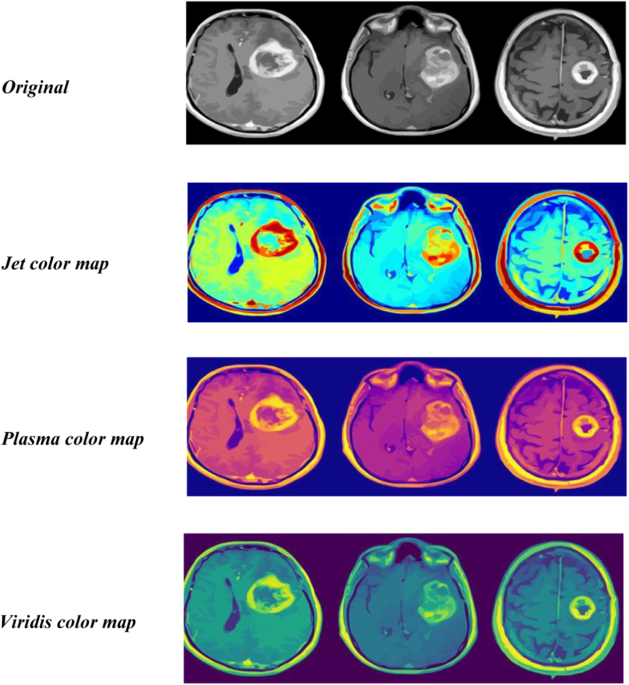
Figure 3: Transformation Plasma, Viridis, and Jet of sample images

The primary objective of color transformation is to identify the essential features for achieving precise classification outcomes. In addition, the visual illustration of the data can influence the capability to distinguish among different configurations or tissues in the MRI. This differentiation is vital for precise classification. Certain color maps may high spot image artifacts contrarily. Finding and understanding artifacts is essential for preprocessing steps and improving the strength of classification models. Though the color map choice is vital for visualization and understanding, it is just one feature of the overall heterogeneity data analysis. Moreover, the accuracy of classification is usually influenced by the features extracted from the data, the choice of the classification algorithm, and the quality of the training data, between other features. Consequently, the development in classification accuracy, if any, would expected to be a result of a more contemporary analysis and interpretation simplified by the use of suitable color maps. It might see which one provides the most efficient illustration for distinguishing related features in provided MRI data by testing with different color maps.

3.3 Transfer Learning

In computer vision transfer learning Tl is commonly represented by utilizing pre-trained models. Models that have been trained before can be employed due to the high computational expense of training such models from scratch. In transfer learning, define feature vector fv={vplasma,vviridis,vjet} and probability distribution as X={fv,P(fv)}. In which ground truth G={j1,j2,…,jn} and objective function O={G,L(x)}, whereas L(x) is an unknown label class. P(j|x) is a probabilistic function. Tl and lrate represent transfer learning and learning rate, respectively. (I(Tf)) represents the targeted function, while Tf represents the targeted output. The main objective of transfer learning in this proposed study is to improve the learning rate to predict the targeted object by using the recognition function (L(x)) based on the training learned from Tl and Tf where Tl≠Tf and lrate≠Tf.

3.3.1 Feature Extraction and Fusion Using Pre-Trained ResNet50

For deep feature extraction, a pre-trained CNN model ResNet50 is employed because it is an advanced feature extractor, completing a sequence of computations, this model generates in detailed feature maps. This model selection is for its great resilience and effectiveness in biological data analysis applications. The goal of using this model is to analyze images of various sizes and obtain depth characteristics. To finish this procedure, we first extend the 32 × 32 image to 224 × 224 × 3. As input for pre-trained models, we transform Icolor into a three-color space Iplasma, Iviridis, Ijet. These color maps enable better visual representations of brain structures and give a multidimensional perspective of the MRI images, boosting the interpretability of the model to grasp subtleties.

This approach recognizes the diverse information provided by each color map category and uncovers unique visual information that is related to each category during it scanning process. Jet may highlight certain structures, Viridis could emphasizes many others, and Plasma may expose still another aspect, resulting in an array of feature vectors Fv. The training process on image is performed by using DCNN pre-trained models to get features via the FC7 layer. We use Global Average Pooling (GAP) to combine these maps and transform them into feature vectors for each category. The global average pool is referred to as Fplasma,FViridis, and Fjet, respectively.

The combination of features from three color spaces is used to conduct feature fusion. The fusion of these three is carried out as follows:

Fus=[FJetFViridisFPlasma](8)

As a result, the concatenation process increases feature diversity, allowing the classifier to perform better. Subsequently, these characteristics are fused and concatenated to get deep features from this proposed model.

3.4 Feature Selection

Feature selection is the most important phase in the study and it is critical for improving the model’s efficiency and interpretability. A significant Fv is obtained after feature extraction from the three-color spaces (Jet, Viridis, and Plasma). After feature extraction, high dimensionalities may be encountered. This dimensionality reduction is done with care because it finds a balance between computing efficiency and the retention of important information inside the MRI images. Reducing the number of features reduces execution time while increasing performance. The outcome of feature selection is a single feature vector that provides data for subsequent classification tasks which improves the overall accuracy. The Marine Predator Algorithm (MPA) is used to select features; it is a nature-inspired algorithm.

The Marine Predator Algorithm (MPA) influences bio-inspired principles, pretending predatory crescendos of marine types. Over mathematical formulation, population initialization, and obliging hunting, MPA competently explores way out spaces for optimization difficulties. Predators dynamically adjust positions using movement and enclosing strategies, causative to solution convergence. Fine-tuning constraints, describing convergence criteria, and speaking algorithmic complexity make sure practical applicability. MPA’s achievement lied in its simulation of marine performances, offering an adaptive and effective optimization methodology with broad applications in varied domains, from engineering to artificial intelligence.

In MPA by combining exploration and exploitation methods, predators update their position. A simplified predator position update equation is:

pia=pia−1+Δpia(9)

In this equation, i is the initial position and a is the attempt pia−1 shows the previous position of the predator, Δpia shows the change in location as a result of hunting and foraging techniques. The next step is fitness evaluation using the objective function f(t), where t denotes the predator’s current position.

Fitness(pia)=f(pia)(10)

After fitness evaluation, the next step is to find the best-optimized solution. A basic formula for finding the best-optimized solution is:

pia+1=BestSelect(pia,pja,……..pna)(11)

where BestSelect is a feature selection process used to select the best-optimized features, then selected features are classified using some highly effective classification classifiers. These classifiers are super-smart, and we employ them to determine which group each colored image belongs to. We use performance metrics to evaluate how accurate our model is and to what extent it is good at detecting the appropriate tumors in colored MRI images. We can also calculate accuracy, precision, and recall ensuring our model’s correctness with different classifiers.

4  Result and Experimental Setup

To conduct experiments, this study utilized a dataset consisting of 7023 BT images collected from three different sources: Figshare [27], SARTAJ and Br35H described in [28] collected was downloaded from the Kaggle compiled by Masoud [29]. These images were categorized into four distinct classes, encompassing both normal brain images and three specific types of brain tumors, namely Glioma, Meningioma, and Pituitary tumors. Moreover, the proposed integrated brain tumor classification system was implemented using MATLAB 2022b on a computer with an Intel Core i7 processor, 16 GB of RAM, and an 8 GB graphics card. A series of different experiments are performed to evaluate the proposed model.

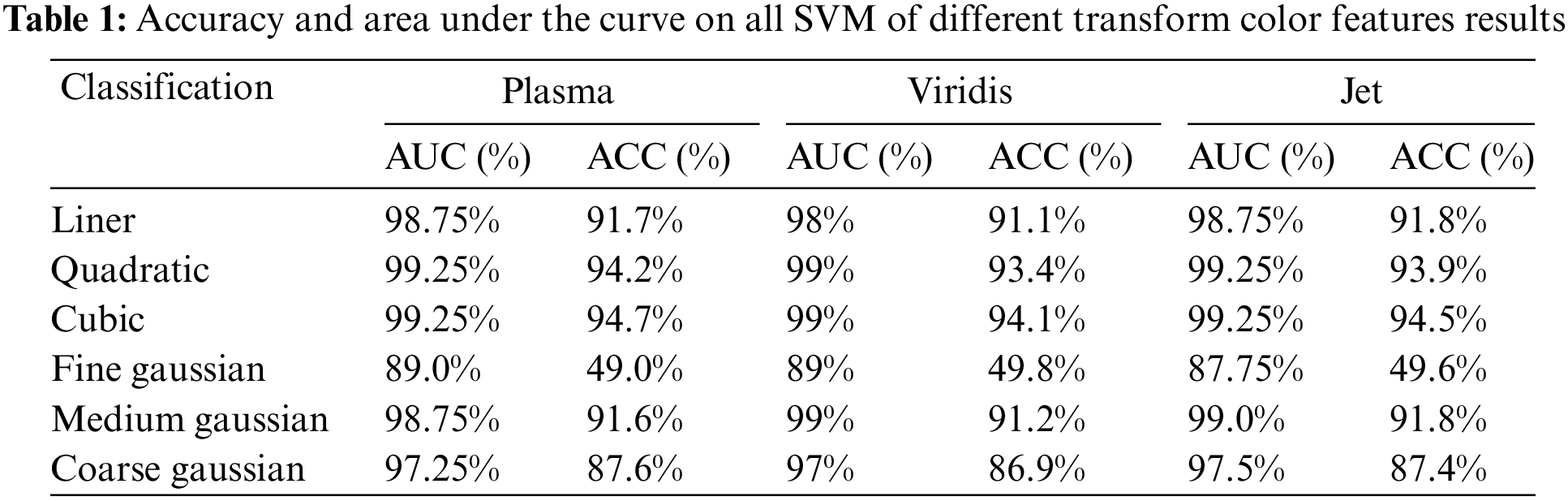
In the initial experiment as shown in Table 1, the primary objective was to evaluate the classification model’s accuracy in the context of brain tumor classification. For this experiment we utilize the ResNet50 architecture, a powerful and established deep learning model. The core focus of the experiment was to evaluate the model’s ability to accurately classify brain tumor images across various color transformations.

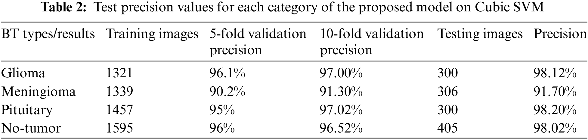
In this experiment as presented in Table 2 shows that, the test results for our model with four distinct classes as discussed above, notably achieved impressive precision rate for each category up to 98.12% for Glioma, 91.7% Meningioma, and so on. These precision scores provide insights into the accuracy of our classification for each class, ensuring robust performance and reliability in our model’s predictions.

In the next experiment as presented in Table 3, we harnessed the capabilities of well-established pre-trained models, including GoogleNet, ResNet18, and ResNet50, to extract discriminative features. Employing Support Vector Machines (SVM) for classification, we observed that Cubic SVM emerged as the top-performing classifier among the three models, GoogleNet, ResNet18, and ResNet50 and results are 95.5%, 95.2% and 98.4% achieved high accuracy, respectively. This approach demonstrated favorable results, underscoring the efficacy of utilizing Cubic SVM for accurate and effective classification. Cubic SVM performed well because functions as a non-linear classifier, enabling it to effectively represent intricate data relationships that might not be linearly distinguishable. Particularly in image classification, where decision boundaries can be intricate, a non-linear approach like Cubic SVM excels in capturing nuanced patterns that may elude a linear classifier.

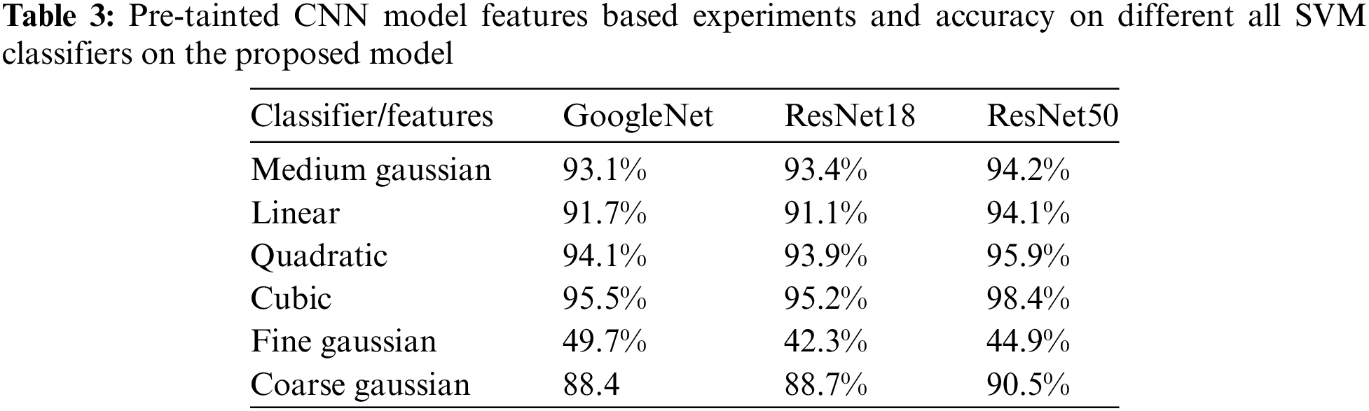
Fig. 4 shows the confusion matrix of Cubic SVM, that shows height results on the proposed model.

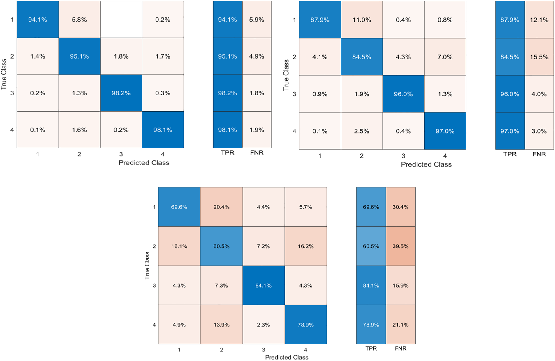
Figure 4: Confusion matrix of Cubic SVM as presented in Table 2

In Table 4, the proposed brain tumor classification model has demonstrated superior performance with a Macro F1-Score of 96.44%, a Macro Recall of 96.37%, and a slightly higher Macro F1-Score of 96.51% on Cubic SVM. These metrics collectively signify its exceptional accuracy, reliability, and balanced classification capabilities. Notably, the model showcases strong recall, minimizing the risk of missing actual brain tumor cases. Its consistency is shown from closely aligned Macro F1-Scores, reinforcing its reliability across different evaluation metrics. Graphic representation is presented in Fig. 5.

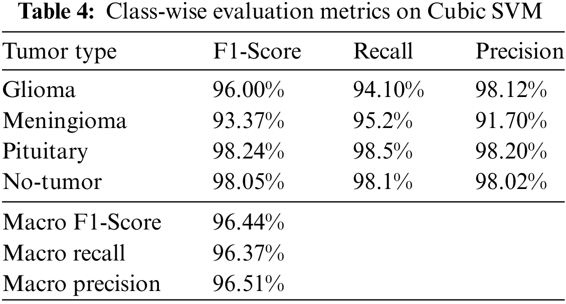
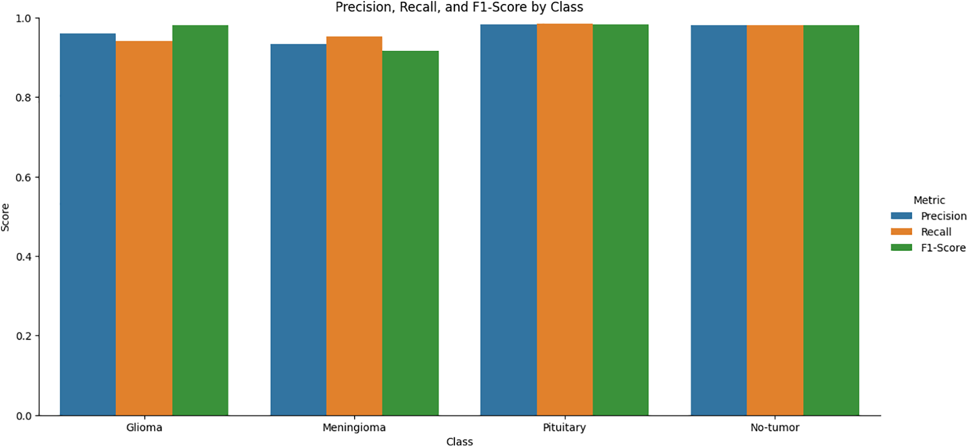
Figure 5: Graphical representation of class-wise evaluation metrics on Cubic SVM

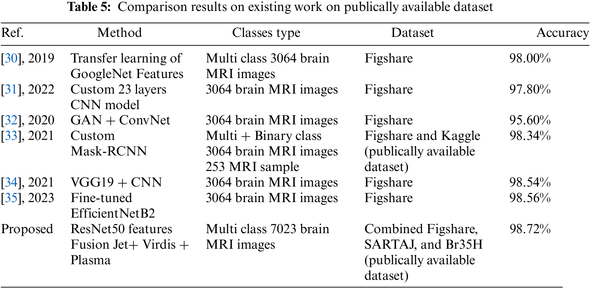
Results are compared with existing state-of-the-art methods as presented in Table 5. The main focus of the experiment’s results discussion is the notable divergence from the standard methodology used by the majority of field authors. While many authors have traditionally depended on the publicly available dataset namely the ‘Figshare’ dataset for their research, consisting of a total of 3064 images, our experiment took a more comprehensive and forward-thinking approach. We combined three distinct datasets, namely ‘Figshare’, ‘SARTAJ’, and ‘Br35H’, totaling 7023 images. This bold step was motivated by the recognition of the increasingly complex nature of real-world datasets, which often extend beyond the confines of singular, controlled datasets. The decision to combine these datasets was validated by the remarkable results achieved during the experiment. By working with a more complex dataset, our model demonstrated significantly produced accuracy, particularly when challenged with the complex nature of the combined dataset. This approach showcased the model’s robustness and capacity to handle the details of real-world data, which often exhibit variations, nuances, and complexities that transcend the boundaries of individual datasets.

5  Conclusion

In this study, we proposed a model based on color transformation which shows that the integration of color-transformed images with the progressive capabilities of deep learning, utilizing the ResNet50 architecture, has yielded significantly improved results. We conducted our experiments on a significantly more complex dataset than previous studies, and the proposed model demonstrated the ability to classify brain tumors with achieving an accuracy rate of 98.72%. This highlights the potential and effectiveness of this innovative approach, which combines state-of-the-art techniques to achieve superior results in the field of tumor classification. Data used in the article is publically available at: https://www.kaggle.com/datasets/masoudnickparvar/brain-tumor-mri-dataset.

Acknowledgement: The author extends his appreciation to Prince Sattam bin Abdulaziz University for funding this research work through the Project Number (PSAU/2023/01/24607).

Funding Statement: The research work received funding from Prince Sattam bin Abdulaziz University through the Project Number (PSAU/2023/01/24607).

Author Contributions: The authors confirm contribution to the paper as follows: Study conception, design data collection, analysis and interpretation of results, and draft manuscript preparation: F. Dahan. The author reviewed the results and approved the final version of the manuscript.

Availability of Data and Materials: The data used to support the findings of this study are available from the author upon request (f.naji@psau.edu.sa).

Conflicts of Interest: The author declares that he has no conflicts of interest to report regarding the present study.

References

1. N. A. Samee et al., “Classification framework for medical diagnosis of brain tumor with an effective hybrid transfer learning model,” Diagn., vol. 12, pp. 2541, 2022. doi: 10.3390/diagnostics12102541 [Google Scholar] [PubMed] [CrossRef]

2. S. R. Cherry, “Multimodality imaging: Beyond PET/CT and SPECT/CT,” in Semin. in Nuclear Med., 2009, pp. 348–353. [Google Scholar]

3. M. Yildirim, E. Cengil, Y. Eroglu, and A. Cinar, “Detection and classification of glioma, meningioma, pituitary tumor, and normal in brain magnetic resonance imaging using deep learning-based hybrid model,” Iran J. Comput. Sci., vol. 6, pp. 1–10, 2023. [Google Scholar]

4. M. Ali et al., “Brain tumor detection and classification using PSO and convolutional neural network,” Comput. Mater. Contin., vol. 73, no. 3, pp. 4501–4518, 2022. [Google Scholar]

5. K. Prabha, B. Nataraj, A. Karthikeyan, N. Mukilan, and M. Parkavin, “MRI imaging for the detection and diagnosis of brain tumors,” in 2023 4th Int. Conf. on Smart Electron. Commun. (ICOSEC), 2023, pp. 1541–1546. [Google Scholar]

6. L. Yuan et al., “An improved method for CFNet identifying glioma cells,” in Int. Conf. on Intell. Comput., 2023, pp. 97–105. [Google Scholar]

7. I. Decimo, G. Fumagalli, V. Berton, M. Krampera, and F. Bifari, “Meninges: From protective membrane to stem cell niche,” Am. J. Stem Cells, vol. 1, no. 2, pp. 92–105, 2012 [Google Scholar] [PubMed]

8. S. Bibi et al., “MSRNet: Multiclass skin lesion recognition using additional residual block based fine-tuned deep models information fusion and best feature selection,” Diagn., vol. 13, pp. 3063, 2023. doi: 10.3390/diagnostics13193063 [Google Scholar] [PubMed] [CrossRef]

9. M. O. Khairandish, M. Sharma, V. Jain, J. M. Chatterjee, and N. Jhanjhi, “A hybrid CNN-SVM threshold segmentation approach for tumor detection and classification of MRI brain images,” IRBM, vol. 43, no. 4, pp. 290–299, 2022. doi: 10.1016/j.irbm.2021.06.003. [Google Scholar] [CrossRef]

10. J. Naz et al., “Recognizing gastrointestinal malignancies on WCE and CCE images by an ensemble of deep and handcrafted features with entropy and PCA based features optimization,” Neural Process. Lett., vol. 55, pp. 115–140, 2023. doi: 10.1007/s11063-021-10481-2. [Google Scholar] [CrossRef]

11. A. B. Menegotto and S. C. Cazella, “Multimodal deep learning for computer-aided detection and diagnosis of cancer: Theory and applications,” in Enhanced Telemedicine and E-Health: Advanced IoT Enabled Soft Computing Framework, Swiss, Springer, Cham, 2021, pp. 267–287. [Google Scholar]

12. S. Ali, J. Li, Y. Pei, R. Khurram, K. U. Rehman and T. Mahmood, “A comprehensive survey on brain tumor diagnosis using deep learning and emerging hybrid techniques with multi-modal MR image,” Arch. Comput. Method Eng., vol. 29, pp. 4871–4896, 2022. doi: 10.1007/s11831-022-09758-z. [Google Scholar] [CrossRef]

13. S. E. Amin and M. Megeed, “Brain tumor diagnosis systems based on artificial neural networks and segmentation using MRI,” in 2012 8th Int. Conf. Inform. Syst. (INFOS), 2012, pp. MM-119–MM-124. [Google Scholar]

14. T. Tazin et al., “A robust and novel approach for brain tumor classification using convolutional neural network,” Comput. Intell. Neurosci., vol. 2021, pp. 1–11, 2021. [Google Scholar]

15. M. K. Abd-Ellah, A. I. Awad, H. F. Hamed, and A. A. Khalaf, “Parallel deep CNN structure for glioma detection and classification via brain MRI Images,” in 2019 31st Int. Conf. on Microelectron. (ICM), 2019, pp. 304–307. [Google Scholar]

16. P. Afshar, K. N. Plataniotis, and A. Mohammadi, “Capsule networks for brain tumor classification based on MRI images and coarse tumor boundaries,” in ICASSP 2019-2019 IEEE Int. Conf. on Acoustics, Speech and Signal Process. (ICASSP), 2019, pp. 1368–1372. [Google Scholar]

17. M. Nazir, F. Wahid, and S. Ali Khan, “A simple and intelligent approach for brain MRI classification,” J. Intell. Fuzzy Syst., vol. 28, pp. 1127–1135, 2015. doi: 10.3233/IFS-141396. [Google Scholar] [CrossRef]

18. L. Liu, H. Zhang, I. Rekik, X. Chen, Q. Wang and D. Shen, “Outcome prediction for patient with high-grade gliomas from brain functional and structural networks,” in Med. Image Comput. Comput.-Assist. Intervention–MICCAI 2016: 19th Int. Conf., Proc., Part II 19, Athens, Greece, Oct. 17–21, 2016, pp. 26–34. [Google Scholar]

19. A. Sawant, M. Bhandari, R. Yadav, R. Yele, and M. S. Bendale, “Brain cancer detection from MRI: A machine learning approach (tensorflow),” Brain, vol. 5, pp. 2089–2094, 2018. [Google Scholar]

20. I. Soesanti, M. Avizenna, and I. Ardiyanto, “Classification of brain tumor MRI image using random forest algorithm and multilayers perceptron,” J. Eng. Appl. Sci., vol. 15, pp. 3385–3390, 2020. [Google Scholar]

21. M. I. Sharif, M. A. Khan, M. Alhussein, K. Aurangzeb, and M. Raza, “A decision support system for multimodal brain tumor classification using deep learning,” Complex Intell. Syst., vol. 8, pp. 1–14, 2021. [Google Scholar]

22. M. A. Khan et al., “Multimodal brain tumor classification using deep learning and robust feature selection: A machine learning application for radiologists,” Diagn., vol. 10, no. 8, pp. 565, 2020. doi: 10.3390/diagnostics10080565 [Google Scholar] [PubMed] [CrossRef]

23. A. Saleh, R. Sukaik, and S. S. Abu-Naser, “Brain tumor classification using deep learning,” in 2020 Int. Conf. Assist. Rehabil. Technol. (iCareTech), 2020, pp. 131–136. [Google Scholar]

24. F. J. Díaz-Pernas, M. Martínez-Zarzuela, M. Antón-Rodríguez, and D. González-Ortega, “A deep learning approach for brain tumor classification and segmentation using a multiscale convolutional neural network,” Healthcare, vol. 9, no. 2, pp. 153, 2021. doi: 10.3390/healthcare9020153 [Google Scholar] [PubMed] [CrossRef]

25. A. Çinar and M. Yildirim, “Detection of tumors on brain MRI images using the hybrid convolutional neural network architecture,” Med. Hypotheses, vol. 139, pp. 109684, 2020. doi: 10.1016/j.mehy.2020.109684 [Google Scholar] [PubMed] [CrossRef]

26. A. Anil, A. Raj, H. A. Sarma, N. Chandran, and P. L. Deepa, “Brain tumor detection from brain MRI using deep learning,” Int. J. Innov. Res. Appl. Sci. Eng. (IJIRASE), vol. 3, pp. 458–465, 2019. [Google Scholar]

27. C. Jun, “Brain tumor dataset figshare,” Dataset, 2017. doi: 10.6084/m9.figshare.1512427.v5. [Google Scholar] [CrossRef]

28. M. A. Gómez-Guzmán et al., “Classifying brain tumors on magnetic resonance imaging by using convolutional neural networks,” Electron., vol. 12, no. 4, pp. 955, 2023. doi: 10.3390/electronics12040955. [Google Scholar] [CrossRef]

29. M. Nickparvar, “Brain tumor MRI dataset,” vol. 1, 2021. doi: 10.34740/kaggle/dsv/2645886. [Google Scholar] [CrossRef]

30. S. Deepak and P. Ameer, “Brain tumor classification using deep CNN features via transfer learning,” Comput. Biol. Med., vol. 111, pp. 103345, 2019. doi: 10.1016/j.compbiomed.2019.103345 [Google Scholar] [PubMed] [CrossRef]

31. M. S. I. Khan et al., “Accurate brain tumor detection using deep convolutional neural network,” Comput. Struct. Biotechnol. J., vol. 20, pp. 4733–4745, 2022. doi: 10.1016/j.csbj.2022.08.039 [Google Scholar] [PubMed] [CrossRef]

32. N. Ghassemi, A. Shoeibi, and M. Rouhani, “Deep neural network with generative adversarial networks pre-training for brain tumor classification based on MR images,” Biomed. Signal Process., vol. 57, pp. 101678, 2020. doi: 10.1016/j.bspc.2019.101678. [Google Scholar] [CrossRef]

33. M. Masood et al., “A novel deep learning method for recognition and classification of brain tumors from MRI images,” Diagn., vol. 11, no. 5, pp. 744, 2021. doi: 10.3390/diagnostics11050744 [Google Scholar] [PubMed] [CrossRef]

34. A. M. Gab Allah, A. M. Sarhan, and N. M. Elshennawy, “Classification of brain MRI tumor images based on deep learning PGGAN augmentation,” Diagn., vol. 11, pp. 2343, 2021. doi: 10.3390/diagnostics11122343 [Google Scholar] [PubMed] [CrossRef]

35. F. Zulfiqar, U. I. Bajwa, and Y. Mehmood, “Multi-class classification of brain tumor types from MR images using EfficientNets,” Biomed Signal Process., vol. 84, p. 104777, 2023. doi: 10.1016/j.bspc.2023.104777. [Google Scholar] [CrossRef]