A Study on Optimizing the Double-Spine Type Flow Path Design for the Overhead Transportation System Using Tabu Search Algorithm

1  Introduction

Vehicles or shuttles find common application across various industrial sectors for resolving internal transportation challenges. In the past, vehicle-based transportation was primarily associated with facility layouts. However, today, numerous research centers necessitate a zero-footprint approach to maintain clean rooms, and many facilities boast intricate machinery layouts that require an efficient materials handling system. Consequently, there is a growing need for OTSs to facilitate the movement of materials between stations. Numerous research efforts and systems pertain to OTSs, including Telelift’s transport system, OTSs designed for semiconductor fabrication plants [1–5], multi-station, multi-container transport systems [6], and others. OTSs are designed to operate independently of fleet layout considerations [5], making them ideal for managing materials without disrupting floor activities. Furthermore, OTSs can alleviate staff shortages by automating material transport, allowing personnel to focus on their core tasks rather than manual material handling [7].

Although the transport system is known as OTSs, it can still be considered a familiar transportation system. Consequently, its design can be categorized as a type of Automated Guided Vehicle system (AGVs). Related research has identified several problems in designing transportation systems [8–10], including issues such as: (1) facility layout design (FLD); (2) estimating the number of vehicles required; (3) vehicle scheduling; (4) idle-vehicle positioning; (5) battery management; (6) vehicle routing; (7) deadlock resolution. Each of these issues plays a vital role in the design and control of the transportation system, with FLD being of strategic importance. FLD involves choosing the system’s layout type, pick-up and drop-off points, and Flow Path Design (FPD) [10]. The performance of the transportation system is profoundly affected by FPD due to its significant influence on routing and dispatching rules. Conversely, a poorly designed flow path can lead to congestion and deadlock during deliveries [11].

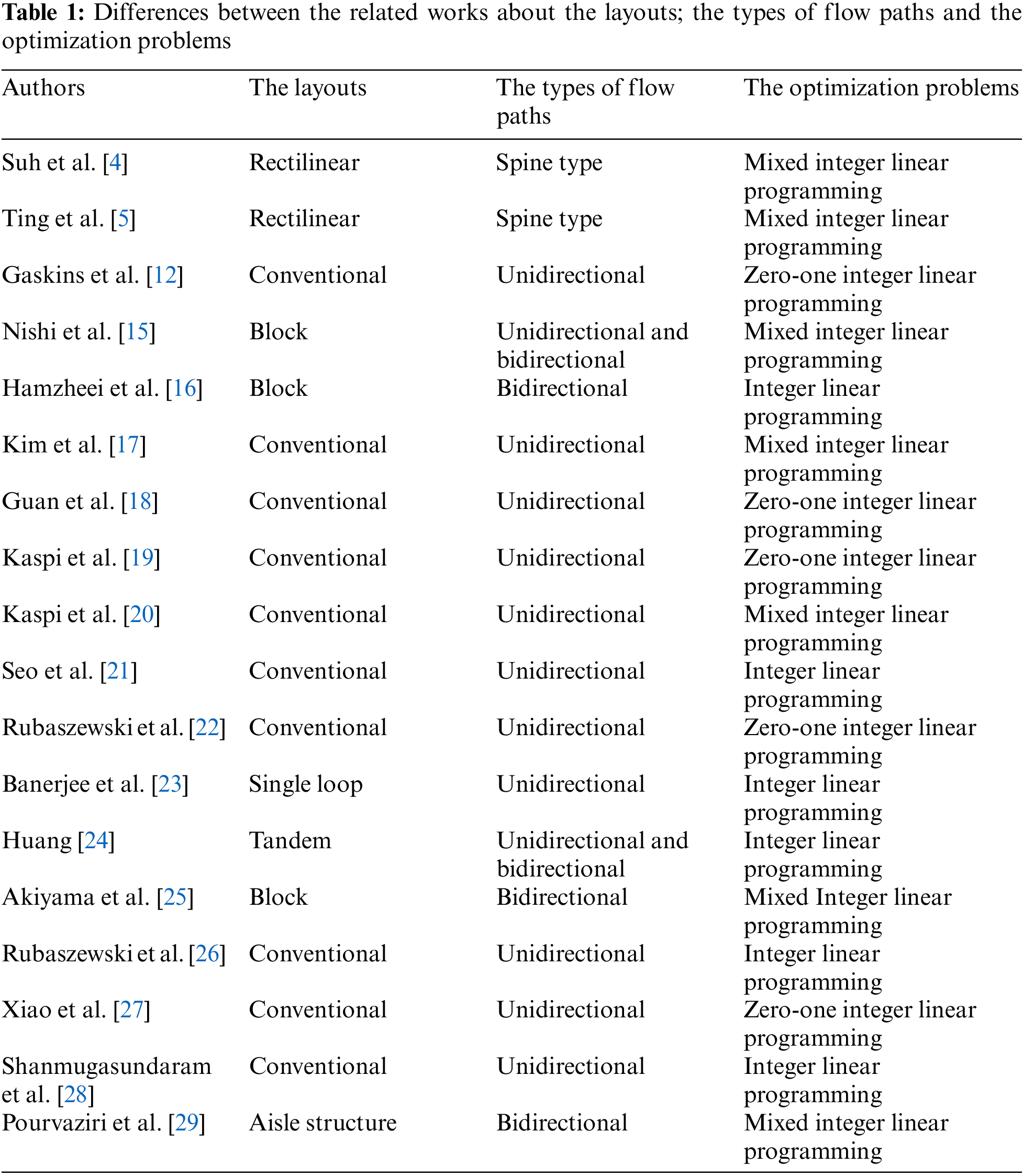
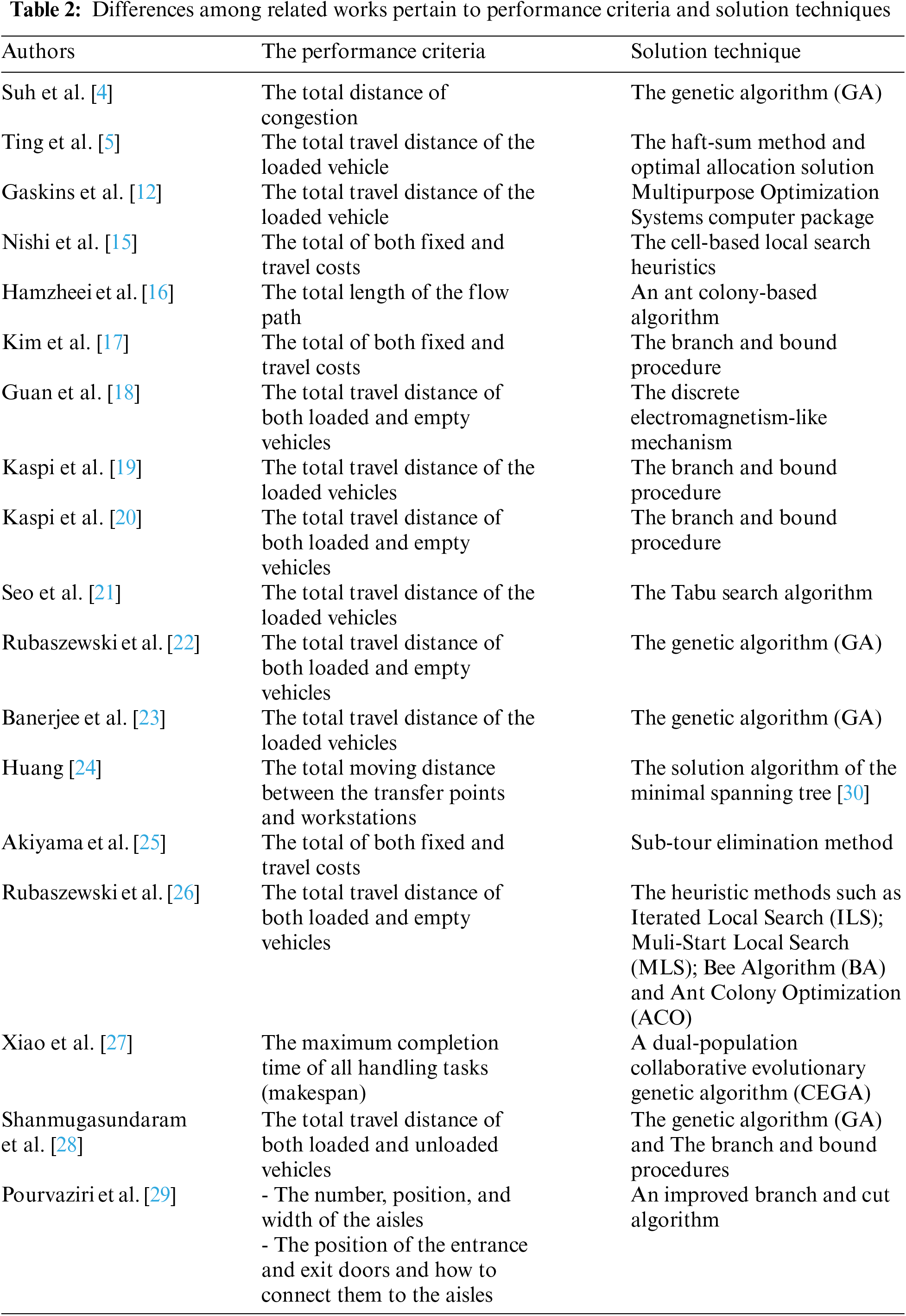
The concept of Flow Path Design (FPD) was initially introduced in 1987 by Gaskin et al. [12]. This introduction sparked the development of numerous studies aimed at optimizing Flow Path Design (FPD). From related research, several basic features of how to optimize flow path design have emerged, including (1) layout; (2) flow path type; (3) optimization problems; (4) performance criteria; (5) input; and (6) methods to solve the objective function. The three most used layouts for designing flow paths are the conventional, single loop, and tandem layouts. Additionally, the rectilinear flow layout holds promise for future expansion of Overhead Transportation Systems (OTSs) [5], while the block layout format is currently under study [13–16]. Selecting the flow path type involves determining the direction for each path, which can be unidirectional, bidirectional, or multiple-lane flow path types. It is worth noting that bidirectional flow paths can reduce the total travel distance of vehicles; however, it is important to be aware that they may also lead to congestion and operational deadlock during transportation [8–10]. Most researchers construct objective functions to present the problem, aiming to optimize one or more criteria related to system operation. The most common method for modeling these objectives is mathematical programming. Performance criteria used for optimization include the total distance of both loaded and empty flows; the shortest path; the fixed cost such as path construction, space cost, and cost of control [17]; the total moving distance between the transfer points and workstations (tandem type); the total distance of congestion; and more. Optimization problems typically require two parameters: The facility layout and the from-to chart of material flows. Finally, methods for solving objective functions can be mathematical, simulation-based, or heuristic. The following tables (Tables 1 and 2) below provide summaries of studies employing various methods related to optimizing Facility Layout Design (FLD), in accordance with the basic features mentioned above.

After conducting a literature review, it becomes evident that there is a wide range of methods available for optimizing Flow Path Design (FPD). Some commonly used methods to optimize FPD include exact mathematical analysis models, such as branch and bound, or simulation methods. However, it can be time-consuming when dealing with scaled-up problems with a large number of variables [15,18]. On the other hand, most related studies tend to focus solely on optimizing the loaded travel distance of vehicles, particularly for conventional types with layouts attached to the ground. However, there are certain critical issues that have not received as much research attention, namely, (1) optimizing the FPD for OTSs, and (2) minimizing the total travel distance of empty flows. Hence, this research aims to bridge this gap by proposing a metaheuristic method along with transportation methods to optimize the FPD for OTSs. The primary objective is to minimize the combined travel distance of both loaded and empty flows, ensuring efficient cargo delivery from pick-up stations to delivery stations. This system is designed to allow single-load transportation of vehicles along a designated flow path. For future expansion considerations, the double-spine layout type has been chosen. The proposed approach leverages the Tabu Search algorithm, the North-West Corner method, the Stepping-Stone Method, and the Rectilinear Minisum Location Problem as the appropriate tools to address these optimization problems.

The organization of this manuscript is as follows. The proposed problem is described in Section 2. In Section 3, the numerical analysis will be discussed. Then Section 4 will assess the results. The conclusion of the research will be discussed in Section 5.

2  Problem Description

2.1 Optimize the Double-Spine Type Layout Design

The spine layout is commonly used for systems with future expansion needs, offering two main forms: Single-spine and double-spine. In the single-spine layout, there is one main branch (which can be either X-spine or Y-spine), with load ports or stations connecting to the spine as sub-branches. Similarly, the double-spine layout comprises two perpendicular single main branches (the X-spine and Y-spine). Each station will only connect to one of the two main spines (not both simultaneously). Figs. 1a and 1b below introduce the basic single-spine and double-spine layouts, respectively.

Figure 1: (a) The single-spine layout (X and Y types), (b) The double spine layout

The spine model is positioned in the layout referred to as the rectilinear layout. In this layout, the X-spine is positioned at coordinates of x=x0, and the Y-spine is positioned at coordinates y=y0. Each station is represented as a point with known coordinates, denoted as Pi(ai,bi), as shown in Fig. 1a. The station positions in the coordinate system are illustrated in Fig. 2, which is employed in this research.

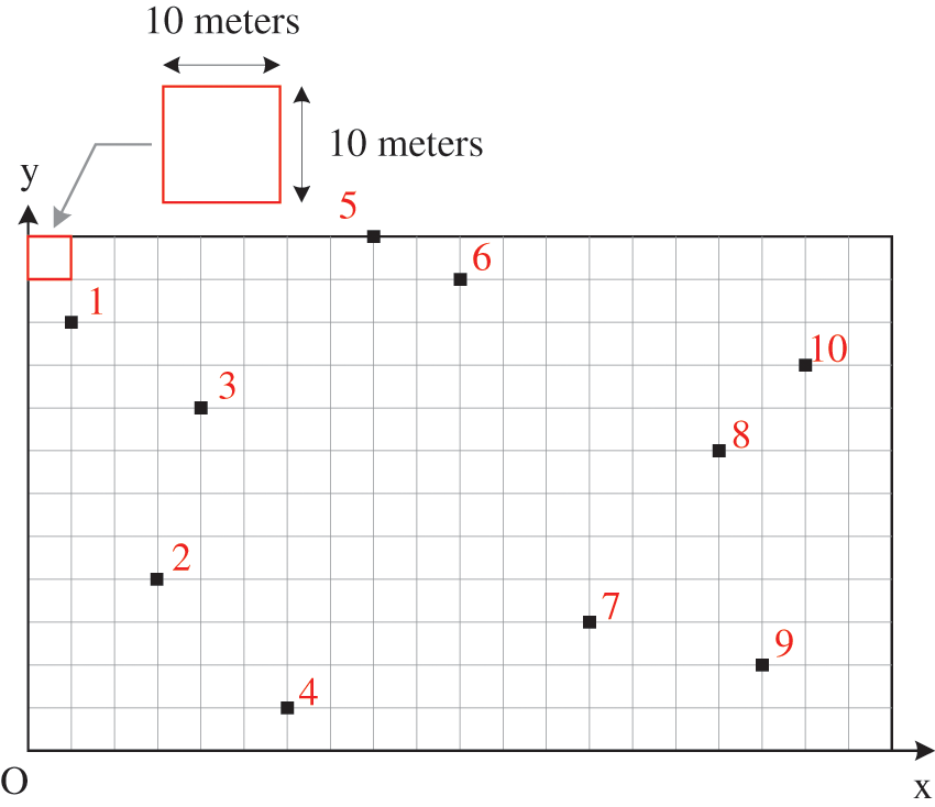
Figure 2: The 10 stations are arranged in a rectilinear layout

As mentioned earlier, each point is only connected to one main branch. Therefore, the stations are divided into two separate sets, respectively:

SX: The set of points Pi associated with the X-spine.

SY: The set of points Pj associated with the Y-spine.

Based on Figs. 1a and 1b, we derive the general formula for the rectilinear distance between two points Pi and Pj as follows:

dij=|ai−x0|+|bi−bj|+|x0−aj|: When Pi and Pj associated with the X-spine.

dij=|bi−y0|+|ai−aj|+|y0−bj|: When Pi and Pj associated with the Y-spine.

dij=|ai−x0|+|bi−y0|+|x0−aj|+|bj−y0|: When Pi associated with the X-spine and Pj associated with the Y-spine.

Denoting that the material flows from the Pi to Pj as fij. Because the empty travel flows (the travel that the vehicles do not deliver the loads) are considered, we denote eij to represent the empty travel from Pi to Pj. The transportation method can be applied to optimal the empty travel [31].

The integer programming model is employed to formulate the objective function for minimizing the total travel distance among the 10 stations. However, it is essential to divide the objective function into three parts: (1) the paths that include flows among the points in SX; (2) the paths that encompass flows among the points in SY; and (3) the paths that involve flows among the points in both sets SX and SY.

The objective function aims to minimize the total travel distance of both loaded and empty flows among the points in SX:

∑i=SX∑j=SXfijdij+∑i=SX∑j=SXeijdij=∑i=SX∑j=SX(fij+eij)(|ai−x0|+|bi−bj|+|x0−aj|)(1)

The objective function aims to minimize the total travel distance of both loaded and empty flows among the points in SY:

∑i=SY∑j=SYfijdij+∑i=SY∑j=SYeijdij=∑i=SY∑j=SY(fij+eij)(|bi−y0|+|ai−aj|+|y0−bj|)(2)

The objective function aims to minimize the total travel distance of both loaded and empty flows among the points from two sets SX and SY:

∑i=SX∑j=SYfijdij+∑i=SY∑j=SXfijdij+∑i=SX∑j=SYeijdij+∑i=SY∑j=SXeijdij=∑i=SX∑j=SY(fij+eij)(|ai−x0|+|bi−y0|+|x0−aj|+|bj−y0|)+∑i=SY∑j=SX(fij+eij)(|ai−x0|+|bi−y0|+|x0−aj|+|bj−y0|)(3)

According to Ting et al. [5] and Tompkins et al. [32], the optimization of x0 and y0, as well as the branching of stations into two sets SX and SY can be solved separately. Consequently, three distinct subproblems need to be addressed: Optimizing the x0 and y0 values, and branching the stations.

Subproblem 1: Optimize x0—This involves considering the flow between the points in SX as Eq. (1) and the flow among the points from both sets SX and SY as Eq. (3):

Zx0=∑i=SX∑j=SX(fij+eij)(|ai−x0|+|x0−aj|)+∑i=SX∑j=SY(fij+eij)(|ai−x0|+|x0−aj|)+∑i=SY∑j=SX(fij+eij)(|ai−x0|+|x0−aj|)=∑i=1n∑j=1n(fij+eij)(|ai−x0|+|x0−aj|)=∑i=1n(wi+zi)|ai−x0|(4)

Subproblem 2: Optimize y0—This involves considering the flow between the points in SY as Eq. (2) and the flow among the points from both sets SX and SY as Eq. (3):

Zy0=∑i=SY∑j=SY(fij+eij)(|bi−y0|+|y0−bj|)+∑i=SX∑j=SY(fij+eij)(|bi−y0|+|y0−bj|)+∑i=SY∑j=SX(fij+eij)(|bi−y0|+|y0−bj|)=∑i=1n∑j=1n(fij+eij)(|bi−y0|+|y0−bj|)=∑i=1n(wi+zi)|bi−y0|(5)

Subproblem 3: Branching the stations–This subproblem involves considering all the flows in Eqs. (1)–(3):

Zx0y0=∑i=SX∑j=SX(fij+eij)(|ai−x0|+|bi−bj|+|x0−aj|)+∑i=SY∑j=SY(fij+eij)(|bi−y0|+|ai−aj|+|y0−bj|)+∑i=SX∑j=SY(fij+eij)(|ai−x0|+|bi−y0|+|x0−aj|+|bj−y0|)+∑i=SY∑j=SX(fij+eij)(|ai−x0|+|bi−y0|+|x0−aj|+|bj−y0|)(6)

As mentioned earlier, the objective functions represented by Eqs. (4) and (5) can be solved independently. The Rectilinear Minisum Location Problem [32] can be applied to optimize these two values, x0 and y0. It is important to note that wi represents the total loaded travel flows to and from station i, and zi represents the total empty travel flows to and from station i. Additionally, because |ai−aj| and |bi−bj| are constant, they can be removed from Eqs. (4) and (5) during the analysis.

2.2 The Tabu Search (TS) Algorithm and the Transportation Methods

The TS algorithm is a metaheuristic method that relies on an initial feasible solution. Once the initial feasible solution is obtained, a search algorithm is employed to identify the admissible neighborhood and replace the current solution with the best-improving neighborhood. Notably, one unique feature of TS is its ability to accept non-improving moves [33]. In this study, the TS algorithm will be characterized by two factors: Short-term memory and long-term memory. The TS algorithm is applied to handle the objective function represented by Eq. (6).

The function represented by Eq. (6) is converted into a binary integer programming form, as demonstrated in Eq. (7). In Eq. (7), dijx and dijy denote the distance between two stations intra X-spine and Y-spine, while dijz and dijw represent the distance between two stations inter X-spine and Y-spine. The formulas for dijx, dijy, dijz, dijw are provided in Eqs. (8) to (11).

Z=∑i=1n∑j=1n(fij+eij)(dijx+dijy+dijz+dijw)(7)

Two decision variables xi and yi, where i∈{1,2,3,…,10}, correspond to the branches that connect to X-spine and Y-spine, respectively. When xi=1, it signifies a branch from station i that links with the X-spine, and when yi=1, it indicates a branch from station i that connects to the Y-spine, and vice versa. To ensure that each station is exclusively associated with either the X-spine or Y-spine, a constraint is necessary, as depicted in Eq. (12).

Thus:

dijx=(xi+xj−1)(|ai−x0|+|bi−bj|+|x0−aj|)≥0(8)

dijy=(yi+yj−1)(|bi−y0|+|ai−aj|+|y0−bj|)≥0(9)

dijz=(xi+yj−1)(|ai−x0|+|bi−y0|+|x0−aj|+|bj−y0|)≥0(10)

dijw=(yi+xj−1)(|ai−x0|+|bi−y0|+|x0−aj|+|bj−y0|)≥0(11)

xi+yi=1(12)

To execute the TS, an initial solution that represents the existence of associated branches with a binary string C must be determined. In this binary string, the bit 0 or 1 signifies the presence of branches from stations to either the X-spine or Y-spine. A value of 1 indicates that the station is connected to the X-spine, corresponding to xi=1 and yi=0. Conversely, a value of 0 denotes that the station is linked to the Y-spine, resulting in xi=0 and yi=1.

Assuming the initial possible solution as the current and the best solution to the problem, the next stage of TS will involve searching for neighbors by making changes bit-by-bit to the binary string C to achieve admissible move. In TS, “move” refers to transitioning from the current solution to the best-improved solution. For all admissible neighbors, the total travel distance is computed using Eq. (7) to identify the best-improving move, which is then executed a move.

Since this research considers empty travel flows, it is necessary to determine the empty travel matrix. According to Muckstadt and Maxwell [34], the net vehicle flow of each station, denoted as NF(i), is defined as NF(i)=∑jfji−∑jfij. Here, ∑jfji represents the total travel distance of loaded flows to station i, and ∑jfij represents the total travel distance of loaded flows from station i. On the other hand, the supply constraint for each delivery station, denoted as Sm, and the demand constraint for each pick-up station, denoted as Rl, are defined in Eqs. (13) and (14) based on the net flow equation. In this study, the transportation method is utilized to optimize the empty travel matrix for this system.

Sm={∑lflm−∑lfml∑lflm−∑lfml>00∑lflm−∑lfml≤0(13)

Rl={∑mflm−∑mfml∑mflm−∑mfml>00∑mflm−∑mfml≤0(14)

The variable eij denotes the quantity of empty travel flows of the vehicle from station i to station j. According to Muckstadt et al. [34], if the net vehicle flow NF(i) is non-negative, then ∑jeij=NF(i) and ∑jeji=0. Conversely, if the net vehicle flow NF(i) is negative, then ∑jeji=|NF(i)| and ∑jeij=0. In these equations, ∑jeij is the total of empty travel flows from node i, and ∑jeji is the total of empty travel flows to node i.

The transportation method requires a distance matrix among the 10 stations and the net vehicle flow for each station. Using this distance matrix and the net vehicle flows, the matrix of empty travel flows can be calculated using transportation methods. Two methods are applied, namely the North-West Corner method and the Stepping-Stone Method [31]. The North-West Corner method can be summarized as follows:

Step 1: At the position (1,1)—the North-West Corner, allocate as much as possible the flow value. It depends on the supply constraint—Sm, and the demand constraint—Rl. The assignment of supply and demand constraints of each station is Sm(1) to Sm(n), and Rl(1) to Rl(n).

Step 2: There are 3 cases.

Step 2.a: If Sm(1)<Rl(1), the value at position (1,1) is set to Sm(1). Consequently, column 1 is disregarded. Meanwhile, Rl(1) becomes (Rl(1)−Sm(1)), and position (1,2) is taken into consideration.

Step 2.b: If Sm(1)>Rl(1), the value at position (1,1) is set to Rl(1). Consequently, the row 1 is disregarded. Meanwhile, Sm(1) becomes (Sm(1)−Rl(1)), and position (2,1) is taken into consideration.

Step 2.c: If Sm(1)=Rl(1), the value at position (1,1) is set to both Sm(1) and Rl(1). Consequently, both column 1 and row 1 are disregarded. Next, position (2,2) is taken into consideration.

Step 3: Continue this process until reaching the position (n,n), which is the South-East Corner.

The initial feasible matrix of empty travel flows can be obtained using the North-West Corner method. Subsequently, by applying the Stepping-Stone Method, the matrix of empty travel flows with the minimum total travel distance can be determined. The conditions for using this method are: (1) the number of allocations in the initial feasible solution is 2n+1, where n is the number of stations; and (2) the allocations are independent. The Stepping-Stone Method can be summarized as follows:

Step 1: Define the initial feasible matrix of empty travel flows using the North-West Corner method.

Step 2: Examine the conditions mentioned above for the initial feasible matrix. Following that, evaluate all unoccupied positions and replace them with other occupied positions to achieve a more optimal solution. The replacement process can be handled as follows:

Step 2.1: Select an unoccupied position.

Step 2.2: Determine a closed loop through at least 3 occupied positions starting from this chosen position. The direction of the closed loop is not significant as it yields the same solution.

Step 2.3: At each corner of the closed loop, assign either a (+) or (–) sign, beginning with a (+) for the unoccupied position.

Step 2.4: Each corner of the closed loop corresponds to a cost (distance between the 2 stations). Calculate the net changes in cost for the closed loop using the assigned signs at each corner. The net change in cost is given by c1∗−c2+c3−c4, where c1∗ is the cost of the unoccupied position.

Step 2.5: Repeat steps 2.1 to 2.4 for all unoccupied positions.

Step 3: The matrix of empty travel is considered optimal if all net changes in cost are greater than or equal to zero, and the process concludes at this point. Otherwise, proceed to step 4.

Step 4: If there is more than one net change in cost that is negative, select the closed loop with the most negative value. If multiple net changes in costs have the same negative value, choose the closed loop that allows for more flow transition at the minimum cost.

Step 5: Within the chosen closed loop, replace the flow of an unoccupied position with a value from an occupied position, maximizing this replacement as much as possible.

Step 6: Return to step 2 and continue the process until all net change values are greater than or equal to zero.

As mentioned earlier, we will utilize two fundamental aspects of the TS: Short-term memory and long-term memory. In this research, static memory with a fixed Tabu tenure T is employed for short-term memory. This implies that if station a has a value b (0 or 1) denoted as [a,b] since the latest move, then after the next T iteration, the value [a,b] will not be accepted. Short-term memory is thus utilized to prevent the solution from getting stuck in local optima and encourages exploration [33]. On the other hand, long-term memory involves counting the frequency of repetition of [a,b], denoted as F[a,b]. This process of tracking the entire search is known as long-term memory. In the case of non-improving moves, the values of the objective function Z will increase proportionally with the repetition frequency F[a,b] and a penalty factor ρ. This reduces the weight given to checking non-improving moves in subsequent iterations, promoting diversity in the TS algorithm [33]. The iterative process continues until the stopping conditions are met. As suggested by Seo et al. [21], these stopping conditions can include reaching the maximum number of iterations or failing to improve the solution beyond a certain threshold within a set number of iterations. These two criteria are also applied in this research. Additionally, an aspiration criterion will be used to accept neighbors in the Tabu list if the solution is better than the current best solution [33].

The TS algorithm applied for optimizing the FPD can be illustrated as follows:

Step 1: Find an initial possible solution and assign it to both the current solution and the current best solution, denoting Cbest=Ccur=Cinit. Calculate Zinit based on the value of Cinit, then assign it to Zcur and Zbest. Begin the process with an iteration count of 0, denoted as niteration=0 and nnonimpr=0.

Step 2: Change bit-by-bit of Ccur to generate neighbor solutions. Evaluate all neighbors using short-term and long-term memory to determine admissible neighbors:

Step 2.1: Calculate Zneighbor for each neighbor.

Step 2.2: If the number of iterations since the latest move to the neighbor is less than the Tabu tenure value T, and the aspiration criterion is not met (Zneighbor>Zbest), reject the neighbor and return to the beginning of step 2. Otherwise, include the neighbor in the set of admissible neighbors and proceed to step 2.3. This step utilizes short-term memory.

Step 2.3: If the Zneighbor−Zbest≥0, set Zneighbor=Zneighbor+ρ.F[a,b]. This means that for non-improving moves, the value of the objective function Z will increase proportionally with the repetition frequency of [a,b] and the penalty factor ρ. This step involves long-term memory.

Step 3: Among the set of admissible neighbors, select the neighbor with the minimum objective function Z as the current solution. Update Ccur=Cbestimproveneighbor and Zcur=Zbestimproveneighbor. Also, update F[a,b]=F[a,b]+1 accordingly. If Zbestimproveneighbor<Zbest, assign Zbest=Zbestimproveneighbor and Cbest=Cbestimproveneighbor.

Step 4: If nnonimpr≤0 and Zbestimproveneighbor−Zcur<0, the move is considered an improving moves, and nnonimpr=nnonimpr−1. Else if nnonimpr≥0 and the Zbestimproveneighbor−Zcur>0, the move is a non-improving move, and nnonimpr=nnonimpr+1. These actions account for consecutive improving and non-improving moves. If the move is neither consecutive improving nor consecutive non-improving, set nnonimpr=0.

Step 5–Checking the stop condition: If niteration≥Niteration or nnonimpr≥Nnonimpr, terminate the search process. Otherwise, set niteration=niteration+1 and return to step 2.

3  Calculation and Numerical Analysis for Optimizing the Double-Spine Type Flow Path Design

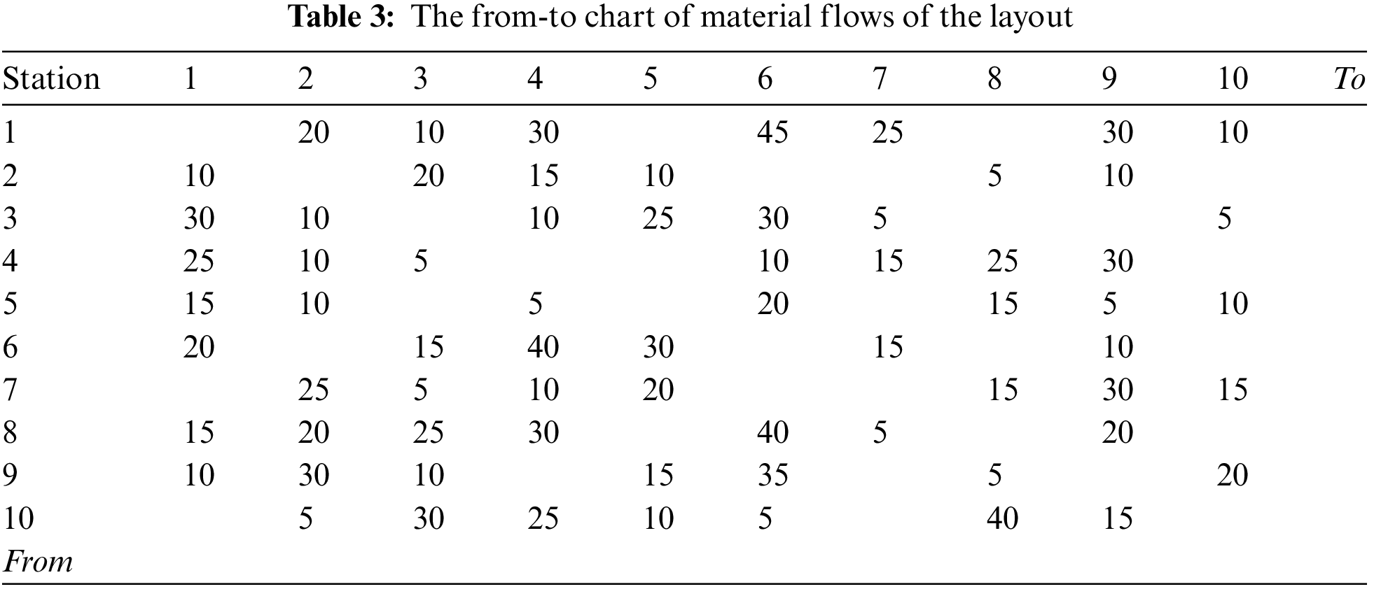
The from-to chart of material flows matrix is presented in Table 3.

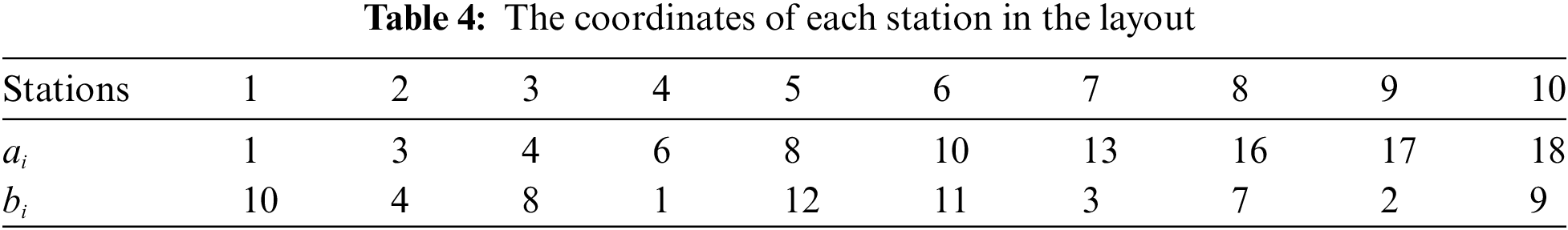
The coordinates of the 10 stations, denoted as (ai,bi), are listed in Table 4. It is important to note that in Fig. 2, each unit of length corresponds to 10 meters, simplifying calculations by using this unit.

Utilizing the data from Table 3, the net vehicle flow matrix is computed based on the vehicle flows traveling to and from station i, as shown in Table 5.

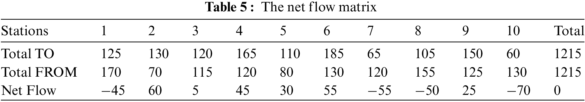
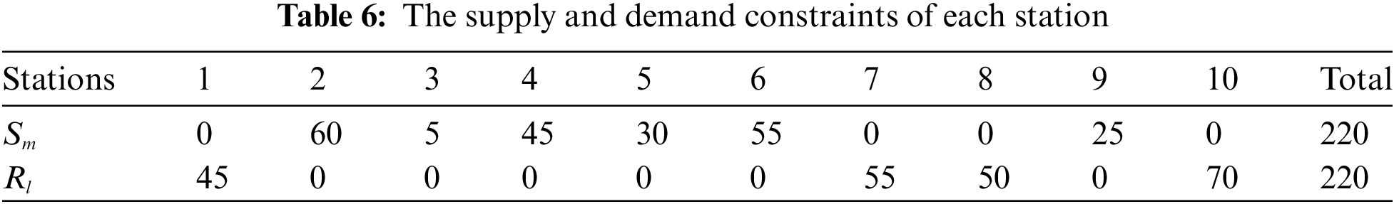
Derived from Table 5, the values for Sm and Rl are determined for each station, as depicted in Table 6.

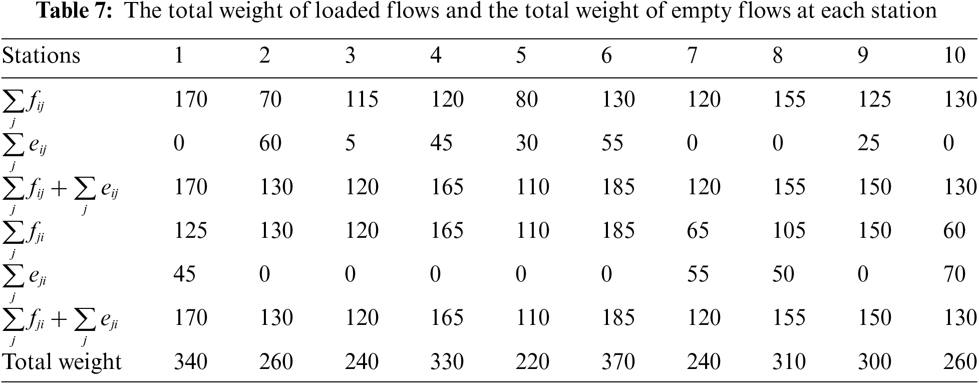
The two objective functions presented in Eqs. (4) and (5) can be addressed using “The Rectilinear Minisum Location Problem”. This method considers the total weight of both loaded and empty travel flows. The total weight is calculated as the sum of the flows to and from each station. Consequently, Table 7 has been generated, which illustrates the total weights of loaded vehicles and the total weight of empty vehicles at each station, based on the data from Tables 5 and 6.

According to Tompkins et al. [32], for functions like Eqs. (4) and (5) with piecewise linear structures, the optimal value of x0 should be such that no more than half of the total weight lies to the left of x0, and no more than half of the total weight lies to the right of x0. Similarly, the optimal value of y0 should be such that no more than half of the total weight is above y0, and no more than half of the total weight is below y0. Furthermore, each optimal solution corresponds to the coordinates of one station among the 10 stations. In other words, x0 should be equal to one of the ai values, and y0 should be equal to one of the bi values.

The following tables, Tables 8 and 9, provide the calculations for determining the optimal x0 coordinate and the optimum y0 coordinate, respectively.

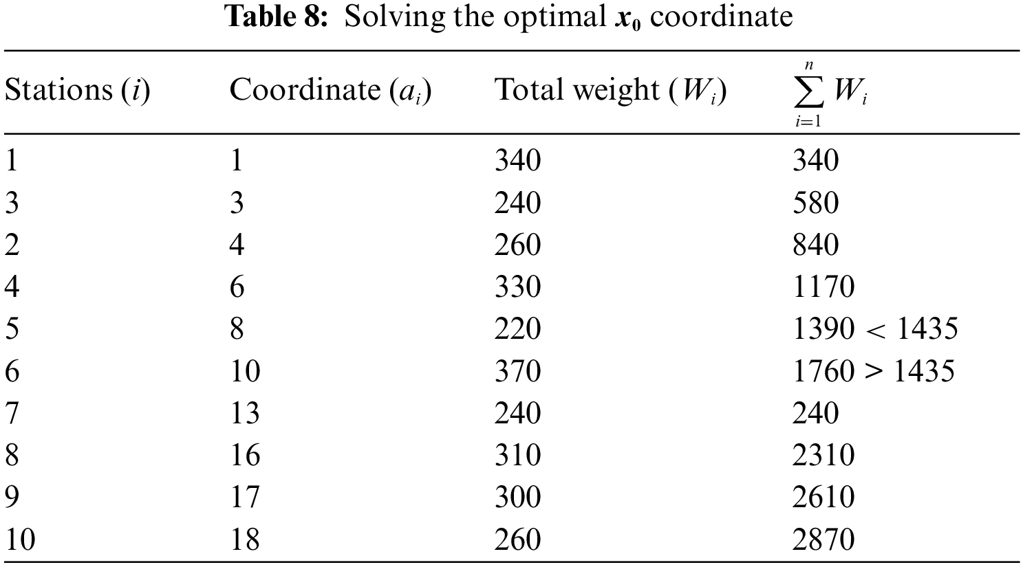
Table 8 displays the sum of the weights as 2870 and half of this sum as 1435. Based on these values, the optimal x0 coordinate is determined to be a6, which corresponds to station 6. Similarly, Table 9 reveals that the optimal y0 coordinate is b8, representing station 8. This configuration results in the placement of the X-spine at station 6 and the Y-spine at station 8, as illustrated in Fig. 3.

Figure 3: The two optimal spines in the rectilinear layout

Once the coordinates of the two spines, x0 and y0, have been determined, the next step is to branch the 8 stations to these two spines in a way that each station is connected to only one spine. To achieve this, an initial feasible solution is selected for the TS algorithm. The initial feasible solution is presented as Cinit=x10x9x8x7x6x5x4x3x2x1¯. The TS algorithm parameters include a Tabu tenure T=5, a penalty factor ρ=50, a maximum iteration count Niteration=100, and a maximum number of consecutive non-improving moves Nnonimpr=10. These parameters are determined through a trial-and-error process. A MATLAB program is used to find the optimal solution of the objective function Eq. (7) using the TS algorithm. Assure that, the initial feasible solution is set to Cinit=1101111111. With the Cinit established, the distance matrix among the 10 stations is calculated, as shown in Table 10.

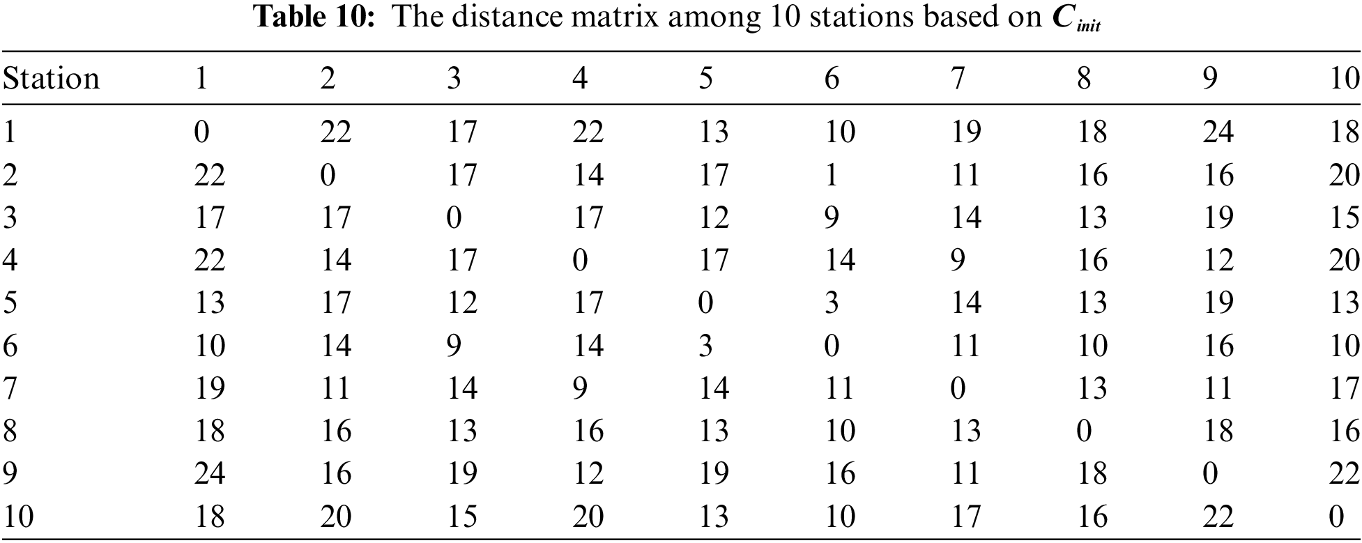
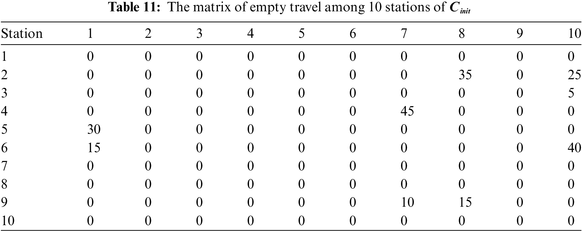
Using the transportation method, the matrix of empty travel flows is optimized based on the matrix of loaded travel flows and the distance matrix among the 10 stations. As a result, Table 11 illustrates the empty travel flows among the 10 stations for the initial feasible solution Cinit.

After 33 iterations of the TS algorithm, the optimal solution has been obtained with Cbest=0000110000 and Zbest=19360. The empty travel flows for the optimal solution are shown in Table 12. When compared to the initial feasible solution, the optimal solution, which minimizes the objective function Eq. (7), represents as an improvement ΔZ=1590. The flow path layout for Cbest=0000110000 is depicted in Fig. 4.

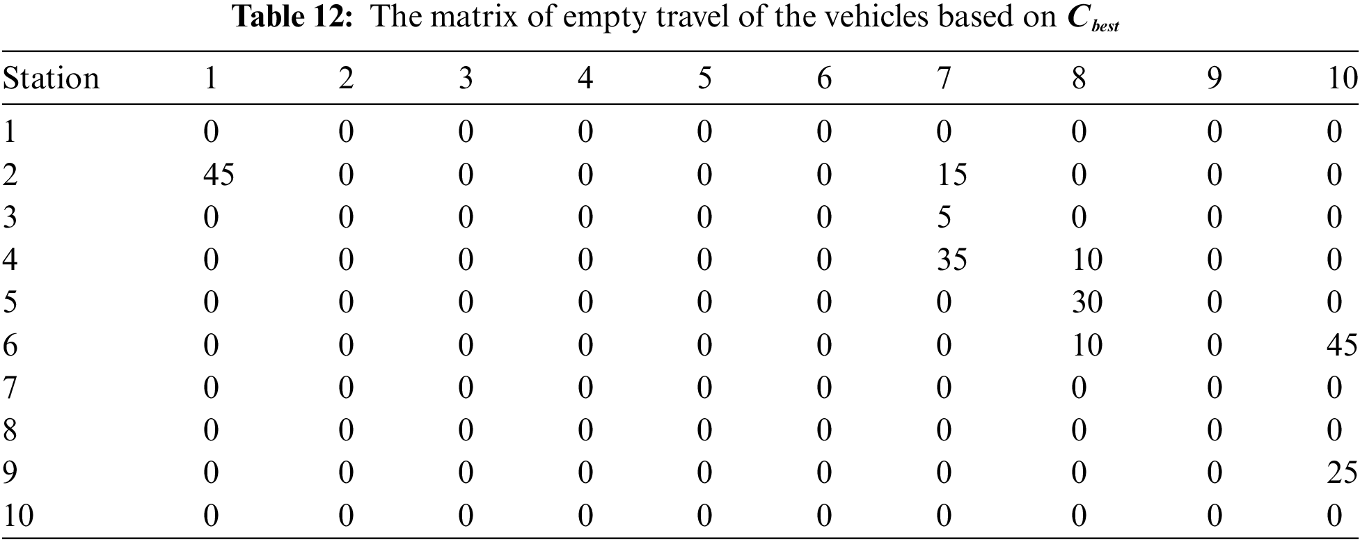
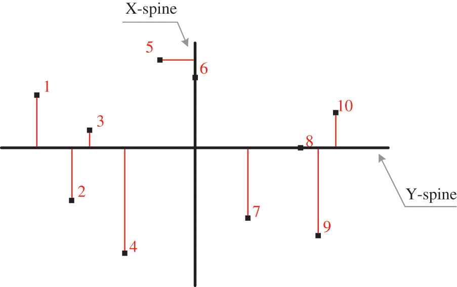
Figure 4: The optimal flow path after 33 iteration times

4  Evaluate the Numerical Analysis Results

The results obtained from the proposed method indicate a reduction in the objective function value when compared to the initial feasible solution. This reduction amounts to ΔZ=1590, which corresponds to a distance reduction of Simpr=15900(m). Fig. 5 below illustrates the graph depicting the objective function values across 100 iteration times. At the 33th iteration time, the value of the best objective function remains unchanged. Therefore, the optimal solution, Cbest=0000110000, is achieved at the 33th iteration time, with an objective function value of Zbest=19360.

Figure 5: The optimal solution by using the TS algorithm

The number of iterations required to obtain the optimal solution can vary depending on the Tabu tenure and penalty factor used in the TS algorithm. In Fig. 6, it is shown that with T=4, the optimal solution is reached after 35 iteration times. Conversely, with T=12, it takes 111 iterations to reach the optimal solution. Similarly, with T=13, it takes 225 iterations, and with T=14, it still takes after 225 iterations to reach the optimal solution. In Fig. 7, the impact of the penalty factor on the number of iterations is demonstrated. When ρ=100, the optimal solution is achieved after 29 iterations. With ρ=200, it takes 19 iterations to reach the optimal solution. When ρ=300, it takes 23 iterations, and with ρ=400, it still takes 23 iterations to reach the optimal solution. Since the number of iterations directly affects the running time of the search process, it is important to carefully consider the choice of Tabu tenure and penalty factor when applying the TS algorithm. Finding an appropriate balance between these parameters is crucial for efficient optimization.

Figure 6: The optimal solutions when changing the Tabu tenure

Figure 7: The optimal solutions when changing the penalty factor

To assess the feasibility of the proposed metaheuristic method, it was applied to the layout with 10 stations, whose research was conducted by Ting et al. [5], without considering the empty travel flows. The algorithm was configured with the following parameters: Tabu tenure T=5, penalty factor ρ=5000, maximum iteration Niteration=100, and maximum consecutive non-improving move Nnonimpr=100. The initial feasible solution was set as Cinit=1101111111 and the initial objective function value was Zinit=3825367. After 10 iteration times, the result is Cbest=0000100000 and Zbest=3039339. The result means that all 10 stations only connect with the Y-spine, and the Y-spine is located at station 8. This result is consistent with the findings of the research conducted by Ting et al. [5], demonstrating the appropriateness of the proposed method for optimizing spine flow path design. The result is shown in Fig. 8.

Figure 8: The optimal solution of the example in research [5]

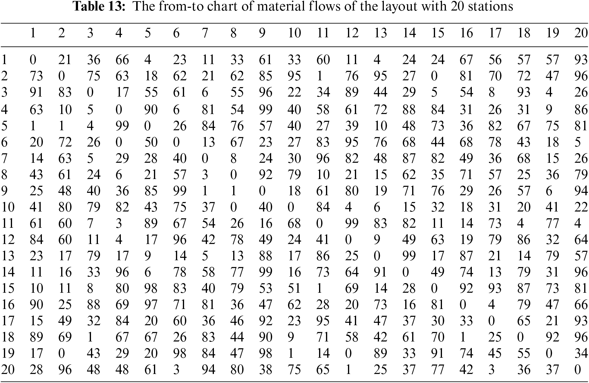
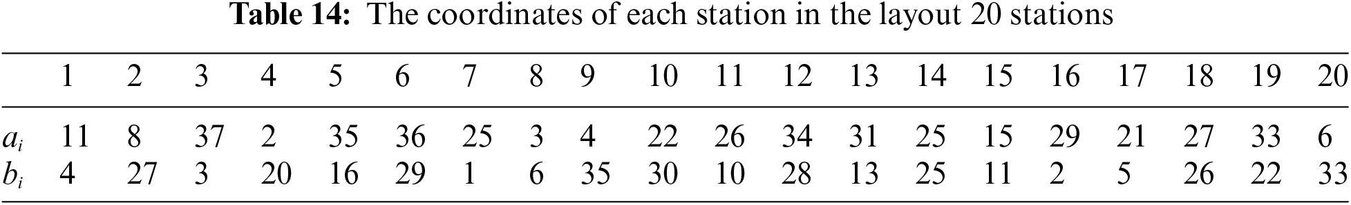
In addition, two examples of layouts with 20 stations and 30 stations were generated using our proposed method. First, with the 20-station layout, the algorithm was configured with the following parameters: Tabu tenure T=5, penalty factor ρ=1000, the maximum iteration Niteration=100, and the maximum of the consecutive non-improving move Nnonimpr=100. The optimal solution, Cbest=01111011110001110101, with an objective function value of Zbest=645908, was achieved after 74 iterations, starting with Cinit=11111111111111110111 and Zinit=656150, as shown in Fig. 9. In this layout, the X-spine and Y-spine are located at station 7 and station 4, respectively.

Figure 9: The optimal solution of the example with 20 stations

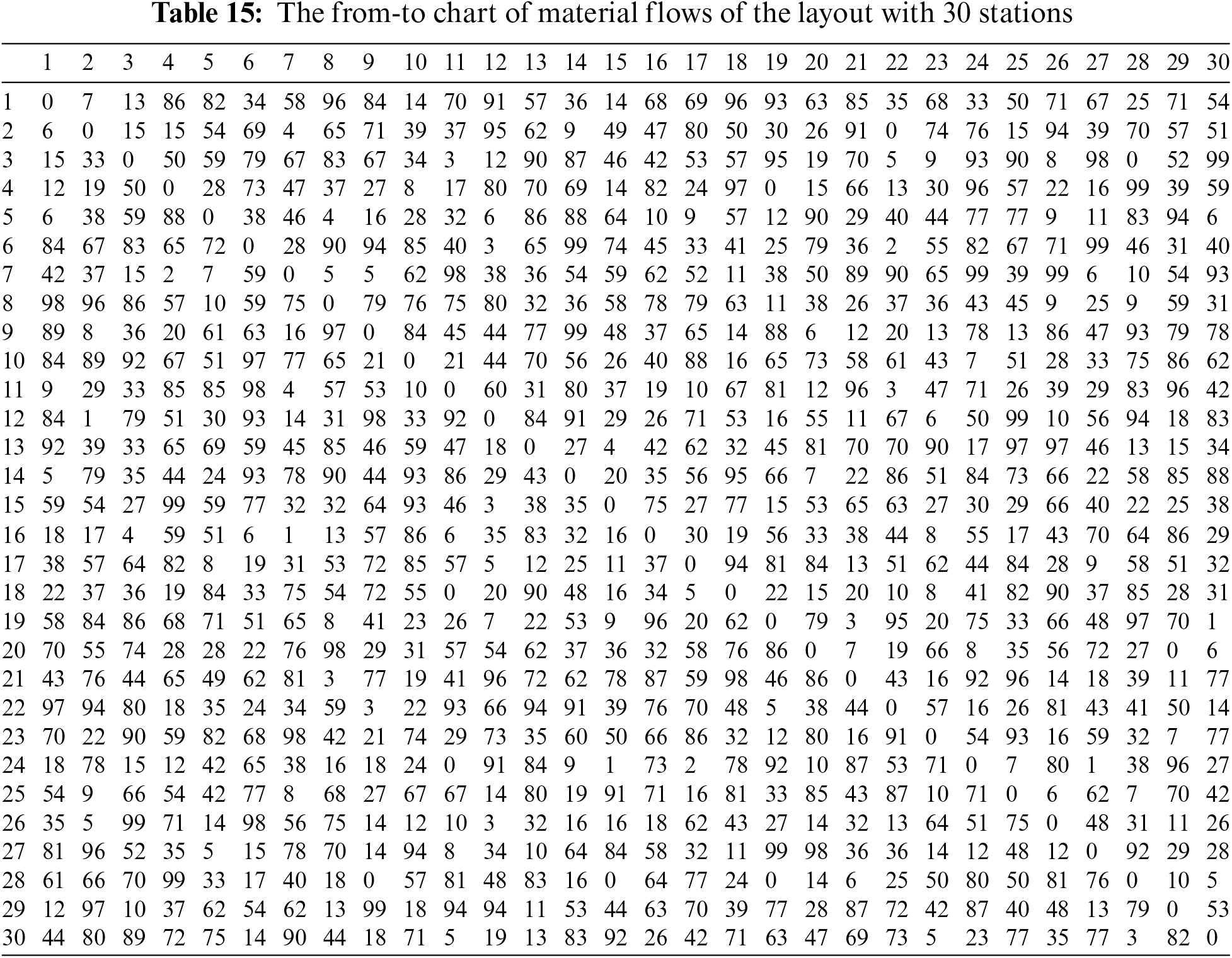
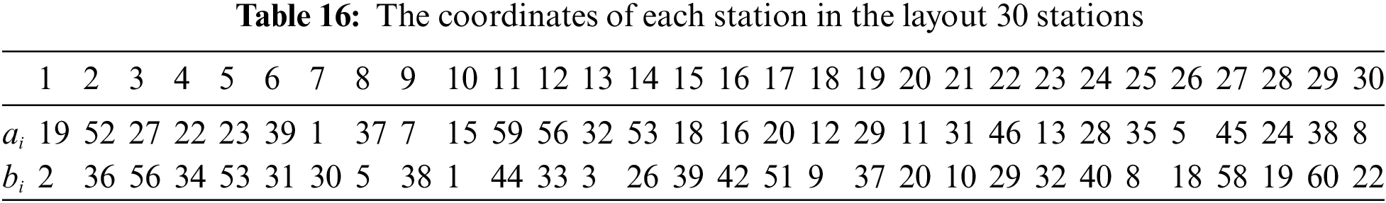
On the other hand, with the 30 stations layout, the algorithm was configured with the following parameters: Tabu tenure T=5, penalty factor ρ=5000, the maximum iteration Niteration=100, and the maximum of the consecutive non-improving move Nnonimpr=100. The optimal solution, Cbest=111111110111111101011111011101, with an objective function value of Zbest=2058714, was achieved after 34 iterations, starting with Cbest=111111111111111111111111011111 and Zinit=2068350, as demonstrated in Fig. 10. In this example, the X-spine and Y-spine are located at station 3 and station 6, respectively. The from-to chart of material flows and the coordinates table of the two examples are shown in Appendix A (Tables 13 to 16).

Figure 10: The optimal solution of the example with 30 stations

5  Conclusions

The primary objective of this research is to explore the design of OTSs, considering various critical factors outlined in the Introduction section. Among these factors, optimizing the FPD is a strategic factor that should be considered carefully. Furthermore, since this is an OTSs, the spine layout is chosen to ensure future scalability. Hence, this study places a specific emphasis on the optimization of a double-spine flow path design to minimize the total travel distance for both loaded and empty flows. Additionally, this research takes empty travel flows into account, a factor frequently overlooked in previous work. To address this, the transportation methods, including the North-West Corner and the Stepping-Stone Method, are applied to optimize empty travel flows. The Rectilinear Minisum Location Problem is also utilized to determine the locations of the two main branches, X-spine and Y-spine. Finally, the problem of branching the 10 stations into the two main branches is resolved using the TS algorithm. Key elements of this method involve specific coefficients like Tabu tenure, penalty factor, and stop criteria, which significantly impact its effectiveness.

Based on the optimal results presented in Section 4, it is evident that the suggested methods are suitable for optimizing the spine flow path design. Furthermore, to validate our methods, comparisons and examples have been conducted. The results demonstrate that the optimal solution’s value can be reduced, and the iteration count in the search process can be influenced by adjusting the coefficients used in the TS algorithm. In this study, the coefficients, including Tabu tenure and penalty factor, were determined through a trial-and-error method. However, future research could explore methods for optimizing these coefficients using techniques such as Neural Networks, Genetic Algorithms, and others. Additionally, practical experiments should be conducted in the near future to assess the feasibility and effectiveness of the proposed solution in real-world scenarios.

Acknowledgement: This research is funded by Ho Chi Minh City University of Technology (HCMUT), VNU-HCM under Grant Number B2021-20-04. We acknowledge Ho Chi Minh City University of Technology (HCMUT), VNU-HCM for supporting this study.

Funding Statement: This research is funded by Ho Chi Minh City University of Technology (HCMUT), VNU-HCM under Grant Number B2021-20-04.

Author Contributions: Mr. Nguyen Huu Loc Khuu is the main author who wrote the manuscript. He is also the main author who did the survey about this research and proposed the method to develop this research. Mr. Thuy Duy Truong and Mr. Quoc Dien Le are the authors who contributed to the exploration of all the research and also proposed the ideas for the research problems. Mr. Tran Thanh Cong Vu, and Mr. Hoa Binh Tran designed, fabricated the mechanical part of this proposed issue and preparing for the experiments in the near future of this system. Assoc. Prof. Tuong Quan Vo is the supervisor of this research topic. He proposes the ideas to the authors to reach the necessary problems about this system. And he is also correct about the scientific and technological issues of this manuscript.

Availability of Data and Materials: The whole data sets proposed in this manuscript are not publicly available, but they are available from the corresponding author on reasonable request.

Conflicts of Interest: The authors declare that they have no conflicts of interest to report regarding the present study.

References

1. B. I. Kim, S. Oh, J. Shin, M. Jung, J. Chae and S. Lee, “Effectiveness of vehicle reassignment in a large-scale overhead hoist transport system,” Int. J. Produc. Res., vol. 45, no. 4, pp. 789–802, Feb. 2007. doi: 10.1080/00207540600675819. [Google Scholar] [CrossRef]

2. A. Zhakov et al., “Application of ANN for fault detection in overhead transport systems for semiconductor fab,” IEEE Trans. Semicond. Manuf., vol. 33, no. 3, pp. 337–345, Aug. 2020. doi: 10.1109/TSM.66. [Google Scholar] [CrossRef]

3. C. H. Duo, “Modelling and performance evaluation of an overhead hoist transport system in a 300 mm fabrication plant,” Int. J. Adv. Manuf. Technol., vol. 20, pp. 153–161, 2002. doi: 10.1007/s001700200137. [Google Scholar] [CrossRef]

4. Y. J. Suh and J. Y. Choi, “Efficient Fab facility layout with spine structure using genetic algorithm under various material-handling considerations,” Int. J. Prod. Res., vol. 60, no. 9, pp. 2816–2829, 2022. doi: 10.1080/00207543.2021.1904159. [Google Scholar] [CrossRef]

5. J. H. Ting and J. M. A. Tanchoco, “Optimal bidirectional spine layout for overhead material handling systems,” IEEE Trans. Semiconduct. Manuf., vol. 14, no. 1, pp. 57–64, 2001. doi: 10.1109/66.909655. [Google Scholar] [CrossRef]

6. N. H. L. Khuu, V. A. Pham, T. T. C. Vu, V. T. B. Dao, T. D. Nguyen and V. Quan Tuong, “A study on design and control of the multi-station multi-container transportation system,” Appl. Sci., vol. 12, no. 5, pp. 2686–2713, 2022. doi: 10.3390/app12052686. [Google Scholar] [CrossRef]

7. W. A. Chen, R. D. de Koster, and Y. Gong, “Performance evaluation of automated medicine delivery systems,” Transp. Res. Part E: Logist. Transp. Rev., vol. 147, pp. 102242, Mar. 2021. doi: 10.1016/j.tre.2021.102242. [Google Scholar] [CrossRef]

8. I. F. A. Vis, “Survey of research in the design and control of automated guided vehicle systems,” Eur. J. Oper. Res., vol. 170, no. 3, pp. 677–709, May 2006. doi: 10.1016/j.ejor.2004.09.020. [Google Scholar] [CrossRef]

9. T. A. Le and M. B. M. de Koster, “A review of design and control of automated guided vehicle systems,” Eur J. Oper Res, vol. 171, no. 1, pp. 1–23, May 2006. doi: 10.1016/j.ejor.2005.01.036. [Google Scholar] [CrossRef]

10. P. R. Gutta, V. S. Chinthala, R. V. Manchoju, V. C. MVN, and R. Purohit, “A review on facility layout design of an automated guided vehicle in flexible manufacturing system,” Mater. Today: Proc., vol. 5, no. 2, pp. 3981–3986, 2018. [Google Scholar]

11. E. B. Hoff and B. R. Sarker, “An overview of path design and dispatching methods for automated guided vehicles,” Integr. Manuf. Syst., vol. 9, no. 5, pp. 296–307, 1998. doi: 10.1108/09576069810230400. [Google Scholar] [CrossRef]

12. R. J. Gaskins and J. M. A. Tanchoco, “Flow path design for automated guided vehicle systems,” Int. J. Prod. Res., vol. 25, no. 5, pp. 667–676, 1987. doi: 10.1080/00207548708919869. [Google Scholar] [CrossRef]

13. R. F. Zanjirani, G. Laporte, and M. Sharifyazdi, “A practical exact algorithm for the shortest loop design problem in a block layout,” Int. J. Prod. Res., vol. 43, no. 9, pp. 1879–1887, May 2005. doi: 10.1080/00207540500031980. [Google Scholar] [CrossRef]

14. K. Eshghi and M. Kazemi, “Ant colony algorithm for the shortest loop design problem,” Comput. Ind. Eng., vol. 50, no. 4, pp. 358–366, Aug. 2006. doi: 10.1016/j.cie.2005.05.003. [Google Scholar] [CrossRef]

15. T. Nishi, S. Akiyama, T. Higashi, and K. Kumagai, “Cell-based local search heuristics for guide path design of automated guided vehicle systems with dynamic multicommodity flow,” IEEE Trans. Autom. Sci. Eng., vol. 17, no. 2, pp. 966–980, Apr. 2020. doi: 10.1109/TASE.8856. [Google Scholar] [CrossRef]

16. M. Hamzheei, R. Z. Farahani, and H. B. Rashidi, “An ant colony-based algorithm for finding the shortest bidirectional path for automated guided vehicles in a block layout,” Int. J. Adv. Manuf. Technol., vol. 64, pp. 399–409, Jan. 2013. doi: 10.1007/s00170-012-3999-1. [Google Scholar] [CrossRef]

17. K. H. Kim and J. M. A. Tanchoco, “Economical design of material flow paths,” Int. J. Prod. Res., vol. 31, no. 6, pp. 1387–1407, 1993. doi: 10.1080/00207549308956797. [Google Scholar] [CrossRef]

18. X. Guan, X. Dai, and J. Li, “Revised electromagnetism-like mechanism for flow path design of unidirectional AGV systems,” Int. J. Prod. Res., vol. 49, no. 2, pp. 401–429, Jan. 2011. doi: 10.1080/00207540903490155. [Google Scholar] [CrossRef]

19. M. Kaspi and J. M. A. Tanchoco, “Optimal flow path design of unidirectional AGV systems,” Int. J. Prod. Res., vol. 28, no. 6, pp. 1023–1030, 1990. doi: 10.1080/00207549008942772. [Google Scholar] [CrossRef]

20. M. Kaspi, U. Kesselman, and J. M. A. Tanchoco, “Optimal solution for the flow path design problem of a balanced unidirectional AGV system,” Int. J. Prod. Res., vol. 40, no. 2, pp. 389–401, 2002. doi: 10.1080/00207540110079761. [Google Scholar] [CrossRef]

21. Y. Seo, C. Lee, and C. Moon, “Tabu search algorithm for flexible flow path design of unidirectional automated-guided vehicle systems,” OR Spectrum, vol. 29, pp. 471–487, Jul. 2007. [Google Scholar]

22. J. Rubaszewski, A. Yalaoui, L. Amodeo, and S. Fuchs, “Efficient genetic algorithm for unidirectional flow path design,” IFAC Proc., vol. 45, no. 6, pp. 883–888, 2012. [Google Scholar]

23. P. Banerjee and Y. Zhou, “Facilities layout design optimization with single loop material flow path configuration,” The Int. J. Prod. Res., vol. 33, no. 1, pp. 183–203, 1995. doi: 10.1080/00207549508930143. [Google Scholar] [CrossRef]

24. C. Huang, “Design of material transportation system for tandem automated guided vehicle systems,” Int. J. Prod. Res., vol. 35, no. 4, pp. 943–953, 1997. doi: 10.1080/002075497195461. [Google Scholar] [CrossRef]

25. S. Akiyama, T. Nishi, T. Higashi, K. Kumagai, and M. Hashizume, “A multi-commodity flow model for guide path layout design of AGV systems,” in 2017 IEEE Int. Conf. Indust. Eng. Eng. Manag. (IEEM), 2017, pp. 1251–1255. [Google Scholar]

26. J. Rubaszewski, A. Yalaoui, and L. Amodeo, “Solving unidirectional flow path design problems using metaheuristics,” in Metaheuristic for Production Systems, Cham: Springer, Operations Research/Computer Science Interfaces Series, 2016, vol. 60, pp. 25–56. doi: 10.1007/978-3-319-23350-5. [Google Scholar] [CrossRef]

27. H. Xiao, X. Wu, Y. Zeng, and J. Zhai, “A CEGA-based optimization approach for integrated designing of a unidirectional guide-path network and scheduling of AGVs,” Math. Problems Eng., vol. 2020, no. 2, pp. 1–16, 2020. [Google Scholar]

28. N. Shanmugasundaram, K. Sushita, S. P. Kumar, and E. N. Ganesh, “Genetic algorithm-based road network design for optimising the vehicle travel distance,” Int. J. Veh. Inf. Commun. Syst., vol. 4, no. 4, pp. 344–354, 2019. [Google Scholar]

29. H. Pourvaziri, H. Pierreval, and H. Marian, “Integrating facility layout design and aisle structure in manufacturing systems: Formulation and exact solution,” Eur J. Oper. Res., vol. 290, no. 2, pp. 499–513, 2021. doi: 10.1016/j.ejor.2020.08.012. [Google Scholar] [CrossRef]

30. F. S. Hiller and G. J. Lieberman, “The minimum spanning tree problem,” in Introduction to Operations Research, 7th ed. New York: Mc Graw-Hill, 1990, pp. 415–420. [Google Scholar]

31. C. F. Palmer and A. E. Innes, “The transportation method,” in Operational Research by Example, UK: Macmillan Education, 1980, pp. 121–142. [Google Scholar]

32. J. A. Tompkins, J. A. White, Y. A. Bozer, and J. M. A. Tanchoco, “Rectilinear-distance facility location problems,” in Facilities Planning, 4th ed. Hoboken, New Jersey: John Wiley & Sons, 2010, pp. 520–521. [Google Scholar]

33. M. Laguna, R. Martí, P. Pardalos, and M. Resende, “Tabu search,” in Handbook of Heuristics, Berlin, Germany, Springer, 2018, pp. 741–758. [Google Scholar]

34. W. L. Maxwell and J. A. Muckstadt, “Design of automatic guided vehicle systems,” AIIE Trans., vol. 14, no. 2, pp. 114–124, 1982. doi: 10.1080/05695558208975046. [Google Scholar] [CrossRef]

Appendix A.

The following tables show the from-to chart and the coordinates of the layout with 20 stations and 30 stations.