A Hybrid Manufacturing Process Monitoring Method Using Stacked Gated Recurrent Unit and Random Forest

1  Introduction

Nowadays, to keep tracking smart manufacturing production processes in real-time, a large amount of multivariate data is collected and analyzed using advanced sensors and big data applications [1]. These enable to monitor multiple critical-to-quality characteristics and detect process shifts early [2,3]. If the production process shifts from the desired process, the system should provide signals to reduce the cost of production [4]. According to [5], an inability of early process shift detection not only increases production costs but also leads to the shutting down of the systems in the long run. The importance of early shift detection has been revealed by several studies such as in oil refinery process [6], fussed filament fabrication process in additive manufacturing [7], semiconductor manufacturing [8], and sheet metal forming processing [9]. These studies revealed the importance of quick shift detection and continuous process monitoring in reducing production costs and enhancing manufacturing competitiveness. The monitoring method using shift detection is evaluated based on the average out-of-control run length (ARL1), which measures the time between the occurrence of a shift and its detection [10].

To achieve a reduction in production costs through monitoring big production data and early process shift detection (ARL1), researchers have proposed various machine learning (ML) methods. For instance, Deng et al. [11] developed a random forest monitoring method called real-time-contrast chart (RF-RTC), which is a prominent statistical process monitoring (SPM) tool that classifies data into reference and real-time and transforms the monitoring takes into a set of classification problems. In a recent study by Haanchumpol et al. [12], a multivariate control chart using spatial signed rank was used to detect minor non-normal distribution changes, demonstrating better performance than the benchmarks. Similarly, Sikder et al. [13] used random forest with weighted voting to detect process shifts and reduce output variability. He et al. [3] proposed a distance-based monitoring approach using a support vector machine (D-SVM), which outperformed the RF-RTC monitoring chart. Additionally, the integration of SVM with a differential evolution algorithm (DE-SVM) was proposed for a one-sided monitoring control chart [14]. The performance of the proposed chart surpassed that of the D-SVM chart. However, the mentioned ML monitoring methods enhance shift detection but still suffer from higher ARL1 and high-dimensional data problems.

On the other hand, deep learning (DL) monitoring methods improve the detection time and capacity in monitoring high-dimensional data problems. For example, Long Short-Term Memory Real-Time Contrast (LSTM-RTC), a type of DL, enhances the detection accuracy and time [4]. The LSTM-RTC shows promise in overcoming the limitations of previously developed ML monitoring methods, as it can handle high-dimensional multivariate time series (MTS) data with various distributions. However, while these mentioned ML and DL monitoring methods provide favorable results and address some gaps encountered by traditional monitoring methods, both monitoring methods have limitations. The ML-based methods mentioned above struggle with monitoring high-dimensional datasets and tend to have relatively larger ARL1 values for various datasets. Similarly, the LSTM-RTC is unsuitable for monitoring small datasets and demonstrates relatively larger ARL1 values for high-dimensional datasets. For instance, the LSTM-RTC is not applicable for monitoring datasets with less than 10,000 instances in the 10-dimensional and less than 100,000 instances in the 100-dimensional dataset.

This study proposed a new monitoring method called GRU-RF-RTC, which combines a stacked Gated Recurrent Unit (GRU) and Random Forest (RF) with Real-Time Contrast (RTC) to address the research gaps encountered by the existing methods. The GRU-RF-RTC approach involves extracting features using GRU and feeding them into an RF classifier for binary classification. GRU is highly effective in feature extraction, while RF is a robust and interpretable algorithm commonly used for classification tasks. The combination of GRU and RF allows automatic feature extraction from small and large raw datasets without overfitting and well classification, leveraging the respective strengths of each algorithm. Using RF as a final output layer in a binary classification task provides better classification results. The GRU-RF-RTC is scalable and can handle various data volumes. Its parallel processing capabilities improve its performance in dealing with large volumes of datasets. The model also incorporates preprocessing steps to handle various data varieties. As a deep learning component, GRU excels at capturing complex patterns within sequences, thereby addressing the challenge of handling multivariate time-series data [4,15,16]. This makes the model versatile in adept data with temporal dependencies. The robustness of RF against various data distributions enables it to handle various distributions and operates well with balanced and imbalanced datasets [11,17]. RF mitigates the risk of overfitting for specific data distributions by utilizing multiple decision trees [17,18] and is insensitive to the values of the number of randomly selected variables [17,19]. Also, the RF adapts to varying data distributions by assigning appropriate weights to features using feature importance during the classification process. As a result, in monitoring the process, there is no required to find the optimal hyperparameters for new incoming real-time data. These properties make RF handle various scales among variables and perform well even if outliers exist [17]. The RTC part enables continuous monitoring of manufacturing processes. It evaluates incoming data against predefined thresholds and triggers alerts if it crosses the threshold [4], which ensures robustness in dynamic manufacturing environments [17]. Compared to existing methods such as RF-RTC and LSTM-RTC, the GRU-RF-RTC approach quickly detects process changes in small and large datasets of various dimensions. The main contributions of this paper are:

•   A new real-time contrast process monitoring model based on a stacked Gated Recurrent Unit and Random Forest (GRU-RF-RTC) was proposed to detect process shifts quickly.

•   The proposed monitoring is able to increase detection accuracy across various data volumes and data varieties.

•   For each data volume, dimension, and distribution, this proposed model reduced the ARL1 values compared with the previous works and addresses the limitations that couldn’t be achieved by existing ML and DL-based monitoring methods.

The proposed GRU-RF-RTC model was tested on the synthesized and real-world datasets, including multivariate normal and non-normal production process problems. The proposed model was compared with RF-RTC [11], LSTM-RTC [4], and GRU-RTC. The experiment results show that the proposed GRU-RF-RTC has promising performance against benchmark methods. Similarly, other ML algorithms are also possible to use. In this study, researchers demonstrate the possibilities of using the combinations of DL and ML for process monitoring.

2  Literature Review

2.1 Machine Learning (ML) Application in Manufacturing

In literature, ML algorithms have been employed to continuously collect production data and process it in order to enhance manufacturing performance. These algorithms enable extracting predictive insights, identifying complex manufacturing patterns, and providing a foundation for an intelligent decision support system [20]. ML finds applications in various manufacturing activities, including intelligent inspection, predictive maintenance, prediction, quality improvement, process monitoring and optimization, production planning, supply chain management, and job scheduling [21]. ML algorithms have been utilized to monitor intelligent manufacturing processes, such as the semiconductor manufacturing process, with results indicating that the proposed model outperforms other methods [22]. Similarly, ML algorithms have been utilized to monitor and predict the conditions of machinery in manufacturing industries [23]. For example, ML algorithms have been employed to monitor multistage manufacturing systems and have shown promising results [24]. Clustering and auto-encoders were used for fault detection and diagnosis of industrial processes [25]. Zermane et al. [26] used an RF algorithm to monitor the cement production process, demonstrating strong performance in real-time classification, fault detection, and monitoring of production status. In another study, RF was applied to monitor product quality [27], and the result revealed the performance of the proposed model. RF and k-mean clustering were also utilized for monitoring the additive manufacturing process [28].

In addition, an SVM has been used for quality monitoring and prediction in the abrasion-resistant material manufacturing process [29] and real-time process monitoring in the automotive industry [30]. One-class SVM (OC-SVM) has been employed to monitor system conditions, showing promising results [31]. In another study, SVM was used to monitor the production process, demonstrating the effectiveness of SVM in monitoring systems [32]. Similarly, a cost-effective SVM was designed for real-time quality monitoring of the manufacturing process in the automotive industry, providing promising results compared to traditional methods [33]. SVM was also applied for real-time tracking and monitoring of product quality in the manufacturing process, showing the performance of the proposed method [34].

Generally, as shown in the literature above, various ML algorithms have been employed in manufacturing process monitoring (MPM). To measure and compare the performance of various MPM models, researchers have employed different evaluation metrics, including mean square error (MSE), mean absolute error (MAE), and ARL1. The ARL1 is commonly used as a comparison base to evaluate the model’s performance in the MPM domain. For instance, Wei et al. [35] used ARL1 as a comparison base to assess the performance of the kernel linear discriminant analysis (KLDA) MPM method. Similarly, Jang et al. [17] utilized the ARL1 to measure the performance of the MPM method developed using RF with variable importance and novelty detection. Shin et al. [36] compared an MPM chart using weighted voting with an RF, evaluating F-measure (FWRF), G-mean (GWRF), and Matthews correlation coefficient (MWRF) using ARL1. In these comparisons, a lower ARL1 is preferred while keeping the average in-control run length (ARL0) constant (ARL0 = 200).

By using these evaluation metrics and comparing the ARL1 values, researchers can determine the effectiveness of different MPM models in detecting and controlling out-of-control conditions while maintaining a consistent level of in-control performance. The choice of ARL1 as a comparison base reflects its significance in assessing the performance of MPM models and guiding decision-making in real-world manufacturing settings. Similarly, this study utilized the ARL1 value to evaluate the proposed model performance.

2.2 Deep Learning Application in Manufacturing

Deep learning (DL) has become an integral part of manufacturing, helping to improve productivity by integrating many systems, monitoring the entire production process, and reducing overall production costs using data collected via various devices and sensors. As a result of its capabilities, DL has become the focus of many researchers and business owners to process, analyze, predict, and handle big manufacturing data characterized by high volume, high velocity, and wide variety [37]. For instance, Rama et al. [38] used DL to predict and monitor production processes, which showed promising results compared to traditional methods. A hybrid DL with improved singular spectrum decomposition was employed for multistep forecasting for diurnal wind speed, and the research result indicates that the method enhances forecasting accuracy [39]. In another study, reference reference [37] used DL to predict product quality, production, and equipment status using historical and real-time data, resulting in improved productivity and reduced downtime.

Similarly, Chen et al. [40] used DL for monitoring and predicting tool wear state in real-time, and it outperforms other methods. Generative adversarial network (GAN) is a well-known DL method utilized in many applications in manufacturing. For instance, multi-index GAN (MI-GAN) [41], deep convolutional GAN (DCGAN) [42], and adversarial domain adaptation transfer learning were utilized to predict the tool wear conditions [43]. These GAN versions provide promising results with higher accuracy. Chen et al. [44] used DL (Deep Boltzmann Machines, Deep Belief Networks, and Stacked Auto-Encoders) to detect faults in rolling bearings, and the study provided promising results. A study by Yan et al. [45] demonstrated that deep order-wavelet convolutional variational autoencoder has a higher capability to identify faults in rolling bearings in various speed conditions. Their results showed a significant performance improvement compared to other methods. Furthermore, a deep belief network was applied to diagnosis failures, revealing that the proposed method outperformed the state-of-the-art [46]. In another study, a deep regularized variational autoencoder was developed for fault diagnosis of rotor-bearing systems throughout their life-cycle process [47]. Additionally, a multiscale cascading deep belief network was applied to detect faults in rotating machinery, and it demonstrated superior performance compared to benchmark methods [48].

DL also plays a vital role in quality control, especially in modern extensive data-driven manufacturing. Lee et al. [49] and Fuqua et al. [50] highlighted the utilization of DL in quality control and process monitoring. Moreover, DL has been applied in process monitoring, specifically in the context of directed energy deposition in additive manufacturing using thermal images [51]. The study provides a promising result that shows the potential application of DL in real manufacturing settings. Long short-term memory (LSTM) was applied for real-time additive manufacturing monitoring, which offers favorable results [52]. Yan et al. [53] proposed a multi-domain indicator-based optimized stacked denoising autoencoder to detect fault patterns in rolling bearings automatically, and the findings are promising. The integration of DL in quality control and process monitoring demonstrates its capability to handle complex and high-dimensional manufacturing data. As manufacturing processes become increasingly data-driven, DL techniques are poised to ensure high-quality products and drive advancements in modern manufacturing practices.

Gated Recurrent Unit (GRU) is a type of DL introduced by [54] as an improved version of LSTM with fewer gates. GRU consists of two gates rest gate (rt) and update gate (zt). The rest gate (rt) is responsible for short-term memory and determines how much the previous state (ht−1) should remember. The update gate (zt) is responsible for long-term memory, controls the information flow and determines how much the new state holds a copy of the old state. GRU is easier to implement and takes less time to execute computation due to its fewer gates. Many studies have shown that, like other DLs, GRU has been applied in manufacturing applications, such as production prediction and analysis. The result of the studies revealed that the GRU models outperform traditional methods for predicting and analyzing production processes [55–58]. Many studies have revealed that the performance of GRU and LSTM is generally similar [59]. However, some studies indicate that GRU performs better in smaller datasets, while LSTM is more suitable for larger datasets [60].

In addition, CNN, a type of DL, has also been used in manufacturing using image-based data from manufacturing operations by various researchers. For instance, a study by [61] was used to monitor and predict cutting tool life, which gives a favorable accuracy. Kou et al. [62] have also applied CNN for monitoring tool conditions using image datasets, demonstrating promising results. However, when CNN deals with numerical time series data, its performance is dominated by RNN-based models, such as LSTM or GRU, multiple research studies have proven these facts. For example, according to the study by Jansen et al. [63], LSTM outperforms CNN in predicting machine failures in manufacturing processes using multivariate time series data. Zhou et al.’s [64] study also found that the GRU network, one of the RNN-based models, provides better tool wear monitoring than the CNN network. A comparison between RNN and CNN was conducted in the predictive monitoring of the business process, and the results also demonstrated that RNN provides better results than CNN [38]. In another study by Widiputra et al. [65], a comparison of CNN and RNN-based networks such as LSTM was conducted and revealed that CNN was worse in prediction accuracy when dealing with numerical time series data due to its key characteristics, including a high point in feature extraction (high-level feature extraction). Therefore, as the objective of this study is monitoring the manufacturing process using multivariate time series datasets that require long-term dependencies, this work focused on sequential-based models, GRU and LSTM and its comparison.

However, while ML and DL-based methods mentioned above have been utilized in process monitoring and outperformed traditional multivariate monitoring methods, these models face difficulty in monitoring high-dimensional data and quickly detecting process shifts. Therefore, a fascinating question arises: If both the mentioned ML and DL-based methods improve process shift detection, should we consider combining the two? To our knowledge, no previous research has combined ML and DL in the process monitoring domain. To answer the above research question and address the current research limitation, we propose a method that combines GRU and RF, with GRU as a feature detector and RF as a classifier using the features extracted by GRU. We present the details of our proposed method in the methodology below.

3  Methodology

This paper proposed GRU-RF-RTC, a new real-time contrast multivariate MPM method that combines stacked GRU and RF. It is designed to detect process shifts quickly in both small and high-dimensional datasets. The stacked GRU layers progressively learn higher levels of abstraction [15], capturing complex temporal patterns and enhancing the representation of sequential data. The deep network structure improves the representation of sequential data and extract important features [16,66]. Stacked layer exhibits a higher capability to extract features and outperforms a single layer, especially when dealing with large datasets [67]. This approach leverages the strengths of GRU in learning temporal dependencies and extracting rich features from sequential data. The extracted features are then fed into the RF classifier, which utilizes decision trees to identify non-linear relationships and improve the classification.

The combination synergistically provides hierarchical feature extraction and representation, enhances classification power, mitigates overfitting, and achieves robustness and superior performance. In this model, the stacked GRU layers extract essential features by learning meaningful representations from sequential data, while RF leverages these features for classification. By harnessing the complementary strengths of GRU and RF, this approach enhances feature extraction and classification accuracy while providing interpretability through feature importance analysis. The model provides a powerful solution for MPM tasks and demonstrates the potential of combining deep learning and ensemble learning to enhance the robustness and reliability of the classification model.

Assume Xt = [xt−w, xt−w+1, . . ., xt] be the multivariate batch streaming data generated from a production machines (process) at timestamp t. This mapping of input data to a sequence of output data is performed using consecutive computations defined from Eqs. (1) to (5). The following notations are listed to define the computations in the GRU gates.

Xt is the current state as a three-dimensional input vector at timestamp t.

ht−1 ht and h~t are previous hidden state, hidden state and candidate hidden state at timestamp t−1 and t, respectively.

rt and zt are the rest gate and update gate at timestamp t, respectively.

σ is the sigmoid activation function.

Wx and Wh are the weight parameters of current state and hidden state, respectively.

br and bz are the biases of the rest gate and update gate, respectively.

The rest gate rt in Eq. (1) takes the input data Xt from the current input state and ht−1 from the previous state, and multiply them by their respective weight (Wxr) and (Whr) and adds to the bias (br). Finally, this result is multiplied by the sigmoid activation function σ. The update gate zt in Eq. (2) takes the input data Xt from the current input state and ht−1 from the previous state, multiply them by their respective weight (Wxz) and (Whz) and add to the bias (bz). Then, this result is multiplied by the sigmoid activation function σ. The candidate hidden state h~t in Eq. (3), takes the current input state Xt and multiply by its weight Wxh. The result adds to the product of rest gate rt, previous hidden state ht−1, and previous hidden state weight Whh and then added to the bias bh. Lastly, this result is multiplied by the tanh activation function. The hidden state ht in Eq. (4) is determined by the multiplication of update gate zt and candidate hidden state h~t plus one minus update gate zt multiplied by the previous hidden state ht−1.

rt=σ[Xt∗Wxr+ht−1∗Whr+br](1)

Zt=σ[Xt∗Wxz+ht−1∗Whz+bz](2)

h~t=tanh[Xt∗Wxh+[rt∗ht−1]∗Whh+bh](3)

ht=Zt∗h~t+ht−1∗(1−Zt)(4)

The final prediction for a given input sample Xt is based on the majority vote of the predictions from all the trees in the forest as seen in Eq. (5):

q=mode[f1(x),f2(x),....,fT(x)](5)

where fi(x) is the predicted class label of the ith decision tree for the input sample x.

The proposed GRU-RF-RTC is trying to minimize the binary cross-entropy loss (a.k.a validation loss), defined in Eq. (6), between the actual output y and monitoring statistics q in real-time classification problems. The learning process of the GRU-RF-RTC control chart is performed based on the repeated iterative training and updating of the network parameters using the errors obtained using Eq. (6).

Loss=(y)(−log(q))+(1−y)(−log(1−q))(6)

The objective of the GRU-RF-RTC is to minimize the ARL1. It also means that a model with lower ARL1 can detect the process shift quickly once the shift happens. In that sense, the performance of the MPM relies on its quick capability to detect the shift. The more robust the prediction performance of the GRU-RF-RTC chart, the quicker the process shift detection is. In the literature [4], the LSTM-RTC monitoring chart method appeared to have lower ARL1 than ML-RTC, such as the RF- and SVM- based RTC.

Fig. 1 shows the detailed structure of the proposed model with a dropout layer between the two GRU layers and an RF layer at the end. The blue boxes and circles in the figure indicate the gates inside the GRU cells and nodes in RF, respectively. The first GRU layer processes the input sequence, capturing relevant dependencies and patterns. This layer extracts essential features from the input sequence, representing the sequential information in a compressed form, and learns long-term dependencies by incorporating memory and an update gate, capturing relationships between distant elements in the sequence. The input shape is a tensor of batch size, moving window size, and data dimension size. This layer captures the relation of the input sequence data and returns as a sequence of tensor data of batch size, moving window size, and cell size.

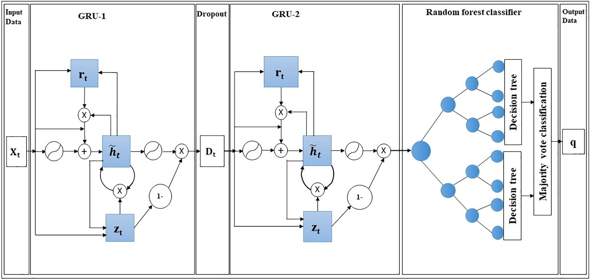
Figure 1: GRU-RF-RTC model architecture

The dropout layer between the first and second layers regulates the network and trains the weight using batch training iteration (by dropping some weights turn by turn from the first layer). This dropout technique avoids the probability of some weight dominating the other and makes all the weights trained appropriately. The dropout prevents model overfitting by randomly dropping out a fraction of the outputs from the previous layer during training and provides good performance, as explained by [68–71]. This dropout regulation helps the network to learn more robust and generalized representations. The dropout regularizing process does not change the output between the first GRU and dropout layers. The dropout’s output is an input for the second GRU layer.

The second GRU layer builds upon the features and representations learned by the first GRU layer. This layer captures additional dependencies and patterns that might have missed by the first layer. The second layer performs a deeper level of feature extractions, incorporating the learned representations from the first layer and further refining them. This layer aids the model can capture more intricate relationships and dependencies within the sequence, enabling it to learn the hierarchical data representation and generate more nuanced and accurate predictions. The presence of the second GRU layer makes the model more effective in capturing information not cached by the first GRU layer.

The output of the second layer is flattened and fed to the random forest (RF) classifier. The RF classifier determines the production process status using the features extracted by the GRU layers as input. The output of RF is a batch of (bs, n0). As a process monitoring using a binary classification task, n0 is set to be one, as mentioned in the literature as a convention [4]. If the monitoring result is closer to one, the production process is more likely to be out of control (shifted), whereas the production is in control if the result is closer to zero.

The detailed flow process chart of the proposed method is presented in Fig. 2. The data are collected from the production machines using sensors. The multivariate time series sensor data are fed into a stacked GRU network based on the specified moving window size. Then, the GRU extracts important features from these input sensor data and feed them into the RF classifier. The RF classifier performs classification and displays monitoring statistics indicating whether the process is in-control or out-of-control. This mapping of input data to a sequence of output data is performed using consecutive computations defined from Eqs. (1) to (5) above. The process is performed continuously when a new observation is added to the moving window and for every new data, the model monitor and examine whether the process is out of control or in control.

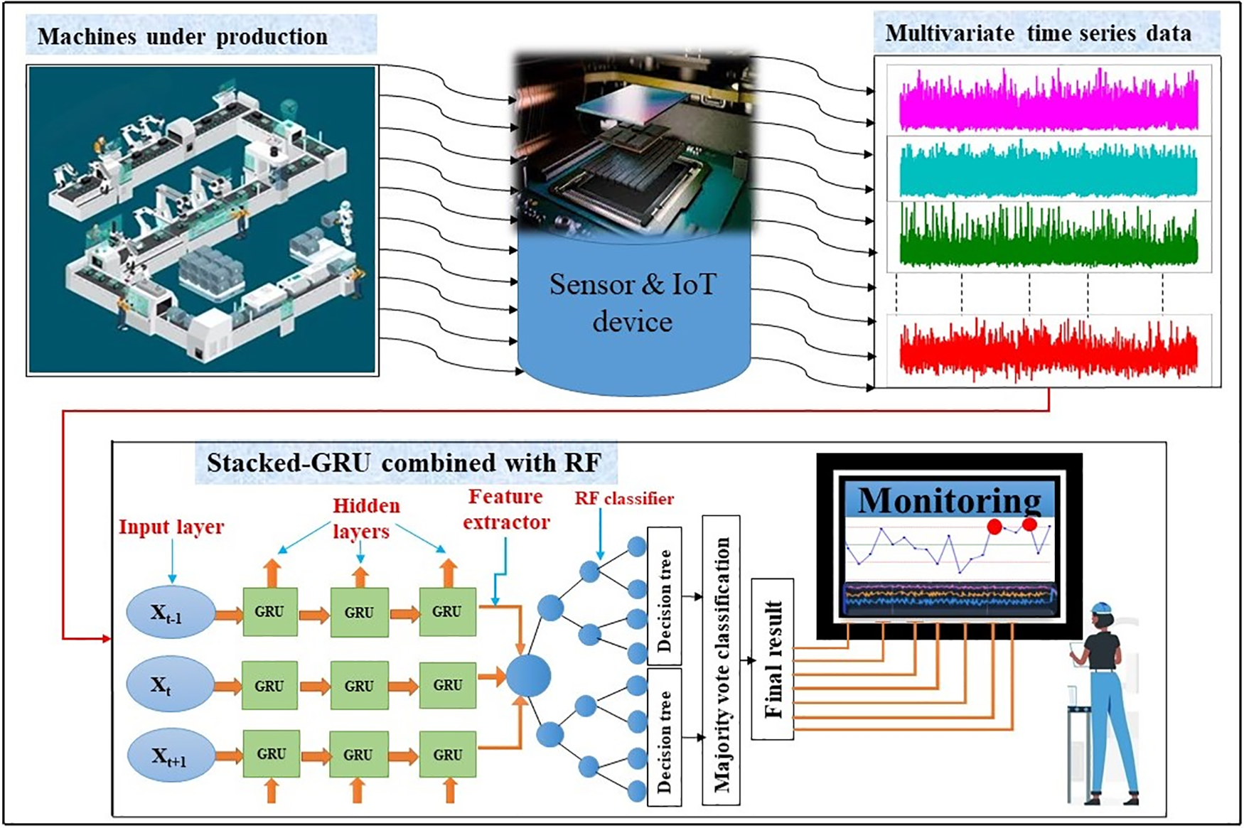
Figure 2: Illustration of flow-process chart of GRU-RF-RTC monitoring model

4  Experiments and Results

4.1 Experimental Settings

Control Limit (CL)

To classify the process as either in-control or out-of-control, a detection threshold (control limit) h is determined for each data value through consecutive simulation, reflecting the production process’s status. The control limit acts as a threshold level for the GRU-RF-RTC MPM in assessing the production status. In order to enhance the monitoring accuracy of the GRU-RF-RTC approach, a search is performed to find the optimal control limit for each problem. The control limit is crucial for achieving better detection precision for MPM [4]. The control chart releases a few false alarms when the system is in-control. However, if the process shifts to an abnormal condition (out-of-control), it surpasses the CL and generates more false alarms. As mentioned above, the RL1 is the time elapsed from the occurrence of the process shift until its detection, while the in-control run length (RL0) represents the duration until a false alarm is triggered. The model’s performance is evaluated based on the ARL1 determined from a large set of observations. A lower ARL1 value indicates better performance while maintaining a constant ARL0. The CL is determined by setting ARL0 close to 200 as mentioned in literatures [3,4,11,17].

Hyperparameter Section

The hyperparameters of the combined model (DL and ML) were determined using trial-and-error procedures without utilizing an optimization algorithm. The hyperparameters were selected using iterative procedures based on various combinations of hyperparameters and examining model performance using ARL1 metrics [72]. This iterative technique is executed continuously by adjusting the hyperparameters until the best configuration that provides minimum ARL1 values is found.

Result Comparison Procedures

This section presents performance comparison procedures using synthesis and real-world datasets in various volumes, dimensions, and distributions. The comparison was conducted in three stages, as described below. Firstly, the performance of the proposed model was compared with benchmark methods using datasets of varying volumes under normal distributions. The objective of this comparison was to evaluate the effectiveness of the proposed model across different data volumes and assess its performance relative to the benchmark methods. Secondly, the comparison was conducted based on data variety under normal distributions. This stage evaluates the proposed model’s ability to handle diverse data dimensions. By comparing the performance of the proposed model with other methods across different data varieties, we can gain insights into its strengths and weaknesses.

In addition, the proposed model was tested using a synthesis bivariate gamma distribution dataset to validate the model performance for non-normal distributions. Thirdly, the comparison was carried out using real-world datasets to validate and ensure the proposed model’s performance and applicability in real manufacturing scenarios. These datasets were collected from real-manufacturing processes and other sources encompassing normal and non-normal distribution. Testing the proposed model using real-world data enables us to assess its effectiveness and suitability for practical industrial applications. Through these consecutive comparisons, we aim to comprehensively evaluate the proposed model’s performance and the potential for real-world implementation in manufacturing settings.

To conduct the experiments, researchers utilized the evaluation framework outlined in the literature [4,17]. In addition, a bivariate gamma problem with δ = 0 to δ = 3 and real-world data: wine production [73], paper production [5], predictive maintenance [74], and MAGIC gamma Telescope [75] datasets were used to examine the performance capability of the proposed models from simple to relatively complex problems. These comparisons used the original parameters settings of RF-RTC and LSTM-RTC for each benchmarking reference data size: S0 = 1000 for RF-RTC [11] and S0 = 100,000 for LSTM-RTC [4] except for the two real-world data. Also, the reference data size for GRU-RTC and the proposed GRU-RF-RTC models are set to S0 = 100,000, which is the common data size recorded by most IoT devices in smart manufacturing [4,5].

The ARL1 is determined using Eq. (7), with N representing the replication number. In this study, a value of 1000 was chosen for N to ensure consistent results. To assess the variation of RL1, we employed the standard error denoted as SE. Statistical testing of the performance difference was conducted using a 95% confidence interval. To ensure a fair comparison, we set the control limits for each chart according to conventional standards that achieve an average in-control run-length (ARL0) of approximately 200 [11].

ARL=1N∑n=1NRLr(7)

The process shift of multivariate normal distribution is determined using Eq. (8). In these equations, μ1 and μ0 represent the mean values of the out-of-control and in-control processes, respectively, and Σ denotes the covariance matrix in a p-dimensional multivariate dataset. The process shift, denoted as δ = √5, implies that the mean values of five variables in the dataset (e.g., 50-dimensional or 100-dimensional) are shifted by one unit.

δ=(µ1−µ0)′Σ−1(µ1−µ0)(8)

The detection improvement of the proposed model is determined in terms of percentage utilizing Eq. (9). In the equation, A and B represent the best benchmark and best proposed ARL1 values, respectively. The percentage improvement shows an improvement in shift detection. This improvement (quick shift detection) reduces production interruption and the possibility of producing defective products. This quick process shift detection capability reduces waste of materials and rework costs and enhances resource optimization. These processes ensure quality control and efficiency of manufacturing systems, contributing to a more effective and competitive manufacturing environment.

Improvement(%)=A−BA∗100(9)

4.2 Result on Synthesis Data

This section compares the results obtained using different data volumes for 10- and 100-dimension and constant volumes for different data dimensions of synthesis normal distribution problems.

4.2.1 Results on Multivariate Data Volumes

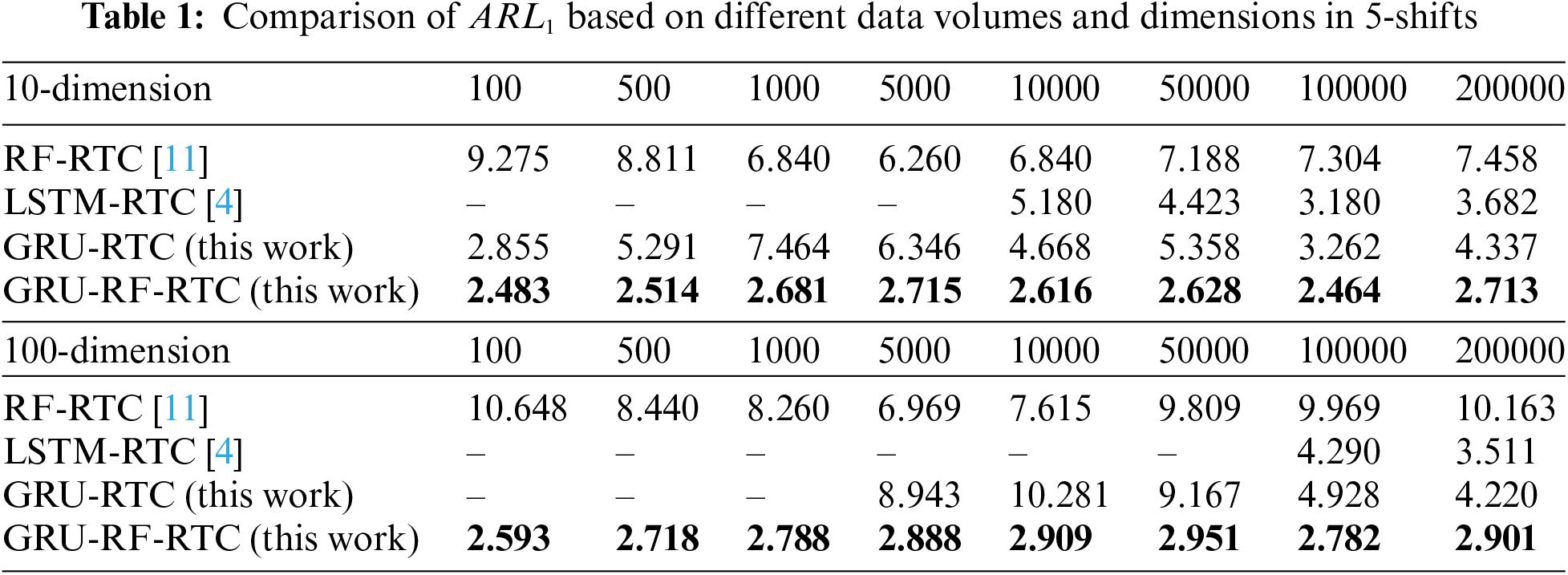
The comparison between the proposed GRU-RF-RTC model and benchmark methods is presented in Table 1. As seen from the table, the stability of the LSTM-RTC model is compromised when dealing with data volumes below 10,000 in the 10-dimensional case and below 100,000 in the 100-dimensional case. Although RF-RTC and GRU-RTC exhibit stability across most data volumes in both dimensions, they yield higher ARL1 values. Conversely, the GRU-RF-RTC model consistently performs well across different data volumes and dimensions, surpassing all benchmark models in all problem scenarios. Its exceptional performance highlights its ability to handle diverse data volumes and dimensions effectively.

4.2.2 Results on Multivariate Data Varieties

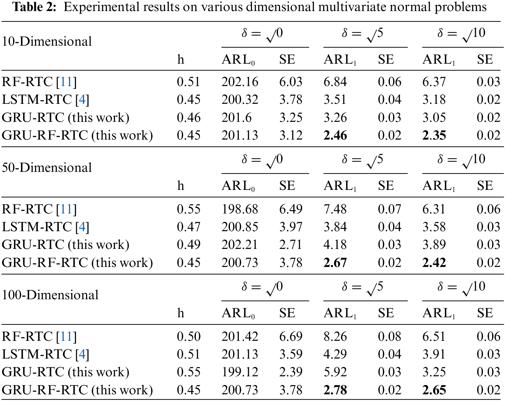
In this section, comparisons were conducted based on data variety. Table 2 presents the comparison results of the proposed and benchmark methods for different dimensions (10, 50, and 100) with shifts of 5 and 10. The results indicate a significant variation between the ARL1 values of the proposed and benchmark models, which reveal that GRU-RF-RTC outperforms benchmark methods for monitoring the manufacturing process under various dimensional problems.

4.2.3 Results on Multivariate Gamma Datasets

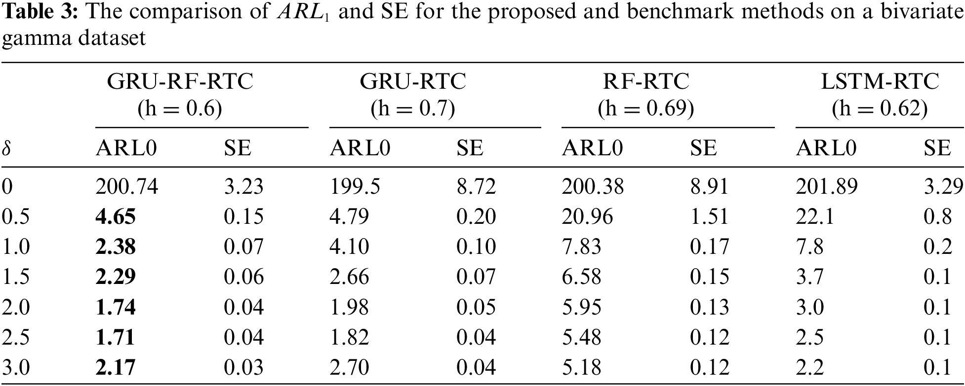
In this subsection, the performance of the proposed method on a multivariate non-normal dataset is presented. The data for in-control gamma distribution is generated with a shape parameter 1 and rate parameter 1. On the other hand, for out-of-control, the shape parameter is kept at 1, and the rate parameter is varied to simulate the mean and variance shifts. Six different shift amounts (λ = 0.5, 1, 1.5, 2, 2.5, and 3) are considered, which uniformly shift all variables. The process shift increases as the rate parameter decreases. For this, a moving window size of 10 is set. The procedure follows the same method used by [14], which was previously investigated by [17].

Table 3 compares the proposed method with the existing methods. The ARL1 and SE in the column show each model’s average run length and standard deviations, respectively. The table highlights that the GRU-RF-RTC method outperforms the benchmark method, as the boldface shows. The GRU-RF-RTC method consistently achieves lower values of ARL1 and SE for all types of process shifts. These results demonstrate that the GRU-RF-RTC model is highly effective in detecting process shifts early and significantly reduces the ARL1 value, regardless of the magnitude of the shift in the gamma distribution cases. Also, the findings indicate that the proposed GRU-RF-RTC method is not only valuable for monitoring normal distribution but also it is an excellent process monitoring model for gamma distribution cases as well.

4.3 Results on Multiple Real-World Datasets

To evaluate the performance of the proposed method, we conducted tests using both real-world normal and non-normal datasets. We utilized wine production, purple production, and predictive maintenance datasets for normal distribution cases. On the other hand, for non-normal distribution cases, we employed the Cherenkov gamma ray telescope. The findings for each case study are presented in the following section.

4.3.1 Real-World Datasets

Wine Production Datasets

The comparison of ARL1 value using the wine dataset between the proposed GRU-RF-RTC and the benchmark models is presented in this section. As studied by [76], the quality indexes of wine are converted into a binary classification. The classification is categorized as good if the index is 7 and above; else classified as bad if the index is 6 and below. The dataset has 4898 instants with 11 variables. The Z scale normalization was used to normalize the datasets.

Paper Production Dataset

The usage of chemicals, pulp fiber, and other process variables (blades, rotor speed) was recorded by sensors in paper production lines for continuous monitoring of paper breakage. The dataset consists of 18,398 data samples with 61 features. The data were normalized using Z-scale normalization. Detailed information regarding this dataset is available in [5]. From the dataset, 13,398 instances were set as the training set, while 5000 instances were used for validation. Similarly, S0 was considered reference data from the training data. The validation dataset was employed to evaluate the performances of the proposed and benchmark methods and determine the control limit.

Predictive Maintenance Datasets

A real-world predictive maintenance dataset was used to evaluate the model’s performance in detecting machine failure occurrences while the machine is working. The objective is to detect machine failures as quickly as possible, which is similar to detecting changes in the production process. The predictive maintenance dataset used in the experiments consists of 10,000 data points with 6 features. The data were normalized using z-score normalization before experimenting. The details about the dataset are available in the UCI machine learning repository [74]. First, the dataset was divided into training (7500 data instances) and validation (2500 data instances). The S0 was taken from the training dataset, and the threshold levels (CL) were determined using the validation dataset. Then, the model’s performance against the benchmark was evaluated through consecutive experiments.

Multivariate Non-Normal Datasets

A real-world data from the Cherenkov gamma ray telescope was used for evaluating the proposed GRU-RF-RTC. The data contains 19020 samples, from which 6688 hadron events and 12,332 are gamma events with 10 Hillas parameters (attributes), which are Length, Width, Size, Conc, Conc1, Asym, M3Long, M3Trans, Alpha, and Dist. The data is available publicly in the UCI machine learning repository in the name of MAGIC Gamma Telescope [75]. The study aims to classify gamma particles (signal) from the images of hadronic showers initiated by cosmic rays in the upper atmosphere background. Previously, researchers used this data in outlier detection [77,78] and process shift detection [17]. In this study, the gamma events are considered reference data, and the hadron events are a shift.

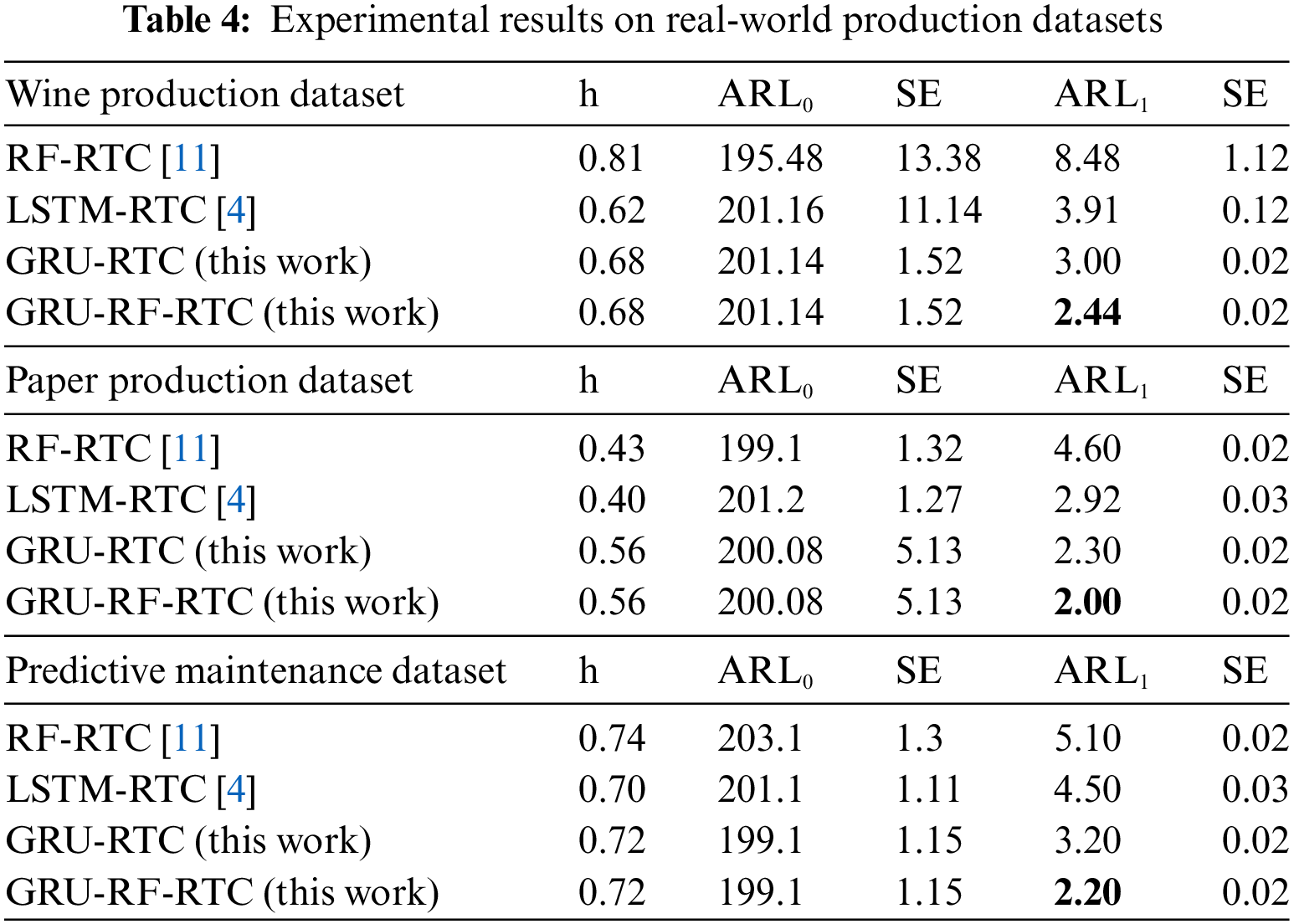
4.3.2 Results on Real-World Datasets

The summary of the analysis of the three real-world problems mentioned above (wine, paper, and predictive maintenance) is presented in Table 4. As can be seen, the proposed GRU-RF-RTC detects the process shift quicker than the benchmark methods. In predictive maintenance problem, quicker detection means it catches the machine failures as quickly as possible when it occurs. Based on this understanding, the result indicates that the GRU-RF-RTC method detects machine failure faster than the benchmark methods. This shows the proposed method is critical in monitoring the machine’s condition and manufacturing process.

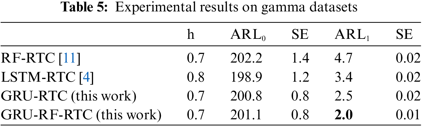
For the result of multivariate non-normal datasets, as can be seen from the normal Q-Q Fig. 3 below, the data is not the multivariate normal distribution. The experiment was conducted by taking 13,000 data from gamma events as reference data and 5000 from hadron events as a shift. Table 5 presents the detection performance of the GRU-RF-RTC against benchmarks. The results indicate that GRU-RF-RTC outperforms the benchmarks in detecting shifts. So, the proposed GRU-RF-RTC is also critical for monitoring non-normal distribution problems, which are common in manufacturing processes.

Figure 3: Normal Q-Q plots for various variables at gamma events in the MAGIC gamma telescope data

4.4 Discussion

This study compared the proposed GRU-RF-RTC model with benchmark methods, including RF-RTC, LSTM-RTC, and GRU-RTC, on synthesized MTS datasets with normal and gamma distributions. Additionally, we evaluated the model’s performance on real-world datasets, such as wine and paper production cases, a predictive maintenance problem, and the MAGIC Gamma Telescope dataset. The experimental results demonstrate that the GRU-RF-RTC model outperforms all the benchmarks in terms of quicker process shift detection as indicated by smaller ARL1 values. This superiority can be attributed to the combined effect of GRU’s capability in feature extraction and the robustness of RF in classification. In the literature, machine learning (ML) methods such as RF-RTC [11] and deep learning (DL) methods such as LSTM-RTC [4] have shown better performance in shift detection compared to traditional monitoring methods. However, previous studies have not explored the combined application of the mentioned ML and DL methods in process monitoring. This study aims to showcase the synergistic effects of RF and GRU to enhance the performance of manufacturing process monitoring methods. The results presented in Tables 1–5 demonstrate the superior performance of the GRU-RF-RTC method compared to the benchmark methods in promptly detecting process shifts from normal operating conditions. Specifically, the proposed GRU-RF-RTC method enhances the detection capability by 42.14% in normal and 43.64% in gamma distribution cases.

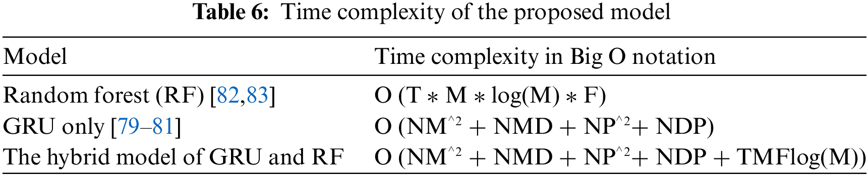
The time complexity of the proposed model is described in terms of Big-O notation. In GRU, the complexity depends on the input sequence length N, input dimension D, units in the first M, and units in the second layers P of GRU [79–81], while RF depends on the number of trees T, the number of samples in dataset M, and the number of features in dataset F [82,83]. Therefore, the time complexity of the proposed hybrid model can be approximated as the time complexity of the summation of the GRU and RF as seen in Table 6. Obviously, the proposed hybrid GRU and RF have more time complexity than GRU and RF individually. However, the proposed model achieved higher performance in terms of ARL1 and SE.

The application of DL and ML is common in manufacturing. Also, the GRU-RF-RTC is compatible with standard manufacturing software and hardware systems because various software has been developed in the past and applied in manufacturing systems. For example, a Manufacturing executive system (MES) is one of the software integrated with DL and ML in a manufacturing system [84]. In this, ML is integrated into multi-agent MES for anomaly detection. In addition, various graphical user interfaces (GUI) [85] are suitable for interacting with practitioners with various DL and ML. This GUI can simplify data input, model configuration, and result interpretation. For instance, WEKA and Orange are typical GUI tools that provide an integrated environment with an interactive interface used for data mining and visualizations [86]. Also, the proposed model used automated data preprocessing, such as data cleaning, feature extraction, and scaling, which avoids manual work [86]. These properties make the proposed model user-friendly.

DL and ML played significant results in manufacturing applications. However, they encounter challenges when applied in real manufacturing scenarios. The model required powerful computational resources such as hardware, regular model updating, continuous training to acquire the required knowledge regarding data analysis, availability of data quality, and access and feeding real-time data into the model with the compatibility of typical data acquisition systems [87].

5  Conclusion

This research proposed a new MPM method combining GRU and RF to monitor and detect process shifts quickly. The proposed method leverages the strengths of both GRU and RF. GRU is utilized for feature extraction, and the extracted features are then fed to RF for classification. GRU is highly effective in extracting features, while RF is a robust and interpretable algorithm commonly used for classification tasks. By combining GRU and RF, the proposed model enables automatic feature extraction from small and large datasets without overfitting, resulting in accurate classification and enhanced robustness in detecting changes in the production process.

The robustness of the monitoring model is essential for maintaining the system’s reliability. The proposed method was tested using multivariate synthesis and real-world problems with normal and non-normal data distributions. The proposed model demonstrates quicker process shift detection with smaller ARL1 values than existing methods. The GRU-RF-RTC method improves detection time and can be applied to monitor datasets of any size, addressing a research gap in previous work. Significantly, the combination of GRU and RF enhances the model’s robustness in monitoring and quick detection and enables it to handle datasets of any distribution, variety and size. The results indicate that the proposed GRU-RF-RTC model enhances shift detection by 42.14% in normal distribution problems and 43.64% in gamma distribution problems.

Based on the experimental result, researchers showcased the effectiveness of the GRU-RF-RTC in multivariate process monitoring under normal and gamma distribution cases. Further study can be conducted to investigate the performance of the proposed model in other types of data distribution, such as Poisson and t-distribution. Although the proposed method is effective in multivariate process monitoring, a follow-up study can be extended to demonstrate its detection capability on other process monitoring methods, such as the exponentially weighted moving average (EWMA). Additionally, exploring and validating the combination of other deep learning and machine learning classifiers for MPM applications would be an interesting avenue for research. Moreover, exploring the potential of process monitoring using the image-based encoding of time series data is worthwhile. The trade-off of model accuracy and complexity can be studied for algorithm efficiency. Last but not least, extending the application of this model to other domains would be a valuable extension of the research.

Acknowledgement: Not applicable.

Funding Statement: We appreciate the financial support from the National Science and Technology Council of Taiwan (Contract Nos. 111-2221 E-011081 and 111-2622-E-011019) and the support from Intelligent Manufacturing Innovation Center (IMIC), National Taiwan University of Science and Technology (NTUST), Taipei, Taiwan, which is a Featured Areas Research Center in Higher Education Sprout Project of Ministry of Education (MOE), Taiwan (since 2023) was appreciated. We also thank Wang Jhan Yang Charitable Trust Fund (Contract No. WJY 2020-HR-01) for its financial support.

Author Contributions: Study conception and design: C. -L. Yang, A. A. Yilma, B. H. Woldegiorgis; data collection: A. A. Yilma, Tampubolon, H., Sutrisno, H.; analysis and interpretation of results: C. -L. Yang, A. A. Yilma, Tampubolon, H., Sutrisno H.; investigation: B. H. Woldegiorgis, Tampubolon, H., Sutrisno H.; manuscript preparation: C. -L. Yang, A. A. Yilma, B. H. Woldegiorgis. All authors reviewed the results and approved the final version of the manuscript.

Availability of Data and Materials: Not applicable.

Conflicts of Interest: The authors declare that they have no conflict of interest to report regarding the present study.

References

1. F. Tao and Q. Qi, “New IT driven service-oriented smart manufacturing: Framework and characteristics,” IEEE Trans. Syst., Man, Cybernet.: Syst., vol. 49, no. 1, pp. 81–91, 2017. [Google Scholar]

2. P. Lade, R. Ghosh, and S. Srinivasan, “Manufacturing analytics and industrial internet of things,” IEEE Intell. Syst., vol. 32, no. 3, pp. 74–79, 2017. [Google Scholar]

3. S. He, W. Jiang, and H. Deng, “A distance-based control chart for monitoring multivariate processes using support vector machines,” Ann. Oper. Res., vol. 263, pp. 191–207, 2018. [Google Scholar]

4. C. L. Yang and H. Sutrisno, “Reducing response delay in multivariate process monitoring by a stacked long-short term memory network and real-time contrasts,” Comput. Ind. Eng., vol. 153, pp. 107052, 2021. [Google Scholar]

5. C. Ranjan, M. Reddy, M. Mustonen, K. Paynabar, and K. Pourak, “Dataset: Rare event classification in multivariate time series,” arXiv preprint arXiv:1809.10717, 2018. [Google Scholar]

6. A. Khodabakhsh, I. Ari̇, M. Bakír, and A. O. Ercan, “Multivariate sensor data analysis for oil refineries and multi-mode identification of system behavior in real-time,” IEEE Access., vol. 6, pp. 64389–64405, 2018. [Google Scholar]

7. Z. Ye, C. Liu, W. Tian, and C. Kan, “In-situ point cloud fusion for layer-wise monitoring of additive manufacturing,” J. Manuf. Syst., vol. 61, pp. 210–222, 2021. [Google Scholar]

8. C. F. Chien, W. T. Hung, C. W. Pan, and T. H. V. Nguyen, “Decision-based virtual metrology for advanced process control to empower smart production and an empirical study for semiconductor manufacturing,” Comput. Ind. Eng., vol. 169, pp. 108245, 2022. [Google Scholar]

9. T. Biegel, N. Jourdan, C. Hernandez, A. Cviko, and J. Metternich, “Deep learning for multivariate statistical in-process control in discrete manufacturing: A case study in a sheet metal forming process,” in Proc. CIRP, vol. 107, pp. 422–427, 2022. [Google Scholar]

10. J. C. Kabugo, S. L. Jämsä-Jounela, R. Schiemann, and C. Binder, “Process monitoring platform based on industry 4.0 tools: A waste-to-energy plant case study,” in 2019 4th Conf. Control Fault Tolerant Syst. (SysTol), Casablanca, Morocco, 2019, pp. 264–269. [Google Scholar]

11. H. Deng, G. Runger, and E. Tuv, “System monitoring with real-time contrasts,” J. Qual. Technol., vol. 44, no. 1, pp. 9–27, 2012. [Google Scholar]

12. T. Haanchumpol, P. Sudasna-na-Ayudthya, and C. Singhtaun, “Modern multivariate control chart using spatial signed rank for non-normal process,” Eng. Sci. Technol. Int. J., vol. 23, no. 4, pp. 859–869, 2020. [Google Scholar]

13. S. Sikder, S. C. Panja, and I. Mukherjee, “An integrated approach for multivariate statistical process control using Mahalanobis-Taguchi system and Andrews function,” Int. J. Qual. Reliab. Manag., vol. 34, no. 8, pp. 1186–1208, 2017. [Google Scholar]

14. F. K. Wang, B. Bizuneh, and X. B. Cheng, “One-sided control chart based on support vector machines with differential evolution algorithm,” Qual. Reliab. Eng. Int., vol. 35, no. 6, pp. 1634–1645, 2019. [Google Scholar]

15. M. Zhang, J. Guo, X. Li, and R. Jin, “Data-driven anomaly detection approach for time-series streaming data,” Sens., vol. 20, no. 19, pp. 5646, 2020. [Google Scholar]

16. A. Sahar and D. Han, “An LSTM-based indoor positioning method using Wi-Fi signals,” in Proc. 2nd Int. Conf. Vis., Image Signal Process., Las Vegas, NV, USA, 2018, pp. 1–5. [Google Scholar]

17. S. Jang, S. H. Park, and J. -G. Baek, “Real-time contrasts control chart using random forests with weighted voting,” Expert Syst. Appl., vol. 71, pp. 358–369, 2017. [Google Scholar]

18. L. Breiman, “Random forests,” Mach. Learn., vol. 45, pp. 5–32, 2001. [Google Scholar]

19. L. Breiman, Manual on Setting Up, Using, and Understanding Random Forests v3.1, Berkeley, CA, USA: Statistics Department University of California, 2002, vol. 1, pp. 3–42. [Google Scholar]

20. T. Wuest, D. Weimer, C. Irgens, and K. D. Thoben, “Machine learning in manufacturing: Advantages, challenges, and applications,” Prod. Manuf. Res., vol. 4, no. 1, pp. 23–45, 2016. [Google Scholar]

21. R. Rai, M. K. Tiwari, D. Ivanov, and A. Dolgui, “Machine learning in manufacturing and industry 4.0 applications,” Int. J. Prod. Res., vol. 59, no. 16, pp. 4773–4778, 2021. [Google Scholar]

22. A. A. Nuhu, Q. Zeeshan, B. Safaei, and M. A. Shahzad, “Machine learning-based techniques for fault diagnosis in the semiconductor manufacturing process: A comparative study,” J. Supercomput., vol. 79, no. 2, pp. 2031–2081, 2023. [Google Scholar]

23. J. Sharma, M. L. Mittal, and G. Soni, “Condition-based maintenance using machine learning and role of interpretability: A review,” Int. J. Syst. Assur. Eng. Manag., vol. 20, pp. 1–16, 2022. [Google Scholar]

24. M. Ismail, N. A. Mostafa, and A. El-assal, “Quality monitoring in multistage manufacturing systems by using machine learning techniques,” J. Intell. Manuf., vol. 33, no. 8, pp. 2471–2486, 2022. [Google Scholar]

25. J. M. Barrera, A. Reina, A. Mate, and J. C. Trujillo, “Fault detection and diagnosis for industrial processes based on clustering and autoencoders: A case of gas turbines,” Int. J. Mach. Learn. Cyb., vol. 13, no. 10, pp. 3113–3129, 2022. [Google Scholar]

26. H. Zermane and A. Drardja, “Development of an efficient cement production monitoring system based on the improved random forest algorithm,” Int. J. Adv. Manuf. Technol., vol. 120, no. 3–4, pp. 1853–1866, 2022. [Google Scholar]

27. M. K. Msakni, A. Risan, and P. Schütz, “Using machine learning prediction models for quality control: A case study from the automotive industry,” Comput. Manag. Sci., vol. 20, no. 1, pp. 14, 2023. [Google Scholar] [PubMed]

28. L. Bertoli, F. Caltanissetta, and B. M. Colosimo, “In-situ quality monitoring of extrusion-based additive manufacturing via random forests and clustering,” in 2021 IEEE 17th Int. Conf. Autom. Sci. Eng. (CASE), Lyon, France, 2021, pp. 2057–2062. [Google Scholar]

29. P. Mohammadi and Z. J. Wang, “Machine learning for quality prediction in abrasion-resistant material manufacturing process,” in 2016 IEEE Canadian Conf. Electr. Comput Eng. (CCECE), 2016, pp. 1–4. [Google Scholar]

30. A. Yoo, Y. Oh, H. Park, N. Kim, D. Kim and Y. Kim, “A product quality monitoring framework using SVM-based production data analysis in online shop floor controls,” in Proc. of IIE Annual Conf., Ulsan, South Korea, 2013, pp. 3255– 3262. [Google Scholar]

31. B. M. Mun, M. Lim, and S. J. Bae, “Condition monitoring scheme via one-class support vector machine and multivariate control charts,” J. Mech. Sci. Technol., vol. 34, pp. 3937–3944, 2020. [Google Scholar]

32. H. Fahad and G. J. Asmaa, “Using support vector machine to determine the limits of multivariate control charts,” J. Phys.: Conf. Ser., vol. 1897, pp. 012009, 2021. [Google Scholar]

33. Y. Oh, M. Busogi, K. Ransikarbum, D. Shin, D. Kwon and N. Kim, “Real-time quality monitoring and control system using an integrated cost effective support vector machine,” J. Mech. Sci. Technol., vol. 33, pp. 6009–6020, 2019. [Google Scholar]

34. T. L. Tseng, K. R. Aleti, Z. Hu, and Y. Kwon, “E-quality control: A support vector machines approach,” J. Comput. Des. Eng., vol. 3, no. 2, pp. 91–101, 2016. [Google Scholar]

35. Q. Wei, W. Huang, W. Jiang, and W. Zhao, “Real-time process monitoring using kernel distances,” Int. J. Prod. Res., vol. 54, no. 21, pp. 6563–6578, 2016. [Google Scholar]

36. K. S. Shin, I. S. Lee, and J. G. Baek, “An improved real-time contrasts control chart using novelty detection and variable importance,” Appl. Sci., vol. 9, no. 1, pp. 173, 2019. [Google Scholar]

37. J. Wang, Y. Ma, L. Zhang, R. X. Gao, and D. Wu, “Deep learning for smart manufacturing: Methods and applications,” J. Manuf. Syst., vol. 48, pp. 144–156, 2018. [Google Scholar]

38. E. Rama-Maneiro, J. Vidal, and M. Lama, “Deep learning for predictive business process monitoring: Review and benchmark,” IEEE Trans. Serv. Comput., vol. 16, no. 1, pp. 739–756, 2021. [Google Scholar]

39. X. Yan, Y. Liu, Y. Xu, and M. Jia, “Multistep forecasting for diurnal wind speed based on hybrid deep learning model with improved singular spectrum decomposition,” Energ. Convers. Manage., vol. 225, pp. 113456, 2020. [Google Scholar]

40. Q. Chen, Q. Xie, Q. Yuan, H. Huang, and Y. Li, “Research on a real-time monitoring method for the wear state of a tool based on a convolutional bidirectional LSTM model,” Symmetry, vol. 11, no. 10, pp. 1233, 2019. [Google Scholar]

41. G. Zhang, H. Xiao, J. Jiang, Q. Liu, Y. Liu and L. Wang, “A multi-index generative adversarial network for tool wear detection with imbalanced data,” Complexity, vol. 2020, pp. 1–10, 2020. [Google Scholar]

42. M. Shah, H. Borade, V. Sanghavi, A. Purohit, V. Wankhede and V. Vakharia, “Enhancing tool wear prediction accuracy using walsh-hadamard transform, DCGAN and dragonfly algorithm-based feature selection,” Sens., vol. 23, no. 8, pp. 3833, 2023. [Google Scholar]

43. K. Li, M. Chen, Y. Lin, Z. Li, X. Jia and B. Li, “A novel adversarial domain adaptation transfer learning method for tool wear state prediction,” Knowl.-Based Syst., vol. 254, pp. 109537, 2022. [Google Scholar]

44. Z. Chen, S. Deng, X. Chen, C. Li, R. V. Sanchez and H. Qin, “Deep neural networks-based rolling bearing fault diagnosis,” Microelectron. Reliab., vol. 75, pp. 327–333, 2017. [Google Scholar]

45. X. Yan, D. She, and Y. Xu, “Deep order-wavelet convolutional variational autoencoder for fault identification of rolling bearing under fluctuating speed conditions,” Expert Syst. Appl., vol. 216, pp. 119479, 2023. [Google Scholar]

46. P. Tamilselvan and P. Wang, “Failure diagnosis using deep belief learning based health state classification,” Reliab. Eng. Syst. Safe., vol. 115, pp. 124–135, 2013. [Google Scholar]

47. X. Yan, D. She, Y. Xu, and M. Jia, “Deep regularized variational autoencoder for intelligent fault diagnosis of rotor-bearing system within entire life-cycle process,” Knowl.-Based Syst., vol. 226, pp. 107142, 2021. [Google Scholar]

48. X. Yan, Y. Liu, and M. Jia, “Multiscale cascading deep belief network for fault identification of rotating machinery under various working conditions,” Knowl.-Based Syst., vol. 193, pp. 105484, 2020. [Google Scholar]

49. J. Lee, Y. C. Lee, and J. T. Kim, “Fault detection based on one-class deep learning for manufacturing applications limited to an imbalanced database,” J. Manuf. Syst., vol. 57, pp. 357–366, 2020. [Google Scholar]

50. D. Fuqua and T. Razzaghi, “A cost-sensitive convolution neural network learning for control chart pattern recognition,” Expert. Syst. Appl., vol. 150, pp. 113275, 2020. [Google Scholar]

51. X. Li, S. Siahpour, J. Lee, Y. Wang, and J. Shi, “Deep learning-based intelligent process monitoring of directed energy deposition in additive manufacturing with thermal images,” Procedia Manuf., vol. 48, pp. 643–649, 2020. [Google Scholar]

52. H. Ko, J. Kim, Y. Lu, D. Shin, Z. Yang and Y. Oh, “Spatial-temporal modeling using deep learning for real-time monitoring of additive manufacturing,” in Int. Des. Eng. Techn. Conf. Comput. Inf. Eng. Conf., St. Louis, Missouri, USA, 2022, pp. V002T02A019. [Google Scholar]

53. X. Yan, Y. Liu, and M. Jia, “Health condition identification for rolling bearing using a multi-domain indicator-based optimized stacked denoising autoencoder,” Struct. Health Monit., vol. 19, no. 5, pp. 1602–1626, 2020. [Google Scholar]

54. K. Cho et al., “Learning phrase representations using RNN encoder-decoder for statistical machine translation,” arXiv preprint arXiv:1406.1078, 2014. [Google Scholar]

55. J. Wang, J. Yan, C. Li, R. X. Gao, and R. Zhao, “Deep heterogeneous GRU model for predictive analytics in smart manufacturing: Application to tool wear prediction,” Comput. Ind., vol. 111, pp. 1–14, 2019. [Google Scholar]

56. Y. Han, Z. Du, Z. Geng, Y. Wang, F. Xie and K. Chen, “Production prediction model of complex industrial processes based on GRU neural network,” in 2020 Chinese Automation Congress (CAC), 2020,pp. 1102–1106. [Google Scholar]

57. C. Wang, W. Du, Z. Zhu, and Z. Yue, “The real-time big data processing method based on LSTM or GRU for the smart job shop production process,” J. Algorithms Comput. Technol., vol. 14, pp. 1748302620962390, 2020. [Google Scholar]

58. B. C. Mateus, M. Mendes, J. T. Farinha, A. M. Cardoso, R. Assis and H. Soltanali, “Improved GRU prediction of paper pulp press variables using different pre-processing methods,” Prod. Manuf. Res., vol. 11, no. 1, pp. 2155263, 2023. [Google Scholar]

59. R. Fu, Z. Zhang, and L. Li, “Using LSTM and GRU neural network methods for traffic flow prediction,” in 2016 31st Youth Acad. Ann. Conf. Chinese Assoc. Autom. (YAC), Wuhan, China, 2016, pp. 324–328. [Google Scholar]

60. P. Qashqai, R. Zgheib, and K. Al-Haddad, “GRU and LSTM comparison for black-box modeling of power electronic converters,” in IECON 2021-47th Ann. Conf. IEEE Indust. Electr. Soc., Toronto, ON, Canada, 2021, pp. 1–5. [Google Scholar]

61. P. Ambadekar and C. Choudhari, “CNN based tool monitoring system to predict life of cutting tool,” SN. Appl. Sci., vol. 2, pp. 1–11, 2020. [Google Scholar]

62. R. Kou, S. W. Lian, N. Xie, B. E. Lu, and X. M. Liu, “Image-based tool condition monitoring based on convolution neural network in turning process,” Int. J. Adv. Manuf. Technol., vol. 119, pp. 3279–3291, 2022. [Google Scholar]

63. F. Jansen, M. Holenderski, T. Ozcelebi, P. Dam, and B. Tijsma, “Predicting machine failures from industrial time series data,” in 2018 5th Int. Conf Contr., Decis. Inf. Technol. (CoDIT), Thessaloniki, Greece, 2018, pp. 1091–1096. [Google Scholar]

64. C. W. Zhou and J. Jing, “Research on tool wear monitoring based on GRU-CNN,” in 2021 6th Int. Conf. Intell.nt Comput. Signal Process. (ICSP), Xi’an, China, 2021, pp. 729–733. [Google Scholar]

65. H. Widiputra, A. Mailangkay, and E. Gautama, “Multivariate CNN-LSTM model for multiple parallel financial time-series prediction,” Complexity, vol. 2021, pp. 1–14, 2021. [Google Scholar]

66. K. A. Althelaya, E. -S. M. El-Alfy, and S. Mohammed, “Stock market forecast using multivariate analysis with bidirectional and stacked (LSTM, GRU),” in 2018 21st Saudi Comput. Soc. Nat. Comput. Conf. (NCC), Riyadh, Saudi Arabia, 2018, pp. 1–7. [Google Scholar]

67. F. Pan et al., “Stacked-GRU based power system transient stability assessment method,” Alg., vol. 11, no. 8, pp. 121, 2018. [Google Scholar]

68. N. Srivastava, G. Hinton, A. Krizhevsky, I. Sutskever, and R. Salakhutdinov, “Dropout: A simple way to prevent neural networks from overfitting,” J. Mach. Learn. Res., vol. 15, no. 1, pp. 1929–1958, 2014. [Google Scholar]

69. X. Shen, X. Tian, T. Liu, F. Xu, and D. Tao, “Continuous dropout,” IEEE Trans. Neur. Net. Lear., vol. 29, no. 9, pp. 3926–3937, 2017. [Google Scholar]

70. G. Cheng, V. Peddinti, D. Povey, V. Manohar, S. Khudanpur and Y. Yan, “An exploration of dropout with LSTMs,” in Interspeech, 2017, pp. 1586–1590. [Google Scholar]

71. A. Labach, H. Salehinejad, and S. Valaee, “Survey of dropout methods for deep neural networks,” arXiv preprint arXiv:1904.13310, 2019. [Google Scholar]

72. L. Yang and A. Shami, “On hyperparameter optimization of machine learning algorithms: Theory and practice,” Neurocomput., vol. 415, pp. 295–316, 2020. [Google Scholar]

73. P. Cortez, A. Cerdeira, F. Almeida, T. Matos, and J. Reis, “Modeling wine preferences by data mining from physicochemical properties,” Decis. Support. Syst., vol. 47, no. 4, pp. 547–553, 2009. [Google Scholar]

74. AI4I, “Predictive maintenance dataset. (2020). UCI machine learning repository,” 2020. doi: 10.24432/C5HS5C. [Google Scholar] [CrossRef]

75. R. Bock, “MAGIC gamma telescope. UCI machine learning repository,” 2007. doi: 10.24432/C52C8B. [Google Scholar] [CrossRef]

76. C. Zou, W. Jiang, and F. Tsung, “A LASSO-based diagnostic framework for multivariate statistical process control,” Technometr., vol. 53, no. 3, pp. 297–309, 2011. [Google Scholar]

77. J. Liu and H. Deng, “Outlier detection on uncertain data based on local information,” Knowl.-Based Syst., vol. 51, pp. 60–71, 2013. [Google Scholar]

78. X. Ru, Z. Liu, Z. Huang, and W. Jiang, “Normalized residual-based constant false-alarm rate outlier detection,” Pattern. Recogn. Lett., vol. 69, pp. 1–7, 2016. [Google Scholar]

79. M. Rotman and L. Wolf, “Shuffling recurrent neural networks,” in Proc. AAAI Conf. Artif. Intell., 2021, pp. 9428–9435. [Google Scholar]

80. D. Alqahtani, “Leveraging sparse auto-encoding and dynamic learning rate for efficient cloud workloads prediction,” IEEE Access, vol. 11, pp. 64586–64599, 2023. [Google Scholar]

81. M. C. Lee, “Research on the feasibility of applying GRU and attention mechanism combined with technical indicators in stock trading strategies,” Appl. Sci., vol. 12, no. 3, pp. 1007, 2022. [Google Scholar]

82. K. Hassine, A. Erbad, and R. Hamila, “Important complexity reduction of random forest in multi-classification problem,” in 2019 15th Int. Wirel. Commun. Mobile Comput. Conf. (IWCMC), Tangier, Morocco, 2019, pp. 226–231. [Google Scholar]

83. L. Štěpánek, F. Habarta, I. Malá, and L. Marek, “A random forest-based approach for survival curves comparison: Principles, computational aspects, and asymptotic time complexity analysis,” in 2021 16th Conf. Comput. Sci. Intell. Syst. (FedCSIS), Sofia, Bulgaria, 2021, pp. 301–311. [Google Scholar]

84. S. Mantravadi, L. Chen, and C. Møller, “Multi-agent manufacturing execution system (MESConcept, architecture & ML algorithm for a smart factory case,” in 21st Int. Conf. Enterp. Inf. Syst., 2019, pp. 477–482. [Google Scholar]

85. S. Malik, M. T. Saeed, M. J. Zia, S. Rasool, L. A. Khan and M. I. Ahmed, “Reimagining application user interface (UI) design using deep learning methods: Challenges and opportunities,” arXiv preprint arXiv:2303.13055, 2023. [Google Scholar]

86. G. Ogunleye, S. Fashoto, C. Daramola, L. Ogundele, and T. Ojewumi, “Development of a simple graphical interface based software for machine learning and data visualization,” Int. J. Rec. Technol. Eng., vol. 8, no. 2, pp. 3770–3777, 2019. [Google Scholar]

87. R. Malhan and S. K. Gupta, “The role of deep learning in manufacturing applications: Challenges and opportunities,” J. Comput. Inf. Sci. Eng., vol. 23, no. 6, pp. 060816, 2023. [Google Scholar]