SC-Net: A New U-Net Network for Hippocampus Segmentation

1  Introduction

Alzheimer’s disease (AD) [1] is a brain neurodegenerative disease that cannot be reversed and typically affects people over 60. Cognitive decline, diminished capacity for self-care, mental symptoms, and behavioral disturbances are the primary signs. One of the first areas of a brain to show the pathological effects of AD is hippocampus [2], whose atrophied volume and shape will change depending on the stage of disease. There is currently no medicine that can cure the disease, but environment-assisted treatment can be used to slow down the disease stage by monitoring hippocampus morphovolume. As a result, the significance of effective and precise hippocampal structure segmentation is revealed in medical field.

Non-invasive imaging methods like magnetic resonance imaging (MRI) [3] are frequently utilized for disease detection, diagnosis, and treatment monitoring. Brain MRI images allow us to see internal brain structures like hippocampus and amygdala, and use imaging to make medical diagnoses. In the beginning, it took a lot of time and effort to manually segment and label hippocampus. As a result, an effective automatic segmentation of hippocampus is important for Alzheimer’s disease diagnosis and treatment. In brain MRI images, hippocampus has low contrast with the surrounding tissues and is difficult to distinguish due to small size and blurred edges. The task of segmenting MRI images of hippocampal structures has so far remained challenging.

Medical image segmentation [4] is a process of separating an area that we are interested in a medical image in order to make the changes in the anatomy or pathological structure in the image easier to see. This can effectively increase the efficiency and accuracy of diagnosis, contribute to computer-aided diagnosis, and help with smart medical treatment. The majority of the early medical image segmentation was based on various features like shape, texture, and grayscale, dividing similar regions into one category and distinct regions into another to accomplish a segmentation goal. The threshold, edge, and region equal division method are the foundations of most common methods. Numerous new methods for segmenting hippocampal structure from brain MRI have emerged in recent years as the field of artificial intelligence continues to advance. Among them, as a hot area of research, deep learning with dozens of algorithms that are suitable for various tasks and cover almost all aspects of image processing, particularly segmentation, with excellent results.

Safavian et al. [5] used a combination of LAC (location-based active contour) and SBGFRLS (selective binary and Gaussian filtering regularization level set), which used a novel level set method to implement hippocampus segmentation. Compared to Freesurfer [6], the newly proposed algorithm is more comparable to harmony hippocampus protocol (HarP) in terms of Dice segmentation accuracy. This approach has the advantage of avoiding a large database, but image preprocessing necessitates complex tasks like intensity correction and skull stripping. Liu et al. [7] utilized the fundamental framework of a convolutional neural network (CNN). They built a multi-task deep CNN model using a similar network structure, and segmented a three-dimensional density-connected convolutional network (3D), inspired by the V-Net model [8] (DenseNet), which uses the segmentation results’ features for classification and learns them. On ADNI dataset, the method achieves segmentation accuracy of 0.87 dice. However, on the HarP dataset, it achieves segmentation accuracy of 0.867 dice. Zhang et al. [9], using 3D U-Net, created a 3D U-Net cascade segmentation framework and added a cascade structure to overcome low accuracy of small target segmentation due to the hippocampus’s small size and weak boundaries. However, it needs to use CT-MRI images at the same time to obtain better segmentation results. Hosny et al. [10] proposed a multi-threshold technique for medical image segmentation, which uses both the novel c Coronavirus Optimization Algorithm (COVIDOA) and Harris Hawks Optimization Algorithm (HHOA). The entropy of Otsu and Kapur act as a fifitness functions to find the optimal threshold values to combine the two algorithms. The method was tested on 2D and 3D medical images, including MRI, CT, and X-ray images, and ultimately demonstrated superiority in multiple evaluation indicators. In 2022, a new golden jackal optimization (GJO) algorithm was proposed [11], using an OBL-based enhanced IGJO for color image segmentation to solve the multi-level threshold image segmentation problem. This method uses Ostu as the objective function of the skin cancer segmentation method, and the proposed IGJO algorithm outperforms all other algorithms in PSNR, SSIM, FSIM, and MSE segmentation indicators compared with multiple meta-heuristic methods. This method is also suitable for a variety of image problems such as visualization, computer vision, and image classification.

Since hippocampus is a part of the brain’s gray matter structure, MRI image lacks contrast, has a small volume, and its edge outline is blurry, hippocampus is difficult to accurately be segment. In addition, segmenting will be hindered by additional structures nearby the hippocampal structure, such as amygdala. Despite the fact that some existing segmentation techniques like FCN, U-Net, CNN, etc. can segment hippocampus from brain MRI, they still have to be adjusted for specific issue to obtain the best effect. To lessen the impact of irrelevant background on segmentation, some existing hippocampus segmentation methods typically require extensive preprocessing of images, such as removing skull, pre-cutting, and other operations. However, these operations will also ignore that the relative positions of various brain structures have an impact on the hippocampus’s location. At the same time, there is still room for improvement in the hippocampus’s segmentation accuracy at subtle edges. In this paper, we develop a SC-Net model based on classic U-Net, which introduces a portion of the skip-connection during the downsampling process, and makes use of edge combination loss function to improve hippocampus position features. The proposed network uses entire MRI images as a training sample, not some cropped images. The findings demonstrate that the proposed approach is capable of efficient learning and high-precision segmentation with fewer training samples, achieving a higher average segmentation level than other methods. The main contributions of SC-Net are summarized as follows:

•   Skip connections are introduced into convolution modules in the downsampling process to encoder or decoder. More features are preserved during the convolution process and strengthen the position features of hippocampus structure.

•   An end-to-end input and output model is designed to simplify the preprocessing, and preserves the influence of other brain structures’ relative positions on the hippocampus structure by using the entire brain MRI image.

•   To address the issue of hippocampus’s foreground ratio, a brand-new combination loss function is proposed, which combines Dice Loss between the segmented image’s edge contour map and the label mask with Focal Loss between the segmented image and the label mask. It can effectively eliminate background mis-segmentation interference.

The remainder of this paper is as follows. Section 2 discusses the related work. Section 3 describes the proposed model in detail. Experimental results and analysis are in Section 4. The conclusions are in Section 5.

2  Related Work

The fully convolutional network (FCN) proposed by Long et al. [12] pioneered semantic segmentation. The convolutional layer is used to replace the fully connected layer in the classification network VGG16 [13], and some spatial information of feature map is preserved to achieve pixel-level classification. Then FCN uses deconvolution and fusion feature map to restore an image, providing classification result of each pixel through the soft-max function. Since the previous fully-connected layers with dense connections are replaced by locally connected and weight-shared convolutional layers, FCN greatly reduces the number of parameters to be trained, and compared with previous methods, the performance on each test set is significantly improved.

In 2015, a version of FCN called U-Net [14] was proposed. Because of its straightforward frame structure, high accuracy, and adaptability to a variety of application scenarios, it has found widespread use in medical imaging. U-Net creates an encoder-decoder structure for semantic segmentation using the concept of FCN deconvolution to restore image size and features. By extracting feature information at each layer, the encoder reduces the spatial dimension, and the decoder gradually restores the target details and spatial dimension in accordance with the feature information.

The structure of U-Net is shown in Fig. 1. With the central axis of the U-shaped structure as the boundary, the left side of the network performs feature extraction through convolution. As the number of layers deepens, the number of channels of an image gradually increases. This part is also known as the downsampling part. The feature fusion is performed on the right side of the network, and the number of channels is continuously reduced and restored during this process, which is called the upsampling part. The overall network is an encoder-decoder structure. In order to compensate for the loss of part of information in the process of pooling and convolution during feature extraction, the encoding layer information with the same number of corresponding channels in the encoder is also added in the decoding process, which can effectively reduce feature loss.

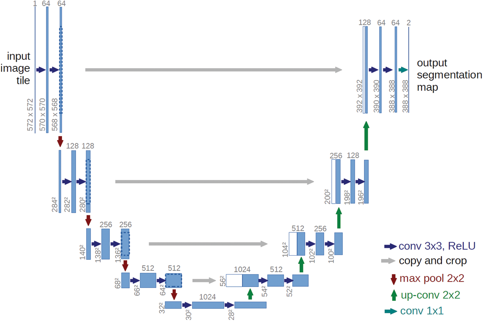
Figure 1: U-Net structure

The semantic information of medical images is relatively immobilized. Taking brain MRI images as an example, the brain tissue structure is relatively fixed, and the brain tissue will also be affected by other structures. All features are important for segmentation of targets. The use of U-Net can save low-level position features and high-level semantic features, so it has been widely used in the field of medical segmentation. At the same time, because of its lightweight construction, U-Net is easy to modify and implement. So it can be adjusted according to different segmentation tasks, provideing convenience for practical applications.

Li et al. [15] proposed a attention nested U-Net (ANU-Net) based attention nested network in 2020, introducing a newly designed dense jump connection and attention mechanism in the original U-Net, while using a new hybrid loss function. The model has achieved good segmentation effect on multiple medical datasets such as LiTS (liver tumor segmentation) and CHAGO (combined healthy abdominal organ segmentation).

Zhang et al. [16] proposed DIU-Net (dense-inception U-Net), which integrates the Inception module and the dense connection module into the U-Net network. By implementing multi-convolutional parallelism, the width and depth of the network are increased, enabling the model to learn more features. The network has achieved good effect of segmentation in retinal vascular images and MRI image segmentation of brain tumors.

Zhu et al. [17] proposed a brain tumor segmentation method that integrates semantics and marginal features. This method designs the edge detection module based on the convolutional neural network, and proposes a spatial attention block for feature enhancement. The model was validated in the BraTS benchmark with excellent results. This paper provides a new solution for the fusion of deep semantic edge features and specific edge features.

3  Proposed Model

3.1 SC-Net

In the first two modules of the downsampling, the features that have been lost during convolution are preserved by using the skip-connection, and we use the proposed combined loss function to settle down interference caused by background mis-segmentation. In Sections 3.1 and 3.2, the model’s specific framework and definition of the combined loss function will be discussed.

In order to better solve the problems of difficult positioning and blurred edges encountered in hippocampus segmentation, we build a new framework, which is suitable for hippocampus segmentation. In the designed framework, we first introduce skip connections in the first and second double convolution parts, and secondly use the image features before 3×3 convolution to supplement the image features after convolution. Finally, we restore the two tensors spliced by column to the original channel, as shown in Fig. 2.

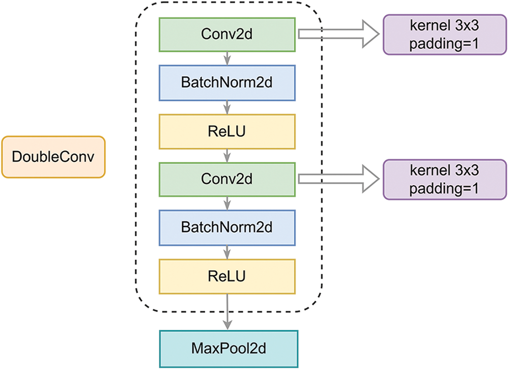
Figure 2: SC-Net structure

The downsampling part can be divided into two groups of sampling modules. The downsampling process is shown clearly in Fig. 3. The first module is original sampling modules. To start with, two 3×3 convolution is used to extract the target features, and after each convolution, batch normalization is used to improve the convergence speed of the model. Then it is activated by ReLu function. Finally, the resolution is reduced by 2×2 maximum pooling with a step length of 2, and the original module is invariable in the third and fourth downsampling. The second sampling modules splices the images before and after double convolution in the column dimension, and then restores the original number of channels through 1×1 convolution. Finally, 2×2 maximum pooling is carried out on the whole Mosaic, and the pooled image is used as the input of the next sampling module. The new module replaces the original first and second sampling modules.

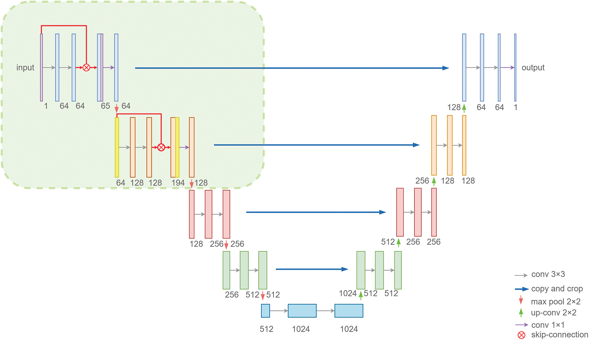
Figure 3: Downsampling

3.2 Combined Loss Function

The hippocampus’s mask makes up a small portion of the background because it is so small in comparison to the rest of the brain. As a result, there is an imbalance between target and background. With the imbalance taken into consideration, we utilized Dice Loss [18] to address the issue of excessively low foreground ratio. The Dice coefficient is a set similarity measurement function that can be used as an index for evaluating results of segmentation. It is a standard representation of the label’s similarity to the segmentation result. The value is between 0 and 1, and the closer it is to 1, the better the segmentation effect is. The procedure for calculating performance is as follows:

Dice=2(Vfcn∩Vmanu)(Vfcn∪Vmanu)(1)

Among them, Vfcn represents the segmentation result of the model, and Vmanu represents the corresponding label. When the Dice Loss is smaller, it means that the similarity between the two pictures is greater, and when the Dice Loss is larger, it means that the sample similarity is smaller. The calculation method of Dice Loss is:

DiceLoss=1−Dice(2)

An important part of our job is to emphasize edge contours more. We use Focal Loss [19] to increase the focus on points that are difficult to segment in order to better concentrate on the segmentation of difficult-to-confirm edges. The procedure for calculating is as follows:

FL(pt)=−α(1−pt)λlog⁡(pt)(3)

pt={pif y = 11−potherwise(4)

Among them, p represents the predicted probability the model provided. pt is used to indicate the closeness between the actual value and the predicted value, and the closer pt is to 1, the more accurate the classification is α represents the category weight, which is used to weigh the imbalance between positive and negative samples. λ represents the weight of difficult samples, which is used to measure difficult samples and easy samples, and increase the attention of difficult samples by adjusting the weight.

We proposed a combined loss function for error calculation by combining the two loss functions previously mentioned and processing the output image with the Canny function [20]. Fig. 4 depicts the process as a whole. Firstly, we directly calculate the Focal Loss between the output mask and the label mask. Secondly, Canny operator is used to perform edge detection on the output image, and obtain the edge map of the output mask. Finally, we calculate the Dice Loss between the edge map and the label mask. The combined loss function can be defined as follows:

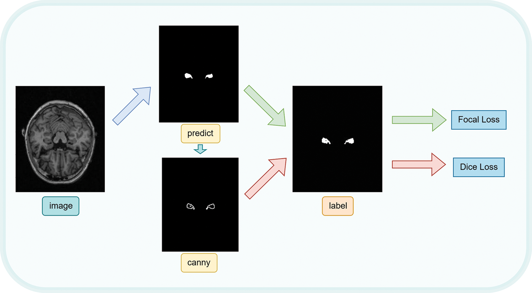
Figure 4: Combination loss function calculation process

Loss=(1−λ)LDice+λLFocal(5)

where λ is a weight that is adjusted based on particular tasks and are used to calculate the impact of marginal loss on total loss. The loss for Dice is represented by LDice, and the loss for Focal is represented by LFocal. Both the background noise caused by the preservation of a entire brain MRI image and the effective improvement in attention to the outline of hippocampus can be achieved through this method.

The specific use process of combined loss is as shown in Fig. 4. The SC-Net model was used to predict the original complete MRI image and obtain the predicted image. Then, canny function is used to detect the edge of the predicted image to obtain the predicted edge contour of the predicted hippocampus. Then, the Focal Loss between the prediction image and the label image and the Dice Loss between the predicted edge profile map and the label image are calculated. Finally, Focal Loss and Dice Loss are combined in a certain proportion to obtain the final mixing loss.

4  Experiment

4.1 Data

Alzheimer’s Disease Neuroimaging Initiative (ADNI, http://adni.loni.usc.edu), which aims to develop clinical, imaging, genetic, and biochemical biomarkers for the early detection and tracking of AD, is provided by MRI data used in this experiment. MRI, PRT, genomics, cognitive function assessment, CSF, and blood biological data have all been collected and organized by ADNI since 2004 in order to uniformly define the major development stages of Alzheimer’s disease. The pace of Alzheimer’s disease prediction, diagnosis, and treatment research is being accelerated by a variety of data, including markers.

4.2 Preprocessing

We converted the obtained data in NIFTI format into an image file by cutting it along the Z axis, obtaining the horizontal plane slice. There are a total of 240 pairs of MRI cross-sectional slices and mask images obtained, 200 of which are used for model training and 40 for testing. MRI cross-sectional images and the masks for the left and right hippocampus that correspond to them are the raw data that are obtained by the following conversion. We merge the left and right masks using image overlay to create the merged label mask image, which allow usto simultaneously segment the left and right hippocampus. We use image flipping to improve the data during the preprocessing phase of this experiment. Before the training, we use Min-max standardization. In this experiment, the original images are not cropped to better capture the influence of other structures’ relative positions on the hippocampus’ position. Instead, the background size of all images are uniformly adjusted so that the entire MRI image can be input and output.

To train the model parameters, 200 pairs of MRI images and their mask counterparts are used as a training set. RMSprop is used as the optimizer to train for 40 epochs. The value of λ in the combined loss function is 0.987, and the best loss function is defined as infinite in the initialization. We use our pre-defined combined loss function as the segmented image’s evaluation index during the training process, and the optimizer is used to update the parameters after each training. The model produces a value between [0, 1] as its final output for each pixel. In order to convert the output image into a binary mask image and classify the pixels as either 0 or 1, we employ 0.5 as the threshold.

4.3 Comparison

After the training is complete, we use the saved best model to verify the test set. Fig. 5 shows the input raw MRI images, labeled mask images, segmented images, and overlays of ground truth and predicted labels during training. It can be seen from the figure that the proposed method’s segmentation contour is more similar to the label contour, allowing it to effectively locate hippocampal structure in the brain MRI image during segmentation.

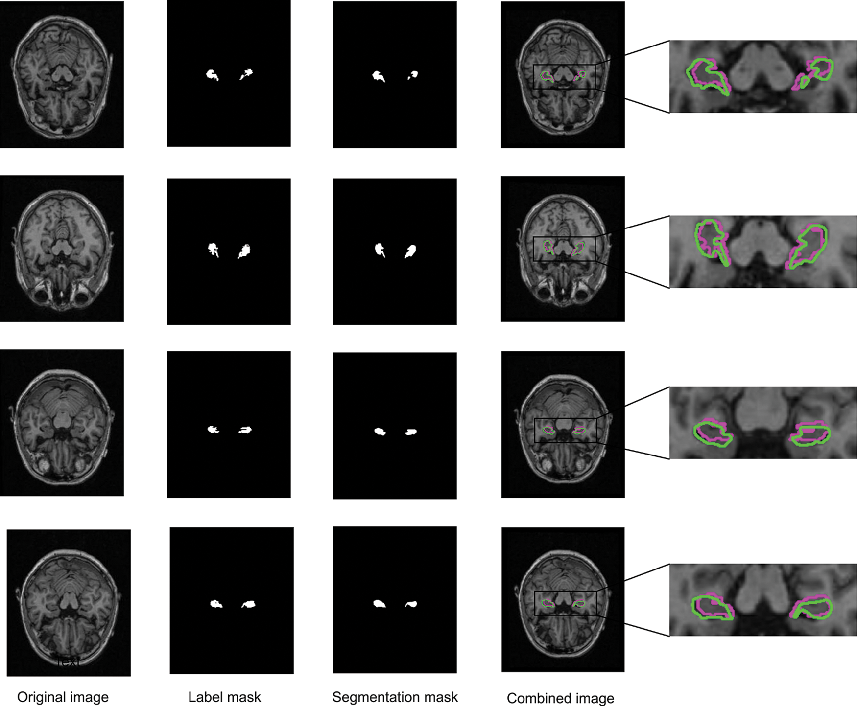
Figure 5: Segmenting results using SC-Net (red is real contour, green is segmented contour)

In the test set, we use Dice, SSIM, Precision, Specificity and Sensitivity as evaluation indicators of the model. SSIM (Structural Similarity) [21] is a measure of the similarity of two images that mimics human perception by focusing primarily on edge and texture similarities. Given two images x and y with the same size, the structural similarity of the two images can be computed as follows:

SSIM(x,y)=(2uxuy+c1)(2σxy+c2)(ux2+uy2+c1)(σx2+σy2+c2)(6)

where ux, uy are the averages, ux2, uy2, σxy are the variances, c1=(k1L)2, c2=(k2L)2, c1 and c2 are constants used to maintain stability. L is the dynamic range of pixel values, k1=0.01, k2=0.03. The range of structural similarity is [−1, 1], and the value of SSIM is 1 when two images are exactly the same.

Precision is used to calculate the proportion of real positive examples in predicted positive examples. The calculation formula is:

Precision=TP(TP+FP)(7)

Specificity is used to represent the predictive ability of negative examples, the expression is:

Specificity=TN(TN+FP)(8)

Sensitivity represents sensitivity, which is used to reflect the predictive ability of positive examples. The calculation formula is:

Sensitivity=TP(TP+FN)(9)

Among them, TP (True Positive) indicates that positive samples are regarded as positive samples, TN (True Negative) indicates that negative samples are regarded as negative samples, FP (False Positive) indicates that negative samples are regarded as positive samples, and FN (False Negative) indicates that positive samples are regarded as negative samples. The samples are deemed to be negative. Table 1 displays our method’s final performance on the test set.

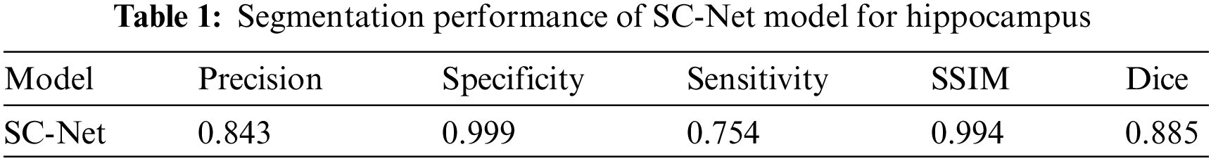
Fig. 6 depicts the change of combined loss function during training. We increased Focal Loss’ weight during adjusting parameter λ. From Fig. 6, we can see that Focal Loss has the greatest impact on the change trend of the loss function, while Dice Loss only has subtle change.

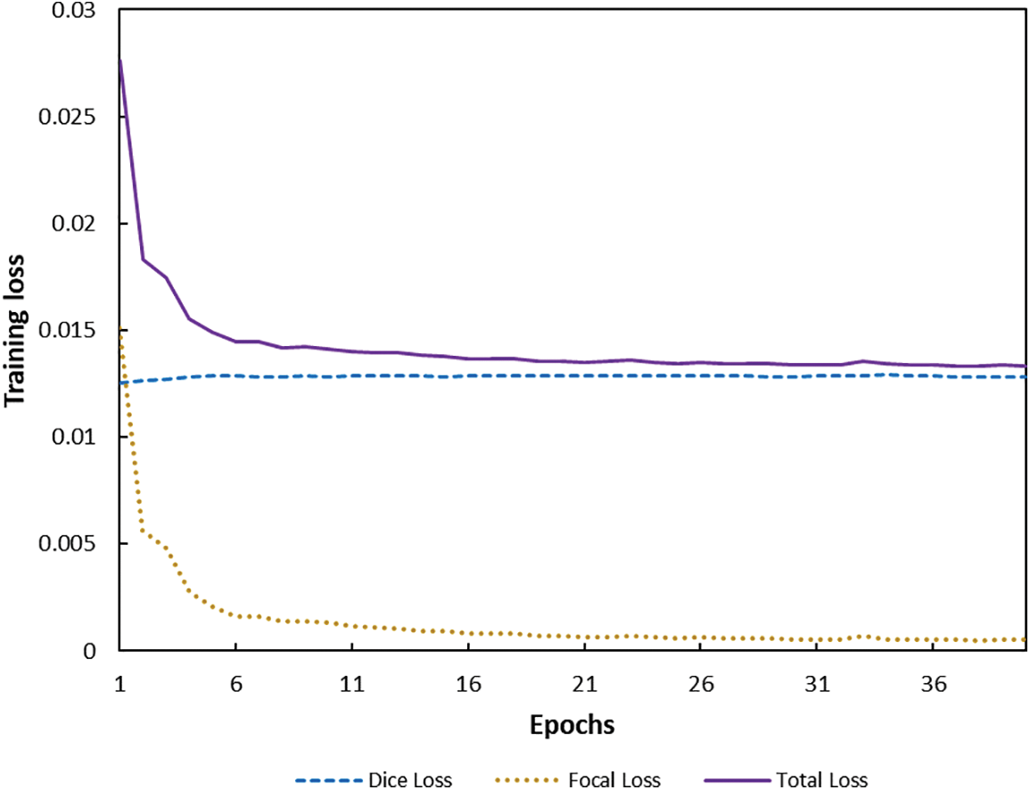
Figure 6: Training loss function

Ablation experiments are implemented to compare U-Net, U-Net+A, U-Net+B, and our proposed model in the same environment. Precision, Specificity, Sensitivity, SSIM, and Dice are used as evaluation indicators to further verify the effectiveness of our proposed model. Table 2 shows the comparison results. It can be seen that our proposed SC-Net outperforms the above models from ablation experiments. The Dice index has increased by 2.7% and the Sensitivity index has increased by 9.2%, respectively. While Precision decreases, Sensitivity and Dice increased after skip connections are added to the first and second downsampling modules, respectively. The decrease of Precision is the result of redundant features being retained. In addition, little target foreground and mis-segmented redundant background lead to increase FP. We define a combined loss function that reduces the impact of background mis-segmentation by detecting edge contours and increases attention to difficult-to-segment regions. From Fig. 7, we can see that the effect of combined loss function reduces the background mis-segmentation problem caused by skip connections retaining redundant features.

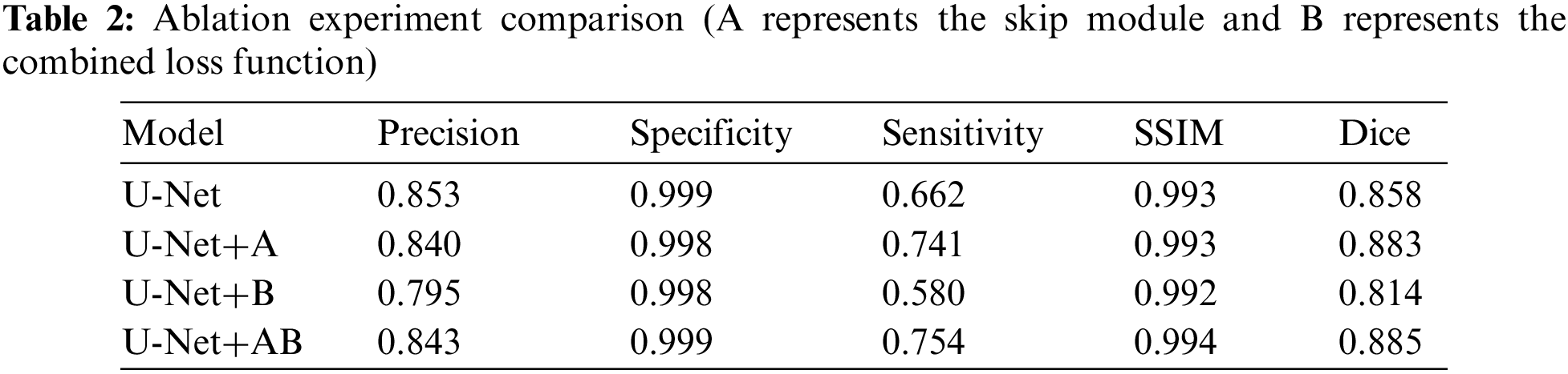
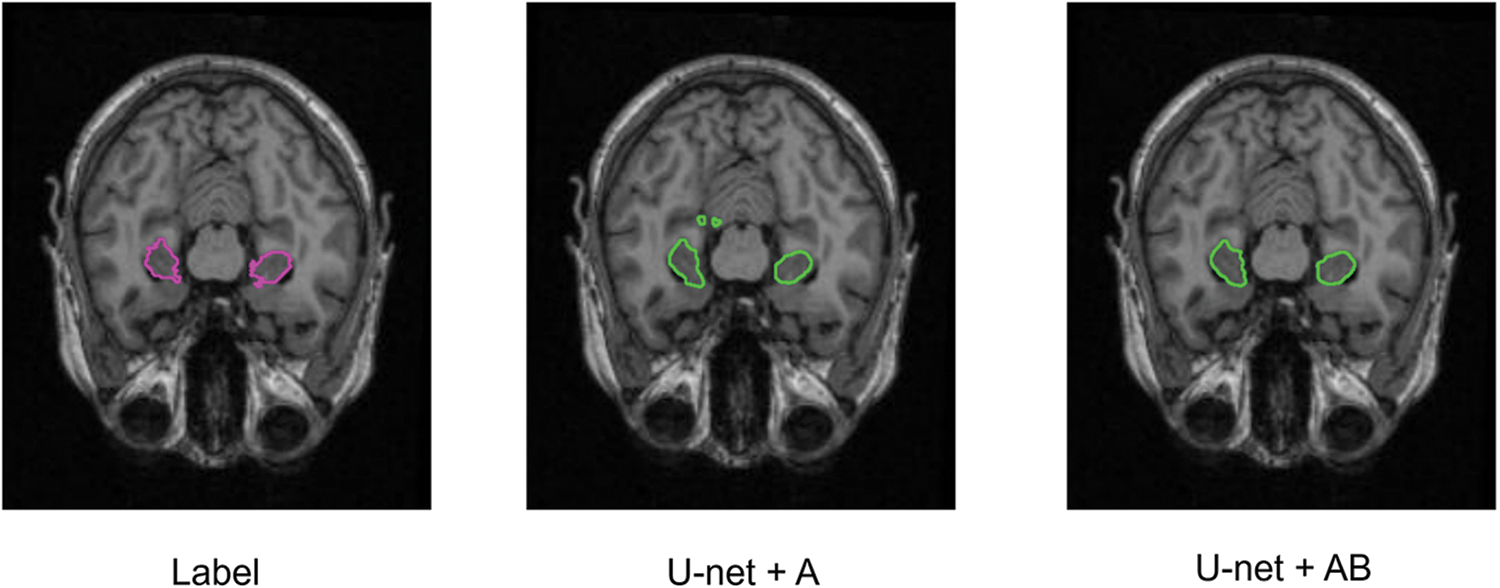
Figure 7: Segmentation of ablation experiment

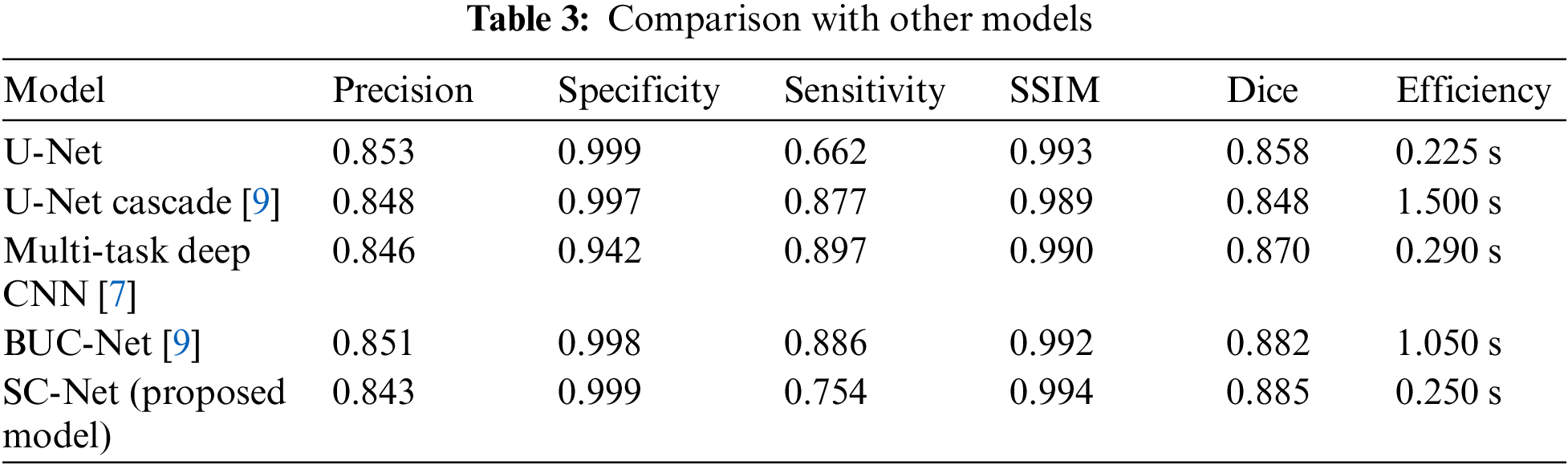
Additionally, we also compared the segmentation performance between SC-Net and other hippocampal segmentation methods. Our proposed SC-Net can directly operate on original MRI images and achieve a higher evaluation indicators, especially perform very well at Dice value and SSIM value. In addition, our model has higher segmentation efficiency due to its lightweight construction, reducing the segmentation time and increasing its segmentation performance greatly. The evaluation index comparison is shown in Table 3.

5  Conclusions and Future Work

In this paper, a new SC-Net model for hippocampus segmentation is proposed to segment and improve the accuracy of hippocampal structure segmentation in human brain magnetic resonance images. First, image features that might have been lost during the first two double convolution phases of the downsampling are preserved by introducing skip connections. In order to further improve the model, the edge loss function is also incorporated into the combined loss function during training. Without local cropping of the hippocampal structure, this method can directly segment MRI images of the brain, and simplify the preprocessing steps. Based on ADNI dataset, extensive experimental results show that our proposed network has performed better. In the future, to better accurately assess the patient’s disease stage, we will consider combining the segmentation model with the classification model and classifying the segmented hippocampus according to shape. Besides, we will consider introducing skip connections and edge constraint methods into different modules according to different segmentation tasks to extend this method.

Acknowledgement: Data used in preparation of this article were obtained from the Alzheimer’s Disease Neuroimaging Initiative (ADNI) database (adni.loni.usc.edu). As such, the investigators within the ADNI contributed to the design and implementation of ADNI and/or provided data but did not participate in analysis or writing of this report. A complete listing of ADNI investigators can be found at: http://adni.loni.usc.edu/wp-content/uploads/how_to_Apply/ADNI_Acknowledgement_List.pdf.

Funding Statement: The authors received no specific funding for this study.

Author Contributions: Xinyi Xiao: Conceptualization, Methodology, Investigation, Formal Analysis, Writing-Original Draft; Dongbo Pan and Jianjun Yuan: Conceptualization, Resources, Supervision, Writing-Review & Editing.

Conflicts of Interest: The authors declare that they have no conflicts of interest to report regarding the present study.

References

1. M. P. Mattson, “Pathways towards and away from Alzheimer’s disease,” Nature, vol. 430, no. 7000, pp. 631–639, 2004. [Google Scholar] [PubMed]

2. Z. Akkus, A. Galimzianova, A. Hoogi, D. L. Rubin and B. J. Erickson, “Deep learning for brain MRI segmentation: State of the art and future directions,” Journal of Digital Imaging, vol. 30, no. 4, pp. 449–459, 2017. [Google Scholar] [PubMed]

3. A. E. Blanken, S. Hurtz, C. Zarow, K. Biado, H. Honarpisheh et al., “Associations between hippocampal morphometry and neuropathologic markers of Alzheimer’s disease using 7 T MRI,” NeuroImage: Clinical, vol. 15, no. Suppl. 3, pp. 56–61, 2017. [Google Scholar] [PubMed]

4. C. Yan, Z. Q. Sun, E. G. Tian, Y. Y. Zhao and X. Y. Fan, “Research progress of medical image segmentation based on deep learning,” Electronic Technology, vol. 34, pp. 7–11, 2021. [Google Scholar]

5. N. Safavian, S. A. H. Batouli and M. A. Oghabian, “An automatic level set method for hippocampus segmentation in MR images,” Computer Methods in Biomechanics and Biomedical Engineering: Imaging & Visualization, vol. 8, no. 4, pp. 400–410, 2020. [Google Scholar]

6. B. Fischl, “FreeSurfer,” NeuroImage, vol. 62, no. 2, pp. 774–781, 2012. [Google Scholar] [PubMed]

7. M. Liu, F. Li, H. Yan, K. Wang, Y. Ma et al., “A multi-model deep convolutional neural network for automatic hippocampus segmentation and classification in Alzheimer’s disease,” NeuroImage, vol. 208,no. 5, pp. 116459, 2020. [Google Scholar] [PubMed]

8. F. Milletari, N. Navab and S. A. Ahmadi, “V-Net: Fully convolutional neural networks for volumetric medical image segmentation,” in 2016 Fourth Int. Conf. on 3D vision (3DV), Stanford, CA, USA, IEEE, pp. 565–571, 2016. [Google Scholar]

9. R. Zhang, W. Zhang, L. Jia, Y. Liu, W. Zhang et al., “Research on automatic delineation of hippocampus assisted by multimodal images based on artificial intelligence,” Chinese Journal of Medical Physics, vol. 1, no. 3, pp. 039, 2022. [Google Scholar]

10. K. M. Hosny, A. M. Khalid, H. M. Hamza and S. Mirjalili, “Multilevel segmentation of 2D and volumetric medical images using hybrid coronavirus optimization algorithm,” Computers in Biology and Medicine, vol. 150, no. 106003, pp. 1–41, 2022. [Google Scholar]

11. E. H. Houssein, D. A. Abdelkareem, M. M. Emam, M. A. Hameed and M. Younan, “An efficient image segmentation method for skin cancer imaging using improved golden jackal optimization algorithm,” Computers in Biology and Medicine, vol. 149, no. 106075, pp. 1–17, 2022. [Google Scholar]

12. J. Long, E. Shelhamer and T. Darrell, “Fully convolutional networks for semantic segmentation,” in Proc. of the IEEE Conf. on Computer Vision and Pattern Recognition, Boston, MA, USA, pp. 3431–3440, 2015. [Google Scholar]

13. K. Simonyan and A. Zisserman, “Very deep convolutional networks for large-scale image recognition,” arXiv preprint arXiv:1409.1556, 2014. [Google Scholar]

14. O. Ronneberger, P. Fischer and T. Brox, “U-Net: Convolutional networks for biomedical image segmentation,” in Medical Image Computing and Computer-Assisted Intervention–MICCAI 2015: 18th Int, Conf,, Munich, Germany, pp. 234–241, 2015. [Google Scholar]

15. C. Li, Y. Tan, W. Chen, X. Luo and F. Li, “ANU-Net: Attention-based nested U-Net to exploit full resolution features for medical image segmentation,” Computers & Graphics, vol. 90, no. 6, pp. 11–20, 2020. [Google Scholar]

16. Z. Zhang, C. Wu, S. Coleman and D. Kerr, “DENSE-INception U-Net for medical image segmentation,” Computer Methods and Programs in Biomedicine, vol. 192, no. 105395, pp. 1–15, 2020. [Google Scholar]

17. Z. Q. Zhu, X. Y. He, G. Q. Qi, Y. Y. Li, B. S. Cong et al., “Brain tumor segmentation based on the fusion of deep semantics and edge information in multimodal MRI,” Information Fusion, vol. 91, no. 1, pp. 376–387, 2023. [Google Scholar]

18. X. Li, X. Sun, Y. Meng, J. Liang and F. Wu, “Dice loss for data-imbalanced NLP tasks,” arXiv preprint arXiv:1911.02855, 2019. [Google Scholar]

19. T. Y. Lin, P. Goyal, R. Girshick, K. He and P. Dollar, “Focal loss for dense object detection,” Proceedings of the IEEE International Conference on Computer Vision, vol. 1, no. 1, pp. 2980–2988, 2017. [Google Scholar]

20. J. Canny, “A computational approach to edge detection,” IEEE Transactions on Pattern Analysis and Machine Intelligence, vol. 1, no. 6, pp. 679–698, 1986. [Google Scholar]

21. Z. Wang, A. C. Bovik, H. R. Sheikh and E. P. Simoncelli, “Image quality assessment: From error visibility to structural similarity,” IEEE Transactions on Image Processing, vol. 13, no. 4, pp. 600–612, 2004. [Google Scholar] [PubMed]