Railway Passenger Flow Forecasting by Integrating Passenger Flow Relationship and Spatiotemporal Similarity

1  Introduction

Railway transportation is an essential link of economic and social ties between all parts of the country and plays a vital role in national development. Passenger transportation by rail has the advantages of high capacity, high speed, suitable price, good safety, and not being easily affected by the weather. While the railway transport system in China is developing at a high speed, new problems have emerged. With the scale of the railway network gradually expanding, the railway network is becoming more and more complex making it hard to schedule a suitable timetable for railway trains. An unreasonable train schedule will cause the problem of too few trains to meet the travel needs of passengers or too many trains to fully utilize resources, resulting in a waste of train resources [1]. Hence, there is an urgent need for a strategy that can meet passenger demand while maintaining high utilization of railway resources, which places high demands on accurate railway passenger flow forecasting.

Analyzing the factors that influence passenger flow changes is necessary to forecast railway passenger flow accurately. The formation of passenger flow is mainly based on the travel needs of individuals. Short-term factors influencing passenger flow include special dates such as holidays or summer and winter vacations and peak seasons of passenger flow in tourist cities. Long-term influencing factors include railway network construction and line station design. The impact of these factors is difficult to quantify precisely; predicting railway passenger flow is a complex and nonlinear problem. However, the trend of railway passenger flow shows consistent patterns of change within a specific period, providing the possibility to predict passenger flow trends.

The resurgence of deep learning can be attributed to the advancements in computer hardware and the development of neural network algorithms. In addition to the basic backpropagation (BP) neural network [2], many deep learning algorithms, Recurrent Neural Network (RNN) [3], and its variants [4] are well suited for handling temporal sequences and are widely used in prediction fields [5]. On the other hand, the inertia principle of railway passenger flow suggests that recent local fluctuations in passenger flow significantly impact future passenger flow. Convolutional Neural Networks (CNN) can extract local features within a large range of data [6], which is ideal for identifying regional passenger flow features in railway passenger flow prediction.

In the railway network, dealing with the complex relationships between stations is challenging when only analyzing the passenger flow of a single station in an individual. This approach fails to consider the interconnections between stations. However, the existing railway passenger flow prediction methods rely on a single station’s historical data to forecast the passenger flow using autocorrelation. These methods are inadequate in promptly reacting to local passenger flow changes, making accurate predictions of future passenger flows difficult.

In this study, we proposed a passenger flow prediction model named Flow-Similarity Attention Graph Convolutional Network (F-SAGCN), which considers the spatial correlation between train stations and captures spatiotemporal correlations of railway passengers for more accurate prediction. To sum up, our contributions can be summarized as follows:

(1)   We construct the passenger flow relations graph (RG) with the help of the historical passenger flow data to reflect the real passenger flow mobility between stations. The effect that other stations have on a station’s passenger flow differs significantly depending on whether they are on the same line or a different line. To improve the predictive accuracy of the model, we constructed an RG to represent these influences.

(2)   We construct the spatiotemporal similarity graph (SG) using the spatiotemporal similarity relationship of passenger flow between stations. In the railway system, certain stations show similar spatiotemporal patterns of passenger flow, which represents a key feature of railway passenger flow that is yet to be fully exploited. To address this issue, we propose an algorithm for quantifying the spatiotemporal similarity of passenger flow, which we use to represent this feature as SG.

(3)   We propose the passenger flow prediction model F-SAGCN. The F-SAGCN can extract passenger flow mobility and spatiotemporal similarity from the constructed graphs and combine them with the station’s temporal characteristics for passenger flow prediction.

(4)   The prediction results and the ablation experiment on a railway bureau’s railway passenger flow data verify the proposed model’s improvement and effectiveness.

The structure of this paper is as follows. Section 2 reviews the related works on passenger flow prediction. Section 3 is about the proposed model F-SAGCN and methods to construct RG and SG. Section 4 is the contrast and ablation experiments and the analysis. Section 5 is summarizing the conclusion and future work.

2  Related Works

The railway is the lifeblood of a country’s national economy, and the effective use of railway resources is closely related to the development of the country, and more efficient use of railway resources has been a prominent and focused research problem.

Traditional methods use the time-series pattern feature to predict passenger flow. Williams et al. [7] used the differential integrated moving average autoregressive model of time series (Autoregressive Integrated Moving Average Model (ARIMA) for predicting urban rail traffic sequences. Then more features were considered in the researchers’ study. Tang et al. [8] used the date of passenger flow and weather attributes of cities for regression prediction of short-term fluctuations in rail passenger flow, and Li et al. [9] conducted a quantitative analysis of factors affecting high-speed rail passenger flow and arranged and combined various features into a support vector machine (SVM). Limited by the technical conditions, these methods are hard to comprehensively analyze the input features or model the relationship between features.

With the development of technology, deep learning has come into the sight of researchers [10–12]. Hosseini et al. [13] build CNN networks to predict passenger flow. According to the characteristics of different deep learning modes Qin et al. [14] integrated an SVM neural network to achieve accurate prediction of traffic flow based on historical traffic data and BP neural network. Ma et al. [15] consider multiple factors as contexts and combined CNN and Long Short-Term Memory (LSTM) for prediction. Many studies have incorporated spatial features to improve prediction accuracy [16–22]. In recent years, many studies [23–25] have proposed deep learning methods based on graph structures. Yu et al. [26] used CNN to capture spatial features and input the vectors after feature extraction into LSTM to extract time features to complete the traffic network flow prediction. Li et al. [27] proposed the diffusion convolutional cyclic neural network, which uses the random walk to model space dependence and a gated cyclic neural network to model time dependence to predict traffic flow. Yu et al. [28] used causal convolution to extract local features in the time dimension and used the emerging graph convolution neural network to aggregate local features in space to predict traffic flow dynamically.

Most existing railway passenger flow prediction studies are based on single-station passenger flow time-series data, which rely strongly on historical passenger flow data. The prediction effect decreases significantly when the data is missing or changes greatly in the short term. Some studies extract temporal and spatial features to improve the prediction effect but ignore the spatial flow of railway passenger flow. When the sending passenger flow of a station increases abnormally, these passengers will be sent to several associated stations. These abnormally increased passenger flows will be expressed in the form of return passenger flow in the future. Many stations have similar patterns in passenger flow fluctuations, while most studies directly use neural network models for feature extraction, without considering the a priori features of similar stations with similar passenger flow fluctuations. Therefore, to improve the accuracy of railway passenger flow prediction, it is essential to consider the spatial flow of passenger flow, as well as the underlying patterns and features of similar stations. This can help in better predicting passenger flows even when data is missing or there are abrupt changes in passenger flow patterns.

3  Method

This paper uses passenger flow mobility and spatiotemporal similarity of inter-station passenger flow to assist in forecasting. We first construct the passenger flow graph based on the inter-station passenger flow movement and prune it using the passenger flow rate. By the passenger flow fluctuation similarity algorithm which aggregated the DTW algorithm and the shape distance algorithm, we construct the spatiotemporal similarity graph. Then, the spatiotemporal features are extracted from the constructed graphs. Finally, we design the F-SAGCN model which introduces the graph attention mechanism and graph convolution layers to fuse the learned features for prediction. The framework of the model is shown in Fig. 1.

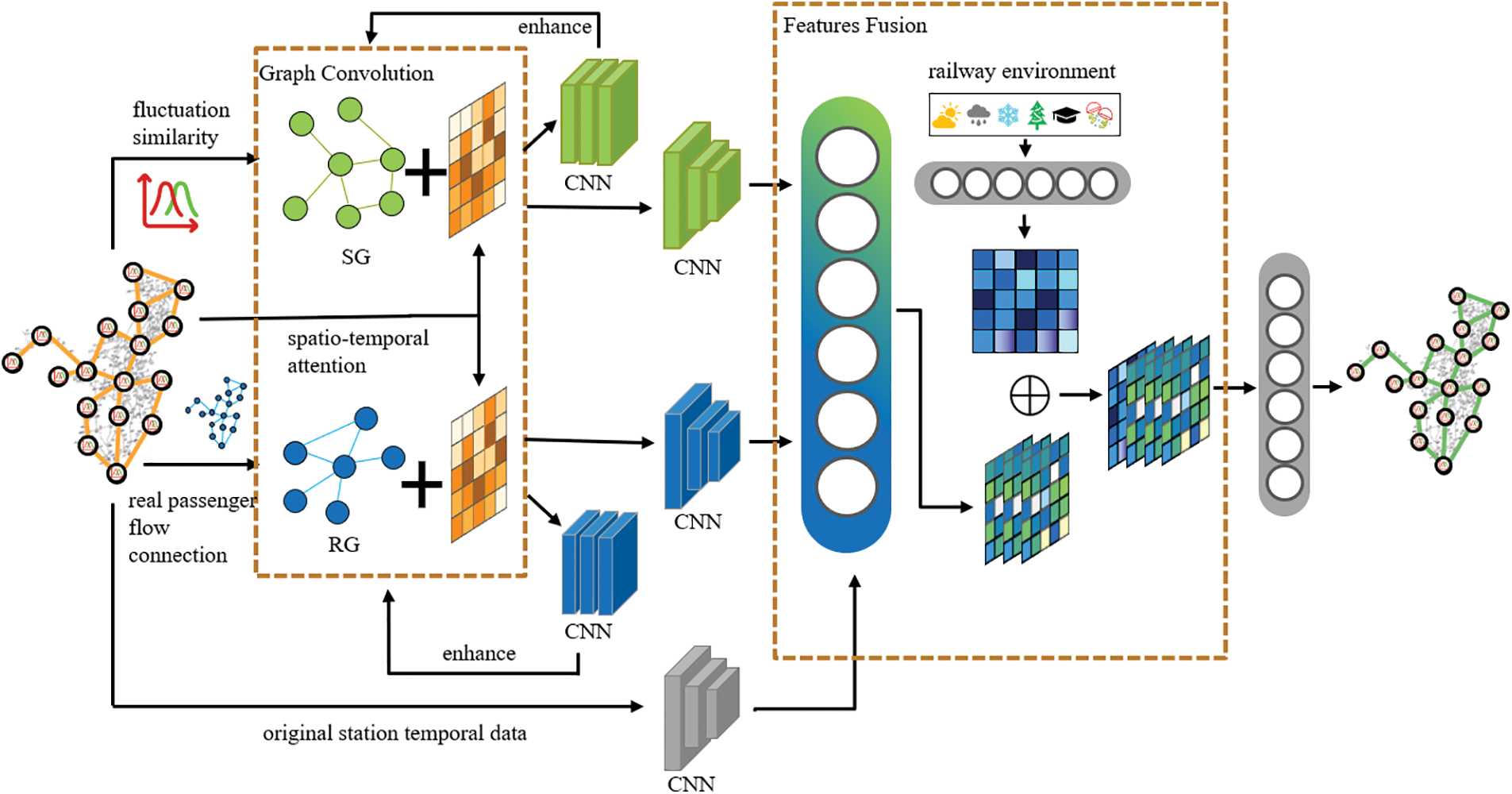
Figure 1: The framework of the F-SAGCN

3.1 Passenger Flow Graph Construction

To model the interaction between individual stations, the first step is to extract the connection of passenger flows between stations in the railway network. For example, the daily passenger flow between station A and station B is large, and when there is an abnormal increase in outgoing passenger flow at station A, and the flow of this abnormal increase is towards station B, then these outgoing passenger flows will be manifested in the form of return passenger flows at stations A and B in the next few days. Therefore, for the prediction model to capture this intuitive, existing passenger flow connection, this paper proposes to construct a passenger flow diagram of the railway.

The passenger flow graph (RG) is established based on the passenger flow relationship in the real railway system, if there is a direct passenger flow from station Ni to station Nj, an edge is established between the vertices of stations Ni and Nj. Finally, the set of RG’s edges is obtained, which is represented by the adjacency matrix and each element of the matrix indicates the edge information. Meanwhile, the OD matrix of passenger flow between stations is calculated. The OD matrix is a matrix containing all stations and the actual passenger flow between any two stations.

With the help of the matrix, RG is pruned by the passenger flow rate to reduce the computation for graph convolution, and avoid too many parameters leading to overfitting while improving the training speed. The calculation of passenger flow rate F is defined as shown in Eq. (1), where flowi→j denotes the passenger flow from the station i to station j, and k is the set of stations with a direct passenger flow relationship at station i.

Fi→j=flowi→j∑kflowi→k,and k∈neibor(i)(1)

The above process is all based on directed graphs. The reason is that when pruning, a passenger flow that has little impact on the larger station may still be able to have an impact on the smaller station on the other side. Therefore, the use of directed graphs still preserves the edge of the smaller station pointing to the larger station and removes the relationship between the two stations completely only when the incoming and outgoing traffic is not important to either station. We will transform the pruned-directed graph to the undirected one when doing the frequency domain graph convolution.

3.2 Spatiotemporal Similarity Graph Construction

The spatiotemporal similarity graph (SG) is established based on the similarity of passenger flow fluctuations with time series between different stations, and this similarity can be precisely measured by the formula. In this paper, we propose PFFS to measure the similarity of passenger flow fluctuations by combining Dynamic Time Warping (DTW) and improved piecewise linear representation (PLR). The stations with similar traffic fluctuations are linked by the passenger flow fluctuation similarity measure algorithm.

The Euclidean distance is widely used to measure the distance between two series, but it has two shortcomings: it cannot determine the similarity of shape and fails to describe the similarity of the magnitude of the trend change. DTW algorithm can align the similar corresponding points of two-time series data by scaling the time series data, and the calculated DTW distance can better measure the similarity of time series shape than Euclidean distance as shown in Fig. 2.

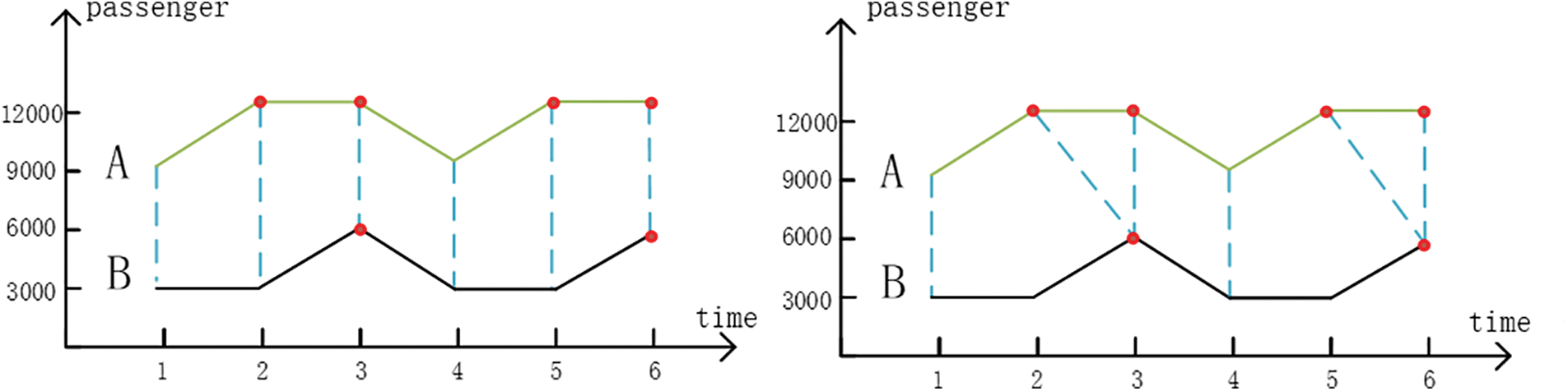
Figure 2: Euclidean distance (left) and DTW (right)

DTW is based on dynamic programming. It calculates the distance matrix D between each point of two sequences and finds the path with the minimum element sum from the upper left corner of the matrix to the lower right corner of the matrix. The m is the length of the passenger flow sequence, and The DTW distance is D(m,m) that can be calculated by Eqs. (2) and (3) as follow.

dis(i,j)=Xi−Yj(2)

D(i,j)=min{D(i−1,j−1),D(i−1,j),D(i,j−1)}+dis(i,j)(3)

DTW is very effective in extracting the similarity of stations with a close base number of passenger flow and approximate changes, but some stations with similar changes (shapes) of passenger flow fluctuation but large differences in values will be difficult to be selected as a result, the improved PLR algorithm is a supplement to the DTW to measure the similarity of passenger flow.

According to the fluctuation, seven patterns of passenger flow change are defined as shown in Table 1.

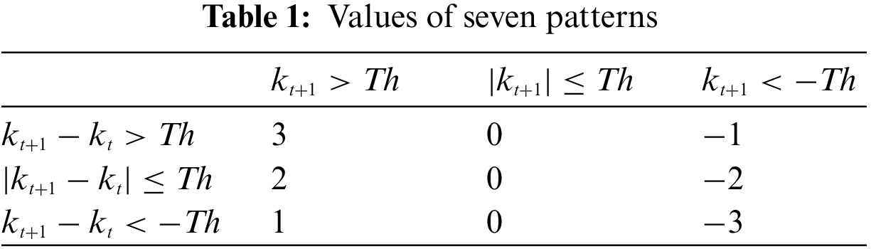
where kt is the slope of the passenger flow sequence at a given time, and Th is the set slope threshold, the fluctuation of randomness in railroad passenger flow generally affects no more than 10% of the daily passenger flow, 0.1 is chosen as our Th threshold. The passenger flow has not changed significantly when the fluctuation does not exceed this threshold. The distance between two pattern sequences (X and Y) is calculated by Eq. (4).

PLR_dis=∑i=1m|Xi−Yi|(4)

After obtaining the similarities calculated by both algorithms, the top five stations closest to the station are picked respectively to establish edge relation. Then, the graphs generated by the two methods are merged to construct the spatiotemporal similarity graph.

3.3 Passenger Flow Prediction Model Based on RG and SG

Based on the passenger flow graph and spatiotemporal similarity graph obtained in the previous section, this paper proposes the spatiotemporal flow prediction model F-SAGCN for predicting the future passenger flow at each station. The model obtains the weight matrix through the spatiotemporal attention, uses graph convolution to extract passenger flow features and spatiotemporal features from the RG and SG, and repeats this process to obtain enhanced passenger flow features and spatiotemporal similarity feature representation through CNN extraction of temporal features. Those features are fused with the temporal features obtained from the convolution of the original station data and the external features obtained from the weather and holidays and fed into the fully connected neural network (MLP) to complete the prediction.

3.3.1 Spatiotemporal Attention

Spatiotemporal attention can assign weights to the passenger flow data to ensure that the feature extraction is focused on the more relevant time points and stations. After calculating the temporal attention, the spatial attention is calculated on it to obtain the spatiotemporal attention. The time attention Tout is calculated as shown in Eq. (5).

Tout =reshape(reshape(X)⋅Softmax(W4⋅σ((XT⋅W1⋅W2)⋅(W3⋅X)+bt)))(5)

where X∈RB×V×F×T is the input, B is the batch size, V is the number of stations, F is the number of features contained in each time step of the station, and T is the temporal length of the input, Wi(i∈N) is parameter matrix. In the same way, spatiotemporal attention can be obtained by taking the temporal attention output Tout as input and calculating the correlation in the spatial dimension. The Laplace matrix L is calculated according to Eq. (6).

L=D−A{Dii=∑jAij,andj∈V}(6)

where D is the degree matrix of the graph and A is the adjacency matrix of the graph. The adjacency matrix A of the RG and the SG has been obtained in the data preprocessing.

3.3.2 Graph Convolution

We use frequency domain graph convolution at each time point to extract features of the station neighbors. Analogous to the traditional convolution to deduce Eq. (7), we can calculate the eigenvalues and eigenvectors for the Laplace matrix L, L=UΛUT, U is the eigenvector matrix, Λ is the eigenvalue matrix.

(g∗x)=U(UTg⊙UTx)=UgθUTx(7)

where UTg is the convolution kernel in the graph convolution operation, denoted as gθ, and x∈RB×V×T is the data of each time slice extracted for the input X, representing the graph signal at each time point. To reduce the computational effort, inspired by the previous work [29], we simplify the computation of the convolution kernel using Chebyshev polynomials, and the final formula introduced to compute the convolution kernel is shown in Eq. (8).

gθ≈∑k=0K−1θkTk(Λ~),andΛ~=2Lλmax−IN(8)

where θk is a polynomial coefficient, Tk(Λ~)=2Λ~Tk−1(Λ~)−Tk−2(Λ~), and T0(Λ~)=1, T1(Λ~)=Λ~, λmax is the maximum value in the eigenvalues, IN is the diagonal matrix with the same shape as Λ~ and K is the highest order of the Chebyshev polynomial. Aggregate features of neighboring nodes in the past moments are captured by graph convolution kernel aggregation features.

3.3.3 Passenger Flow Features Fusion

To get the complete real passenger flow characteristics, it is necessary to fuse the previously gained passenger flow characteristics, spatiotemporal similarity characteristics as well as passenger flow timing characteristics, and rail environment characteristics. To effectively capture the passenger flow temporal features, CNN is used to perform temporal feature extraction on the feature vectors after graph convolution, and the process of graph convolution and temporal feature extraction is repeated to strengthen the features as in Eqs. (9) and (10). In addition, the original passenger flow data are subjected to temporal feature extraction to ensure the integrity of the temporal features.

ST_capture(X,G)=ReLU(Φ∗ReLU(g(G)∗attention(X)))(9)

Xout=ST_capture(ST_capture(…ST_capture(X,Gr),Gr),Gr)(10)

The external environmental features of railroads, such as weather, holidays, festivals, etc., are discretized by One-hot coding and mapped into external feature vectors E. We stack the vector E through fully connected neural networks. Finally, the passenger flow feature fusion is carried out. We first fuse the feature vectors obtained from the two graphs with the original temporal features into a two-layer fully connected neural network as the initial feature vectors. Then we splice the fused feature with the external feature vector into the fully connected neural network. At last, all features are fused to obtain the final prediction results as in Eq. (11).

Predict=MLP(MLP(ReLU(Φ∗Xr),ReLU(Φ∗Xs),ReLU(Φ∗X))⊕E)(11)

The loss function in time series prediction generally chooses the mean of square error (L2 loss) or absolute average error (L1 loss), the former is influenced by the large value of the error, and the latter is easy to affect the final convergence process of the neural network because the gradient is not smooth. In this paper, we choose smoothL1, which is in the middle of the two, as the loss function, which can combine some advantages of L1 loss and L2 loss, and its formula is as follows Eq. (12).

smoothL1={0.5x2,|x|≤1|x|−0.5,|x|>1(12)

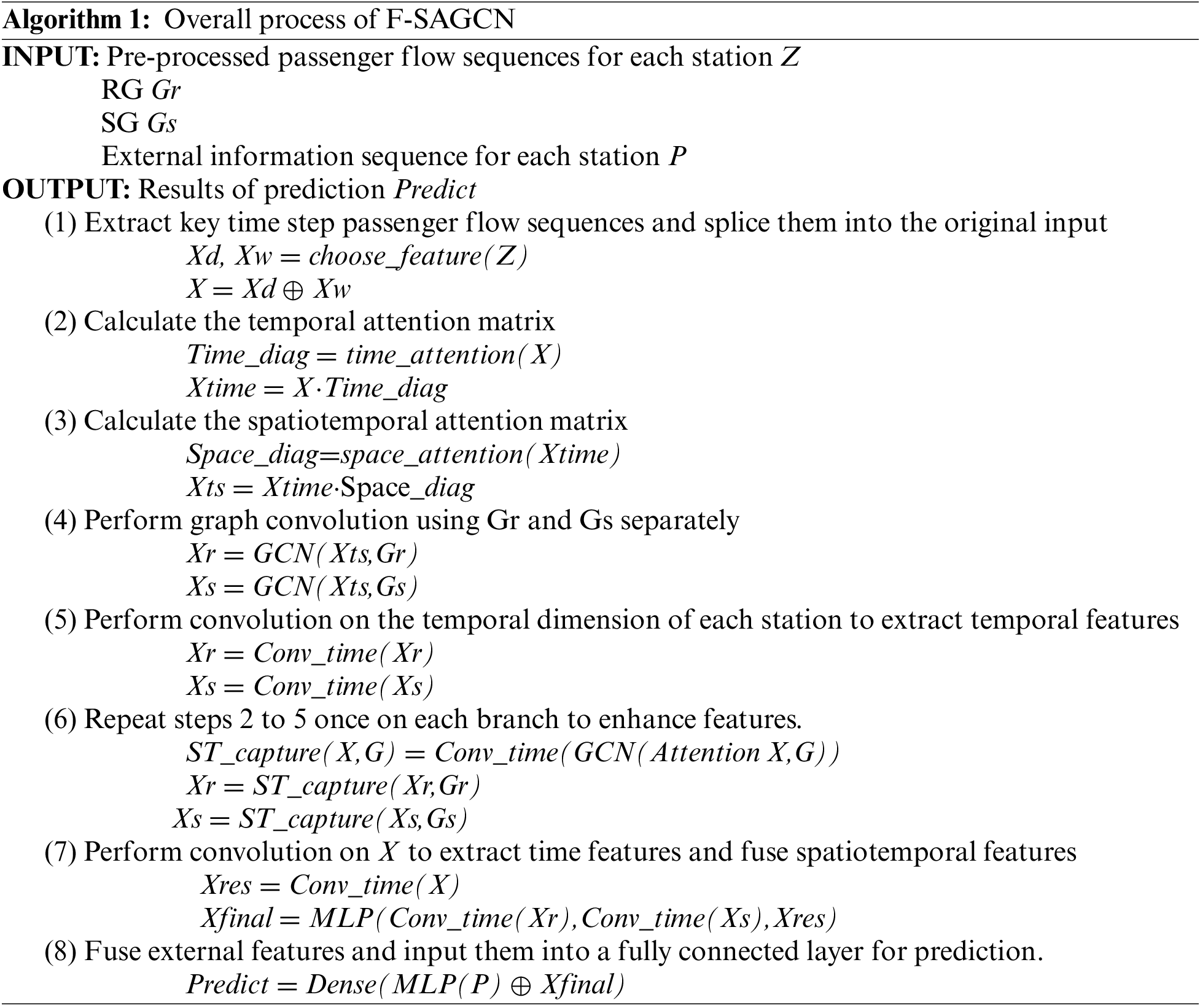
The overall process of our proposed F-SAGCN framework is outlined in Algorithm 1.

4  Experiments

The experimental machine in this paper has the CPU model AMD Ryzen 7 5800H and GPU model RTX3060 and uses pytorch+CUDA-11.2 as the deep learning framework. The learning rate in the experiments is set to 0.001, the loss function is smoothL1, and 350 epochs are iterated.

4.1 Data Quality Improvement

The raw passenger flow data needs to be quality cleaned and corrected to extract high-quality passenger flow characteristics. Some stations have very small daily passenger flows, but the fluctuation is very sharp, the randomness is too large, and the impact on ticket allocation is small. These small stations with small impacts but great numbers can increase the complexity of the model, reduce the model performance, and provide limited help to improve the model’s accuracy. Missing or abnormal values in the passenger flow data will greatly affect the training effect of the neural network which is unavoidable during the statistical process. The difference between the values of passenger flow at each station is large, and the direct input of the original values will affect the training speed and accuracy of the model.

For the missing values, using the cyclical fluctuation characteristics of passenger flow, we calculate the average change value of the week type in the recent three cycles. Because the railway passenger flow is most affected by the recent historical passenger flow, we can get the approximate estimate of the missing values by adding the average change value with the previous day’s passenger flow as Eq. (13).

Xt=Xt−1+13∑i=13(Xt−7i−Xt−7i−1)(13)

For abnormal values, which originate from system failure resulting in record loss but are different from missing values, there are still records of passenger tickets for that day, and generally show an abnormal decrease in passenger flow, which is obviously beyond the normal range of variation. In this paper, we adopt the 3σ detection method to detect outliers and use the method of calculating missing values to replace them. For the passenger flow data with a large gap, the data are standardized to adjust the data of each dimension and each station to the same magnitude to speed up the convergence of the algorithm to the optimal solution.

4.2 Passenger Flow Forecast

In this paper, the following three general prediction metrics are used to measure the model effect, mean absolute error (MAE), root mean square error (RMSE), and mean absolute percentage error (MAPE). To visualize the prediction effect of the method in this paper, the prediction results of some stations and the actual passenger flow are represented visually in Fig. 3.

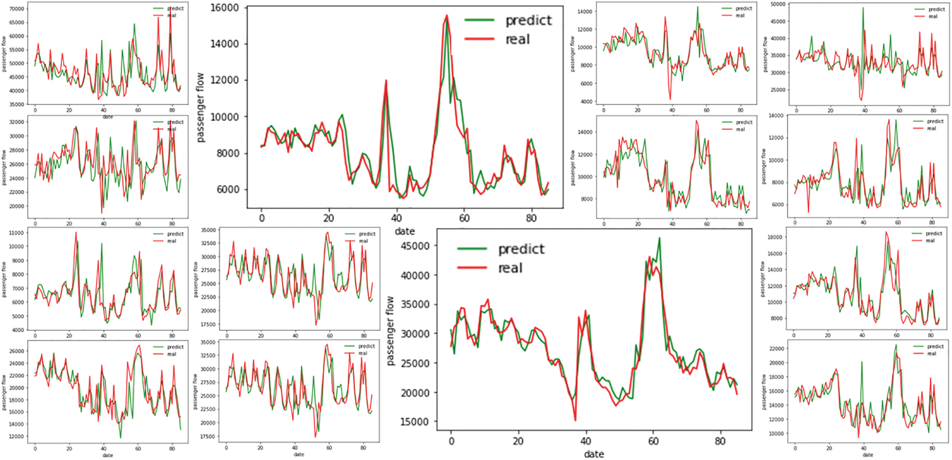
Figure 3: Some stations’ forecast results

4.3 Comparative Experiments

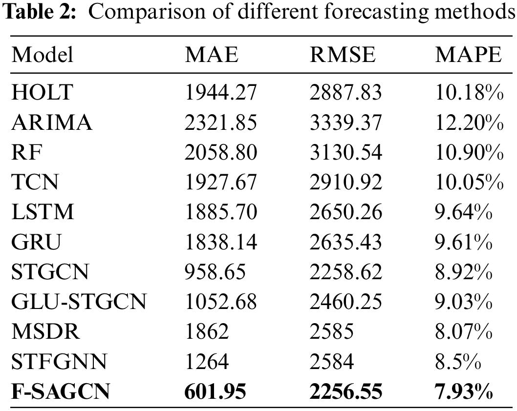
To verify the improvement effect of F-SAGCN in railway passenger flow prediction accuracy, several existing railway passenger flow prediction methods were used to conduct experiments on the railway passenger flow dataset extracted in this paper. The results are shown in Table 2. Since the model predicts 46 stations simultaneously, the values of the three metrics in Table 2 are the average of all stations.

(1) HOLT-WINTER [30]: Giving different weights to data in different periods, it is suitable for non-stationary time series with periodic changes and linear fluctuations and adding a seasonal cycle term to the exponential smoothing method, so that the model can handle the situation of multi-period coexistence.

(2) ARIMA [7]: Difference-integrated moving average autoregressive model, which integrates the autoregressive model, and moving average model, and uses the difference to obtain a smooth time series for forecasting, simple to use and stable effect, is one of the most used time series forecasting models.

(3) RF [31]: Random Forest algorithm, through the input of a variety of features to build different decision trees, integrated many decision trees to form a better effect of the classifier. The advantage is that it can handle higher dimensional inputs with higher accuracy and fast learning speed. In this paper, external features, recent week data, periodic data, etc. are used as features input to the random forest.

(4) TCN [32]: Temporal Convolutional Network, a convolutional neural network that specializes in time series problems, by using convolutional kernels to regularly scan data at earlier time points to extract the desired features, and finally incorporating a residual connection structure.

(5) LSTM [4]: Long Short-Term Memory Network, based on the recurrent neural network RNN with gating structures, solves the problem of the long-term dependence on time-series data that is difficult to retain and is an indispensable structure for many time-series data studies at present.

(6) GRU [33]: GRU is a variant of LSTM, which simplifies the three gating functions in LSTM into update gates and reset gates to retain the ability to deal with long-term dependence while reducing the number of parameters, and the speed is generally better than LSTM due to the simple structure.

(7) STGCN [34]: Spatiotemporal graph convolutional network, consisting of one-dimensional temporal convolution plus graph convolutional neural network, effectively captures comprehensive spatiotemporal correlation by modeling multi-scale traffic networks, and has very good results on many traffic datasets. STGCN has not yet been applied to railway data, and we use the RG as the graph structure to implement the STGCN model for experiments.

(8) GLU-STGCN [28]: A model based on STGCN, designed for traffic flow prediction, with gated linear units added among the causal convolution of temporal sequences, which can also be used for general spatiotemporal sequence learning.

(9) MSDR [35]: Multi-Step Dependency Relation, a new variant of recurrent neural network. Instead of only looking at the hidden state from only one latest time step, MSDR explicitly takes those of multiple historical time steps as the input of each time unit.

(10) STFGNN [36]: Spatial-Temporal Fusion Graph Neural Networks could effectively learn hidden spatial-temporal dependencies by a novel fusion operation of various spatial and temporal graphs, treated for different time periods in parallel. Meanwhile, by integrating this fusion graph module and a novel gated convolution module into a unified layer parallelly, STFGNN could handle long sequences by learning more spatial-temporal dependencies with layers stacked.

Traditional time series methods are generally lower in accuracy than deep learning methods, HOLT model is the best effect of traditional time series methods but compared with the less effective TCN method in deep learning, although slightly better performance in RMSE index, but MAE, MAPE is still a difference of 16.6% and 0.13%, than the method of this paper is a difference of 1342.32% and 2.25%. The traditional time series method only focuses on a single time dimension of a single station, without considering the variable external influences, and can only be fitted with artificially set parameters, which is difficult to cope with the nonlinear fluctuation characteristics, and the fixed parameters also make it difficult for the algorithm to make a timely response to the dynamic data.

LSTM and CNN have commonly used feature capture structures, one is good at capturing long-term time-dependent and the other is good at capturing local variation features. In this experiment, both methods train models for a single station and extract single-station time-series features for prediction. The errors of TCN increased by 1325.72%, 654.37%, and 2.12% in MAE, RMSE, and MAPE, and LSTM increased by 1283.75%, 393.71%, and 1.71% compared with this paper because they did not exploit the passenger flow relationship and passenger flow similarity between stations, and it was difficult to respond to the influence outside their historical data.

STGCN and GLU-STGCN are new results of graph neural network applied to urban traffic flow prediction. The addition of the graph neural network enables the model to use spatial information in spatiotemporal data, and the passenger flow graph is tested as the graph structure in this paper. decreases by 450.73% and 1.1%.

4.4 Ablation Experiments

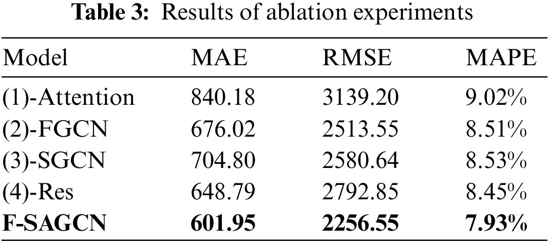
To verify the validity of each part of this model, the ablation experiment is designed in this paper, and the complete model is made to be disassembled as follows.

(1)   Remove the spatiotemporal attention module.

(2)   Remove the branch that extracts the influence of passenger flow (without using the RG).

(3)   Remove the branch of extracting the influence of passenger flow similarity (without using the SG).

(4)   Remove the spatiotemporal influence fusion module (remove the convolution branch of the original data).

After removing these modules separately, the model is used to predict future passenger flows to analyze the impact of the modules on the overall model effect.

As shown in Table 3, removing the spatiotemporal attention module decreases the ability to select the validity of neighboring stations at different time steps, all three error indicators increase, and the RMSE increases by a large amount, reaching 3139.2. Removing the passenger flow diagram prevents the model from targeting and aggregating the features of stations with direct passenger flows, and the MAE and MAPE increase to 676.02% and 8.51%, respectively. By removing the spatiotemporal similarity map and only using the passenger flow map for graph convolution, the model can only obtain information from stations with direct passenger flow. The spatiotemporal similarity map gives the model the ability to learn the common features of stations with similar fluctuations, achieving a migration learning-like effect, and after the model loses this ability, MAE and MAPE increase significantly to 704.8% and 8.53%. Removing the spatiotemporal influence fusion module, the model can only predict by aggregated features of other stations and loses the focus on the most important own temporal features after multiple feature extraction, and the accuracy decreases, and the increase of RMSE and MAPE is more obvious compared to MAE, indicating an increase of extreme values and over-reliance on the features of related stations and deviation from own temporal order.

Meanwhile, the experiments also recorded the changes in the training and validation set losses of the ablation model during the training process, as shown in Fig. 4.

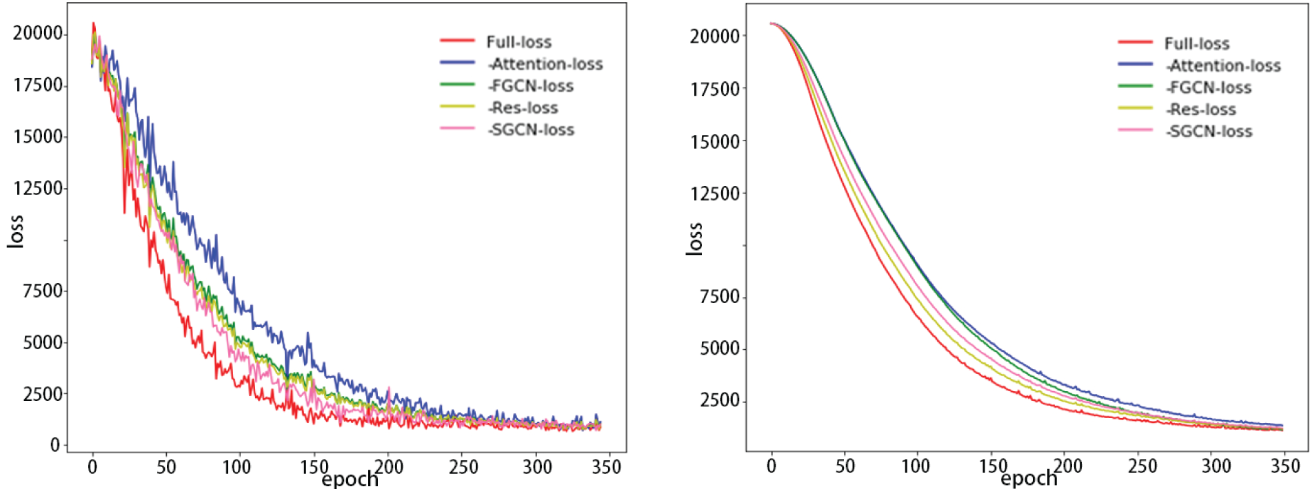
Figure 4: Training set (left) and test set loss (right)

The curves in the figure show that the convergence positions of several ablation models are similar, but the variation of the loss rate shows that the loss of the model that integrates all modules decreases the fastest, and finally the lowest loss can be reached in several ablation methods, and if any of the modules is removed will affect the convergence speed and accuracy of the model, thus verifying the validity of each part of this model.

4.5 Parameter Experiments

To validate the robustness of the model, we do several studies on the model’s parameters and process.

(1) The pruning on RG construct.

To reduce computation, avoid overfitting and improve the training speed, we have pruned the RG. We have researched to analyze the effect of pruning on the speed of the model and accuracy. From Table 4, we can see that the pruning reduces the complexity of the graph convolution.

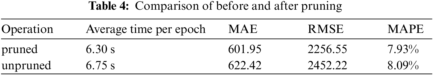
The average elapsed time of each epoch is reduced by 0.45 s. The improvement of the metrics after pruning shows that the edges with weak passenger flow correlation decrease accuracy.

(2) Similarity threshold

To retain sufficient similarity relationships for SG, we do experiments to determine the appropriate threshold. We fixed other parts of the model unchanged and only changed the value of K during RG construction to find the appropriate value of K. The comparison results are shown in Fig. 5.

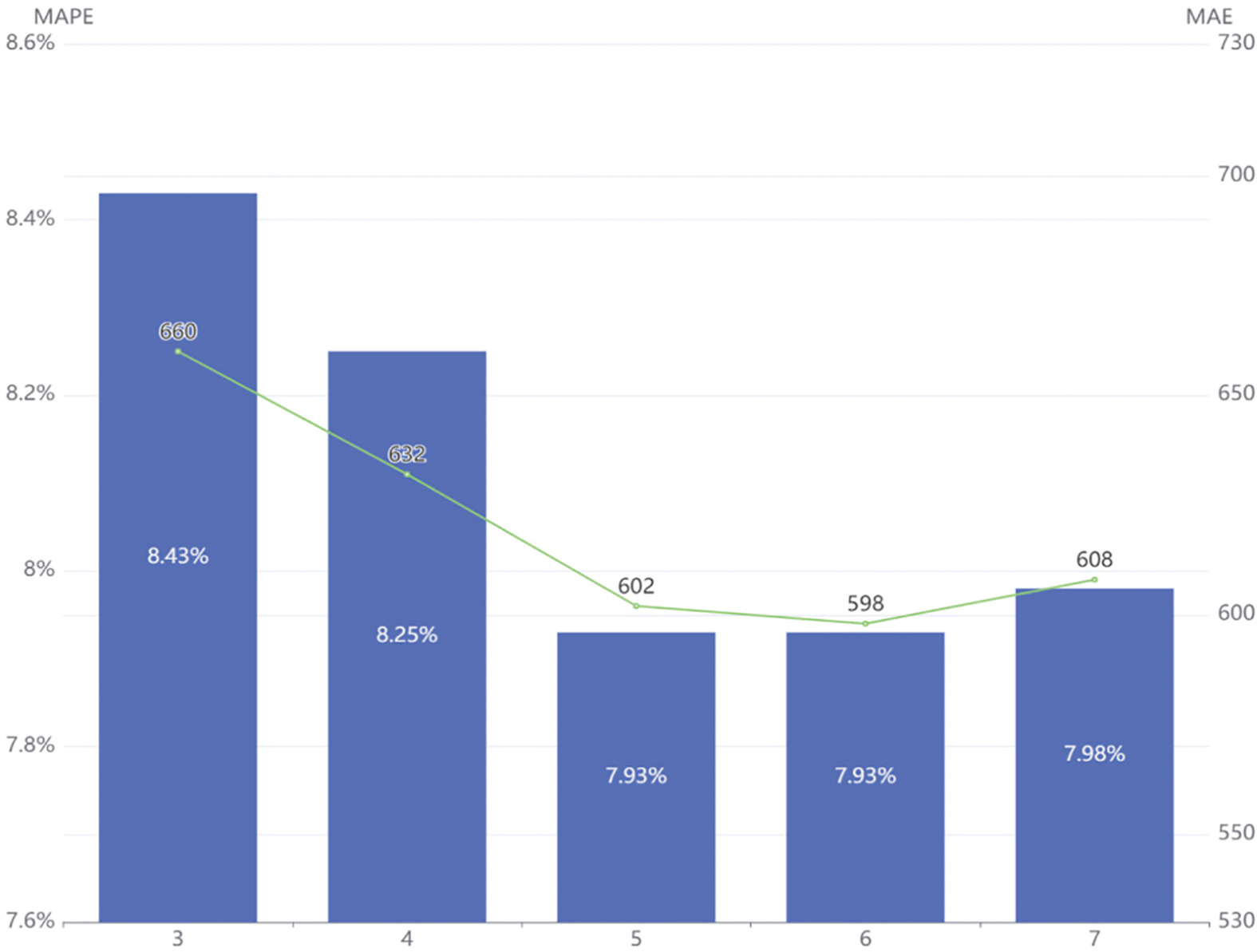
Figure 5: Comparison of threshold selection of similarity relation

As K increased, both MAE and MAPE initially decreased before increasing. This suggests that the additional similarity relationships were valid and helped the model extract more effective features. However, when K reached seven, MAE and MAPE began to increase, indicating that the newly added similarity relationships were no longer improving the model’s predictive ability. The increase in K may have resulted in the selection of stations with lower similarity or a more complex graph structure, leading to overfitting. Based on experimental results, K = 6 resulted in the lowest comprehensive MAE and MAPE, but increasing K led to a more complex SG structure and slower training speed with limited improvement compared to K = 5. Therefore, we selected K = 5 as the threshold for establishing the spatiotemporal similarity graph.

(3) Model parameter

To preprocess the input data, we concatenated adjacent time steps and selected critical time steps from the first two periods. Insufficient input length may result in insufficient historical information, while excessive length can introduce redundant information. In order to determine the optimal length of adjacent time steps, we conducted an experiment, and the results are illustrated in Fig. 6.

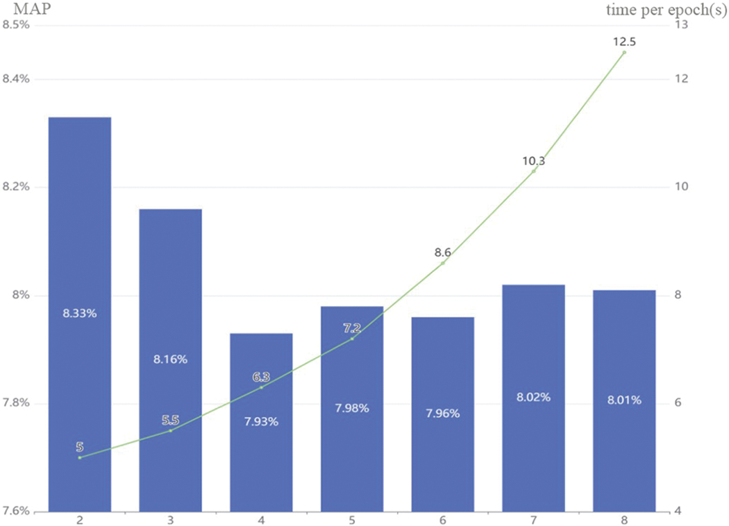
Figure 6: Comparison of different adjacent time steps

The amount of information contained in the input data increases as the length increases and reaches its lowest error point at 4. Thereafter, the mean absolute percentage error (MAPE) remains relatively stable. However, as the time step continues to increase, the size of the data significantly increases and slows down the training speed, especially after 6. To balance training speed and accuracy, we ultimately chose 4 as the length of the input neighborhood time step.

5  Conclusion

In this paper, we propose a novel approach for passenger flow prediction, named F-SAGCN, which employs the spatiotemporal characteristics and the station’s passenger flow characteristics of the railway between each station together for prediction. Specifically, we learn the single-step prediction results from the spatiotemporal sequence data of all stations and extract the historical passenger flow features from neighboring stations as an additional influence on its passenger flow based on the idea of residuals. Then we fuse the fluctuating characteristics of the station’s passenger flow and the spatiotemporal features, obtaining the final passenger flow prediction. The overall prediction effect of the model outperforms previous methods.

The F-SAGCN model achieves promising performance under the existing conditions and will be further improved in the following aspects in future work. On the one hand, we consider using a priori knowledge to introduce the magnitude and direction of passenger flow and spatiotemporal similarity for better matching the actual passenger flow characteristics. On the other hand, we consider dynamically generating the passenger flow map in the configuration via the OD matrix of daily passenger flow between stations which can effectively improve the prediction accuracy and simplifies the computational difficulty of the model.

Funding Statement: The authors received no specific funding for this study.

Conflicts of Interest: The authors declare that they have no conflicts of interest to report regarding the present study.

References

1. K. Wen, G. Zhao, B. He, J. Ma and H. Zhang, “A decomposition-based forecasting method with transfer learning for railway short-term passenger flow in holidays,” Expert Systems with Applications, vol. 189, no. 3, pp. 116102, 2022. [Google Scholar]

2. D. Zhang and L. Wang, “Passenger flow forecast of urban rail transit based on BP neural networks,” in 2011 3rd Int. Workshop on Intelligent Systems and Applications, Wuhan, China, pp. 1–4, 2011. [Google Scholar]

3. L. R. Medsker and L. C. Jain, “Recurrent neural networks,” Design and Applications, vol. 5, pp. 64–67, 2001. [Google Scholar]

4. S. Hochreiter and J. Schmidhuber, “Long short-term memory,” Neural Computation, vol. 9, no. 8, pp. 1735–1780, 1997. [Google Scholar] [PubMed]

5. J. Donahue, L. Anne Hendricks, S. Guadarrama, M. Rohrbach, S. Venugopalan et al., “Long-term recurrent convolutional networks for visual recognition and description,” in IEEE Conf. on Computer Vision and Pattern Recognition, Boston, MA, USA, pp. 2625–2634, 2015. [Google Scholar]

6. M. D. Zeiler and R. Fergus, “Visualizing and understanding convolutional networks,” in Computer Vision—ECCV 2014: 13th European Conference, Zurich, Switzerland, Springer International Publishing, pp. 818–833, 2014. [Google Scholar]

7. B. M. Williams and L. A. Hoel, “Modeling and forecasting vehicular traffic flow as a seasonal ARIMA process: Theoretical basis and empirical results,” Journal of Transportation Engineering, vol. 129, no. 6, pp. 664–672, 2003. [Google Scholar]

8. L. Tang, Y. Zhao, J. Cabrera, J. Ma and K. L. Tsui, “Forecasting short-term passenger flow: An empirical study on Shenzhen metro,” IEEE Transactions on Intelligent Transportation Systems, vol. 20, no. 10, pp. 3613–3622, 2018. [Google Scholar]

9. W. Li, L. Sui, M. Zhou and H. Dong, “Short-term passenger flow forecast for urban rail transit based on multi-source data,” EURASIP Journal on Wireless Communications and Networking, vol. 2021, no. 1, pp. 9, 2021. [Google Scholar]

10. U. Ahmed, G. Srivastava and J. C. -W. Lin, “Reliable customer analysis using federated learning and exploring deep-attention edge intelligence,” Future Generation Computer Systems, vol. 127, no. 3, pp. 70–79, 2022. [Google Scholar]

11. Y. Shao, J. C. -W. Lin, G. Srivastava, A. Jolfaei, D. Guo et al., “Self-attention-based conditional random fields latent variables model for sequence labeling,” Pattern Recognition Letters, vol. 145, no. 6, pp. 157–164, 2021. [Google Scholar]

12. J. C. -W. Lin, Y. Shao, Y. Djenouri and U. Yun, “ASRNN: A recurrent neural network with an attention model for sequence labeling,” Knowledge-Based Systems, vol. 212, no. 1, pp. 106548, 2021. [Google Scholar]

13. M. Khajeh Hosseini and A. Talebpour, “Traffic prediction using time-space diagram: A convolutional neural network approach,” Transportation Research Record, vol. 2673, no. 7, pp. 425–435, 2019. [Google Scholar]

14. H. Qin and W. Zhang, “Short-term traffic flow prediction and signal timing optimization based on deep learning,” Wireless Communications and Mobile Computing, vol. 2022, no. 1, pp. 1–11, 2022. [Google Scholar]

15. D. Ma, X. Song and P. Li, “Daily traffic flow forecasting through a contextual convolutional recurrent neural network modeling inter-and intra-day traffic patterns,” IEEE Transactions on Intelligent Transportation Systems, vol. 22, no. 5, pp. 2627–2636, 2020. [Google Scholar]

16. W. Xu, Y. Qin and H. Huang, “A new method of railway passenger flow forecasting based on spatio-temporal data mining,” in Proc. The 7th Int. IEEE Conf. on Intelligent Transportation Systems (IEEE Cat. No. 04TH8749), Washington, WA, USA, pp. 402–405, 2004. [Google Scholar]

17. H. Yao, F. Wu, J. Ke, X. Tang, Y. Jia et al., “Deep multi-view spatial-temporal network for taxi demand prediction,” Proceedings of the AAAI Conference on Artificial Intelligence, vol. 32, no. 1, pp. 2588–2595, 2018. [Google Scholar]

18. R. Chawuthai, K. Pruekwangkhao and T. Threepak, “Spatial-temporal traffic speed prediction on Thailand roads,” in 2021 7th Int. Conf. on Engineering, Applied Sciences and Technology (ICEAST), Pattaya, Thailand, pp. 58–62, 2021. [Google Scholar]

19. L. Zhang, G. Zhu, P. Shen, J. Song, S. Afaq Shah et al., “Learning spatiotemporal features using 3DCNN and convolutional LSTM for gesture recognition,” in Proc. of the IEEE Int. Conf. on Computer Vision Workshops, Venice, Italy, pp. 3120–3128, 2017. [Google Scholar]

20. X. Xiong, H. Wu, W. Min, J. Xu, Q. Fu et al., “Traffic police gesture recognition based on gesture skeleton extractor and multichannel dilated graph convolution network,” Electronics, vol. 10, no. 5, pp. 551, 2021. [Google Scholar]

21. Y. Li, J. Lang, L. Ji, J. Zhong, Z. Wang et al., “Weather forecasting using ensemble of spatial-temporal attention network and multi-layer perceptron,” Asia-Pacific Journal of Atmospheric Sciences, vol. 57, no. 3, pp. 533–546, 2021. [Google Scholar]

22. S. Wang, Y. Li, J. Zhang, Q. Meng, L. Meng et al., “PM2.5-GNN: A domain knowledge enhanced graph neural network for PM2.5 forecasting,” in Proc. of the 28th Int. Conf. on Advances in Geographic Information Systems, New York, NY, USA, pp. 163–166, 2020. [Google Scholar]

23. J. Wang, X. Kong, W. Zhao, A. Tolba, Z. Al-Makhadmeh et al., “STLoyal: A spatio-temporal loyalty-based model for subway passenger flow prediction,” IEEE Access, vol. 6, pp. 47461–47471, 2018. [Google Scholar]

24. J. Ye, J. Zhao, K. Ye and C. Xu, “How to build a graph-based deep learning architecture in traffic domain: A survey,” IEEE Transactions on Intelligent Transportation Systems, vol. 23, no. 5, pp. 3904–3924, 2020. [Google Scholar]

25. W. Jiang and J. Luo, “Graph neural network for traffic forecasting: A survey,” Expert Systems with Applications, vol. 207, pp. 117921, 2022. [Google Scholar]

26. H. Yu, Z. Wu, S. Wang, Y. Wang and X. Ma, “Spatiotemporal recurrent convolutional networks for traffic prediction in transportation networks,” Sensors, vol. 17, no. 7, pp. 1501, 2017. [Google Scholar] [PubMed]

27. Y. Li, R. Yu, C. Shahabi and Y. Liu, “Diffusion convolutional recurrent neural network: Data-driven traffic forecasting,” ArXiv Preprint ArXiv:1707.01926, 2017. [Google Scholar]

28. B. Yu and Z. Zhu, “Spatio-temporal graph convolutional networks: A deep learning framework for traffic forecasting,” in Proc. of the Twenty-Seventh Int. Joint Conf. on Artificial Intelligence, Stockholm, Sweden, pp. 3634–3640, 2018. [Google Scholar]

29. M. Defferrard, X. Bresson and P. Vandergheynst, “Convolutional neural networks on graphs with fast localized spectral filtering,” in Proc. of the 30th Inter. Conf. on Neural Information Processing Systems, Red Hook, NY, USA, pp. 3844–3852, 2016. [Google Scholar]

30. R. J. Hyndman, A. B. Koehler, R. D. Snyder and S. Grose, “A state space framework for automatic forecasting using exponential smoothing methods,” International Journal of Forecasting, vol. 18, no. 3, pp. 439–454, 2002. [Google Scholar]

31. L. Breiman, “Random forests,” Machine Learning, vol. 45, no. 1, pp. 5–32, 2001. [Google Scholar]

32. C. Lea, R. Vidal, A. Reiter and G. D. Hager, “Temporal convolutional networks: A unified approach to action segmentation,” in Computer Vision–ECCV 2016 Workshops, Proc., Part III October 8–10 and 15–16, 2016, Amsterdam, The Netherlands, vol. 14, pp. 47–54, 2016. [Google Scholar]

33. R. Fu, Z. Zhang and L. Li, “Using LSTM and GRU neural network methods for traffic flow prediction,” in 2016 31st Youth Academic Annual Conf. of Chinese Association of Automation (YAC), Wuhan, China, pp. 324–328, 2016. [Google Scholar]

34. C. Li, Z. Cui, W. Zheng, C. Xu and J. Yang, “Spatio-temporal graph convolution for skeleton based action recognition,” Proceedings of the AAAI Conference on Artificial Intelligence, vol. 32, no. 1, pp. 3482–3489, 2018. [Google Scholar]

35. D. Liu, J. Wang, S. Shang and P. Han, “MSDR: Multi-step dependency relation networks for spatial temporal forecasting,” in Proc. of the 28th ACM SIGKDD Conf. on Knowledge Discovery and Data Mining, Washington DC, USA, pp. 1042–1050, 2022. [Google Scholar]

36. M. Li and Z. Zhu, “Spatial-temporal fusion graph neural networks for traffic flow forecasting,” Proceedings of the AAAI Conference on Artificial Intelligence, vol. 35, no. 5, pp. 4189–4196, 2021. [Google Scholar]