Flow Direction Level Traffic Flow Prediction Based on a GCN-LSTM Combined Model

1  Introduction

Currently, as a global “urban disease,” road traffic congestion produces heavy economic losses and social costs, including time wastage, driving stress, and issues with driver mental health. It also leads to long-term environmental damage [1,2], which is the main contributor to the degradation of ambient air quality in urban areas. Additionally, one significant negative impact of a traffic jam is the safety cost; that is, a traffic jam increases the risk of a car crash [3].

For the situations of limited supply capacity for transportation infrastructure, the rapid growth of motor vehicle ownership, the unchanged road network structure, and the decreased proportion of resident green travel, the most effective and feasible way to increase road capacity in urban areas is to improve the traffic management and control at intersections. To accomplish this goal, the real-time traffic states need to be predicted accurately to make efficient use of road information to alleviate traffic congestion [4,5].

2  Literature Review

Short-time traffic prediction is a key component of an intelligent transportation system and is one of the important means to improve traffic control. With the development of intelligent transportation systems, advanced road sensors have been put to use to obtain rich real-time traffic information [6], and the means of obtaining road traffic data sources are becoming more diverse. Consequently, traffic data have been collected more precisely and timely. Real-time and accurate traffic flow prediction can provide continuous information and dynamic path guidance for improving traffic control strategies and optimizing signal timing schemes. Traffic flow data are characterized by spatiotemporal correlation, limitations, and duality. Thus, traffic flow prediction is moderately challenging. In recent years, transportation researchers have been paying particularly close attention to continuously optimizing traffic flow prediction models as well as frequently improving model robustness and accuracy. There are three main types of existing traffic prediction methods: statistical method-based models, traditional machine-learning models, and deep-learning models [7]. The main statistical methods include the Kalman filter [8], autoregressive integrated moving average (ARIMA) [9,10], and local linear regression (LLR) [11]. One basic assumption of these models is that future traffic flow data have similar characteristics to historical data. These models are mostly simple, computationally efficient, and suitable for roads with stable traffic conditions. However, these models are less suitable for roads with unstable traffic flow. The main representatives of traditional machine-learning models include the random forest algorithm [12,13], support vector regression (SVR) [14], and Bayesian networks [15]. The prime representatives of deep-learning models include the k-nearest neighbor (KNN) [16], convolutional neural network (CNN) [17], and long short-term memory (LSTM) [18]. Traditional machine-learning models and deep-learning models can be regarded as data-driven methods. These models have strong nonlinear mapping capabilities and can update a network based on real-time data. Thus, these models are desirable for roads with complex traffic conditions and markedly improve the prediction performance. However, the limitation of the models is that complex training and a large amount of data are required. Additionally, the prediction accuracy is always below the needs of traffic signal timing.

In recent years, based on the traditional single prediction model, combined prediction models have been developed using two or more single models [19,20]. This type of model can capture the characteristics of traffic flow more comprehensively, and the prediction accuracy has been improved to a certain extent compared to the traditional model. The existing combined prediction models can be roughly divided into two categories. One category involves predictions using different combined models at the same time, combined with specific mathematical operation methods such as weight distribution, to obtain the final prediction value. For example, Lu et al. [21] proposed one combined prediction model of ARIMA-LSTM and used the dynamic weighting method to link the two models to achieve high prediction accuracy. Xu et al. [22] proposed a hybrid model to predict short-term traffic flow by combining the autoregressive fractional integral moving average (ARFIMA) model with the nonlinear autoregressive (NAR) neural network model. The ARFIMA model was used to predict the linear component of traffic flow, and the NAR neural network model was applied to predict the nonlinear residual component. Finally, the weighted value was used as the predicted flow in the hybrid model.

Another type of combined model is the convergence prediction among different models. Du et al. [23] developed a short-term traffic flow prediction model based on a wavelet neural network with an improved whale optimization algorithm (IWOA-WNN). This model improved the prediction accuracy and response speed of a wavelet neural network. Liu et al. [24] proposed a convolutional neural network model based on wavelet reconstruction (WT-2DCNN). The internal characteristics of traffic flow were obtained through multiple pooling layers and convolution layers in the model, followed by the applications of these characteristics to traffic flow prediction. The results showed that the combined model appeared to be more accurate and had better training effectiveness than the recurrent neural network (RNN) model.

Furthermore, recognizing the space-time characteristics of traffic flow could widely increase the prediction accuracy of the models. Cui et al. [25] proposed a Graph Wavelet Gated Recurrent (GWGR) neural network that used a graph wavelet to extract spatial features and used a gated recurrent structure to explore the temporal characteristics of sequence data. The results showed that the developed model could achieve high prediction performance and training efficiency. Liu et al. [26] combined the spatiotemporal characteristics of traffic flow with the crash components to construct a G-CNN model to predict the traffic flow in a road traffic environment with vehicle collisions. Lee et al. [27] incorporated three location relationships for the distance, direction, and position into a deep neural network. To identify the spatial properties of road networks to achieve the prediction of traffic speed, Ta et al. [28] proposed an adaptive spatiotemporal graph neural network, the Ada-STNet, in which the optimal graph structure was first derived with the guidance of node attributes, and then the complex spatiotemporal properties were captured in the convolutional structure.

In summary, compared to the single prediction models, the combined models have a higher prediction accuracy. However, these models are insufficient to explore the temporal-spatial correlation of traffic flow, so their prediction accuracy can be further improved, to better accommodate the needs of traffic signal timing. In the determination of the temporal and spatial correlation of traffic flow, there are three main challenges.

1) The dynamic characteristics of road traffic reflect the fact that historical data have different effects on future data in different periods. Thus, it is highly difficult to capture dynamic temporal correlation.

2) The road networks generally appear to be non-Euclidean structures with irregular characteristics. Hence, it is extremely difficult to acquire the spatial correlation between traffic flows in adjacent road sections.

3) The current research on intersection traffic flow prediction is mainly focused on the overall flow of the intersection approach and rarely involves the refined prediction for different flow directions of the intersection. However, the refined and dynamic debugging of the timing scheme at signalized intersections urgently requires the flow direction level data at intersections as a basis.

Based on this, this study proposes a graph convolutional network (GCN)-LSTM flow direction level traffic flow prediction model based on spatiotemporal characteristics. The traffic flow at the lane level is forecast by using the license plate recognition data, and the research objective of the traffic flow is refined from the whole approach road to each direction of the approach road. First, the spatial correlations of adjacent sections of urban roads are analyzed using a graph convolution neural network. Then, combined with the time correlation of the traffic flow, the flow direction level spatiotemporal features of the traffic flow at urban road intersections are predicted.

3  Research Methods

3.1 LSTM Model

An LSTM neural network [29] is proposed to solve the deficiencies of normal neural networks being sensitive to short-term data and prone to gradient explosion and gradient disappearance. Thus, LSTM is appropriate for learning and modeling traffic flow data with long-term dependency. The LSTM model can maintain useful information from the previous moments for long-term memory for the time series prediction of traffic flow. The model mainly includes three gating structures for information flow control, the input gate, forget gate, and output gate, and memory storage unit. The structure of the LSTM unit is shown in Fig. 1.

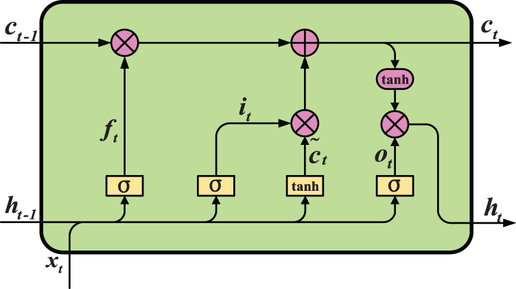
Figure 1: Illustration of the structure of the LSTM unit [21]

The forgetting gate ft can control long-term information data. The input values of the forgetting gate are the outputs of the traffic flow sequence data ht−1 and the real-time traffic flow data xt at the previous moment. The inputs need to be processed by the weight matrix of the forget gate Wf and the bias term of the forgetting gate bf and to be controlled by a σ function (sigmoid function). The σ function (the sigmoid function) controls the movement of the information obtained at the previous moment, and the degree of information retention is determined by a value in the range of [0,1]. The process of the forgetting gate can be expressed by

ft=σ(Wf ⋅ [ht−1, xt]+bf). (1)

The input gate it determines the information update of the traffic flow sequence data ht−1 and traffic flow data xt in the LSTM unit ct . The information processing process of the input door can be obtained as follows:

it=σ(Wi ⋅ [ht−1, xt]+bi), (2)

c~t=tanh⁡(Wc ⋅ [ht−1, xt]+bc), (3)

ct=ft∗ct−1+it∗c~t. (4)

where Wi represents the weight matrices of the input gate, bi and bc are the corresponding deviation vectors, c~t is the unit status update value at time t , Wc represents the weight matrices of the input unit, it is the input gate, ct−1 is the unit status value at time t−1 , and ct is the unit status value at time t .

The output gate ot can directly determine the output information ht in the current state of the LSTM neural network ct . The information processing process of the output gate can be expressed by the following formula:

ot=σ(Wo ⋅ [ht−1, xt]+bo), (5)

ht=ot∗tanh⁡(ct), (6)

where Wo is the weight matrix of the output gate, and bo is the corresponding deviation vector.

3.2 GCN Model

The spatial relationship of the road network has a non-European graphic structure, which can be abstracted as a directed graph structure. Every intersection or road section can be regarded as a node. A graph convolutional network (GCN) is suitable for extracting the data features of the non-Euclidean structure. Therefore, a GCN can be employed to capture the spatial characteristics of traffic flow data when predicting traffic flow [30]. The GCN model consists of three parts: the input layer, the hidden layer, and the output layer. First, the traffic network topology graph is entered through the input layer of the GCN model, and the data are transmitted to the convolution layer in the hidden layer. Then the graph convolution operator sequentially traverses all nodes in the topology graph for convolution operations, and the global features of the topology graph are obtained with multi-layer convolution operations. The structure of the GCN neural network model is shown in Fig. 2.

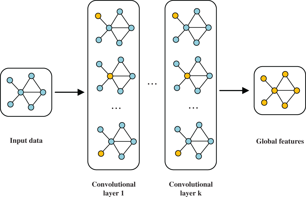
Figure 2: Graph convolution network structure [31]

The convolution operations in the GCN model are mainly divided into two categories: spatial graph convolution and frequency graph convolution. Spatial graph convolution is a convolution operation that is defined directly based on the spatial adjacency matrix, including two processes of passing information and updating the state. The spatial graph convolution framework can be obtained:

hvl+1=Ul+1(hv, ∑Ml+1(hvl, hul, xuv)), (7)

where u and v represent nodes, hvl represents the graph convolution characteristics of node v at layer l , hul represents the graph convolution characteristics of node u at layer l , xuv represents the node characteristics, hvl+1 represents the graph convolution feature information of node v at layer l+1 , and Ml+1 and Ul+1 are aggregate functions.

Frequency domain convolution is the convolution operation using the Fourier transform of the graph. The Laplacian matrix L=Dv−A can be expressed as L=In−Dv−12ADv−12 after normalization. The Laplacian matrix L is a positive semi-definite real symmetric matrix, and the feature can be decomposed into L=UΛUT . Similar to the convolution operation in Euclidean space, the convolution operation can be expressed as x∗g=U(UTx ⊙ UTg)=U(UTg ⊙ UTx) . Taking UTg as the trainable graph convolution kernel gθ , the graph convolution operation can be simplified as follows:

x∗g=UgθUTx, (8)

where x represents the input signal, g is the convolution kernel, gθ is the trainable convolution kernel, In is the identity matrix, A is the adjacency matrix, Dv is the node degree matrix, Λ is the diagonal matrix composed of the corresponding eigenvalues, U is the feature vector, ⊙ is the Hadamard product, ∗ represents the convolution operation, and UTx is the graph Fourier transform.

To speed up the calculation of the eigenvalues and eigenvectors of the Laplace matrix and reduce the calculation cost, the order Chebyshev network is used to approximate the convolution kernel of spatial map convolution. Instead of the convolution kernel, the Chebyshev polynomial can be obtained:

gθ(Λ)=∑k=0k−1θkTk(Λ~), (9)

where Λ~ is the normalized eigenvalue diagonal matrix, Tk(Λ~) is the k -order Chebyshev polynomial of Λ~ , θk is the corresponding coefficient vector, which is the parameter updated iteratively in the model training, Λ~=2Λ/2Λλmaxλmax−In , λmax represents the maximum characteristic value, and the input value of the Chebyshev polynomial is standardized to be between [−1, 1] . At this time, the plot volume operation can be expressed as follows:

x∗gθ=U(∑i=1KθiTk(Λ~))UTx=∑i=1KθiTk(UΛ~UT)x=∑i=1KθiTk(L~)x, (10)

where Tk(L~)=2L~Tk−1(L~)−Tk−2(L~) , T0(L~)=1 , T1(L~)=L~ , and L~=2L/2Lλmaxλmax−In .

Therefore, when k=1 and the maximum eigenvalue λmax=2 , L~=L−In , and the graph convolution calculation can be expressed as follows:

x∗gθ≈θ0x−θ1(L−In)x=θ0x−θ1D−12AD−12x, (11)

where L~ is the normalized eigenvalue Laplace matrix; θ0 and θ1 are the learning parameters of the graph. To avoid overfitting, assuming that θ=θ0=−θ1 , the graph convolution calculation can be given as follows:

x∗gθ≈θ(In+D−12AD−12)x. (12)

At this point, the first-order Chebyshev network is renormalized to avoid problems such as gradient explosion and numerical instability, so D~−12A~D~−12=In+D−12AD−12 , A~=A+In , D~ii=∑jA~ij . Then the graph convolution of the first-order Chebyshev network can be obtained as follows:

hl+1=f(hl, A)=σ(D~−12A~D~−12hlWl), (13)

where D~ represents the angle matrix, A~ represents the adjacency matrix with a self-ring, D~ii represents the element on the diagonal of the matrix, A~ij represents the element of the adjacency matrix, hl+1 represents the graph convolution feature of layer l+1 , hl represents the graph convolution feature of layer l , Wl represents the weight matrix of layer l , and σ represents a sigmoid activation function.

3.3 Problem Description

In traffic flow prediction, it is necessary to transform the topological structure of an urban road network into a spatiotemporal traffic map and then predict the traffic flow data in multiple time intervals (T) in the future through the prediction model function. Taking the intersection as the node in the road network diagram and the road section as the edge in the road network diagram, the traffic diagram G=f(V, E, W, t) is constructed. The traffic flow prediction problem can be expressed as follows:

[Xt−T+1, ⋯, Xt; G] ⟶f(⋅) [Xt+1, ⋯, Xt+T], (14)

where V represents the collection of intersections, E represents the collection of sections, W represents the connectivity between nodes at time t , that is, the weight matrix of the edges, and X represents the traffic flow prediction data at the corresponding time.

Assuming that there are N nodes in the traffic graph G , the directed graph of the traffic network can be represented by the adjacency matrix A :

A=[A11⋯AN1⋮⋱⋮A1N⋯ANN], (15)

Aij={ 0      Vij ∉ E 1       Vij∈E, (16)

where Aij represents the element of the adjacency matrix, and Vij represents the connecting section from intersection i to intersection j . Additionally, when Aij=0 , Vij reflects the fact that intersection i and intersection j are not directly connected. When Aij=1 , Vij indicates that there is a direct connection between intersection i and intersection j .

4  GCN-LSTM Flow Direction Level Traffic Flow Prediction Model Construction

In the process of building the model, the historical traffic flow data need to be put into the model, and the GCN network is used to extract the spatial characteristics among the data. Then the LSTM neural network is used to extract the time series characteristics of the data. Next, the retained information, discarded information, and updated information for the data in the prediction model are determined by the LSTM neural network. Finally, based on the historical information, the traffic flow parameters are predicted to determine the output information. The algorithm structure of the GCN-LSTM flow direction level traffic flow prediction model based on spatiotemporal characteristics is shown in Fig. 3.

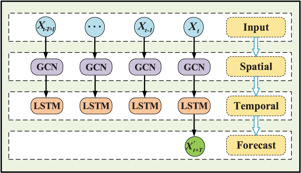
Figure 3: GCN-LSTM flow direction level traffic flow prediction model structure

To show the relationship between the GCN model and the LSTM model in detail, the connection between the GCN spatial structure convolution layer and the LSTM time series prediction layer is demonstrated in Fig. 4. The connection sequence is as follows. First, the traffic flow sequence data ht−1 and the unit information state ct−1 at time t−2 are produced by the LSTM unit structure, and then the sequence data ht−1 and the traffic flow data xt at time t form the new sequence data [ht−1, xt] . Using [ht−1, xt] , the data for ht−1′ are obtained through the first convolution structure of the GCN model, and the data for ht−1′′ are received through the second convolution structure. After this, the sequence data for ht−1′′ and the unit information state ct−1 enter the next LSTM unit structure, and the output data at time t−1 are obtained through the input gate, forgetting gate, and output gate of the LSTM unit structure. The specific output data are the updated sequence data ht and information state ct that are stored at time t−1 of the LSTM model, as well as the traffic prediction data x′t . After completing the above steps, the prediction of the next time series starts running until the prediction time interval ends.

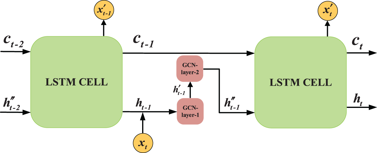
Figure 4: Connection diagram between spatial structure convolution layer and time series prediction layer

In the case of constructing the dynamic traffic association diagram G , it is assumed that the section inflow between intersections is equal to the section outflow. Considering the dependence between the weight of nodes and the flow of the intersections, the weight is expressed by the correlation degree between nodes. The higher the correlation degree is, the greater the weight value is. In the specific modeling process, the correlation degree between intersections is classified into the static correlation degree and the dynamic correlation degree. The dynamic correlation degree refers to the proportion of the flow direction of the traffic flow at the two intersections. The static correlation degree refers to the relationship regarding the distance between the intersections, road parameters, and other indicators.

The dynamic correlation degree p~ij of graph G in [t, t+1] time is the proportion of the traffic flow qij from intersection i to intersection j relative to the total flow of intersection i , that is, the flow diversion probability from intersection i to intersection j . For the weight calculation of the first-order adjacency matrix, qij includes the sum of the traffic flow of going straight, turning left, and turning right from intersection i to intersection j , and at any [t, t+1] time, ∑p~i=1 . Then the intersection dynamic correlation degree is obtained with

p~ij=∑tt+1qij∑tt+1Qi=∑tt+1(qijl+qijs+qijr)∑tt+1Qi. (17)

In the formula, qijl , qijs , and qijr represent the traffic flow from intersection i to intersection j by turning left, going straight, and turning right, respectively; Qi represents the total flow of intersection i .

To simplify the model structure and improve the operation efficiency, the static correlation degree between intersections is expressed by the intersection spacing, and its impact on the model performance is explored. In addition, the geometric parameters of different sections in the same road are similar, so the influence of the road parameter is removed in the subsequent modeling. Based on the above assumptions, the static correlation degree considering intersection spacing and correction parameters is given as follows:

spij=dij+r1∑(qij−q¯ij)2, (18)

where dij represents the distance from intersection i to intersection j , and r1 represents the coefficient of the correction distance.

Combining the static correlation degree, the dynamic correlation degree, and the traffic flow data at the corresponding time, the weight matrix of the traffic map can be obtained. The corresponding elements of the matrix are multiplied to obtain the graph convolution operator GCNt of layer l in the GCN-LSTM combined neural network model. The specific expression is

GCNtl=(Wtl⊗sp⊗p~) ⋅ xt, (19)

where Wt represents the weight matrix, ⊗ represents the multiplication of the corresponding elements of the matrix, and xt represents the traffic parameter data at time t .

At this point, the GCN-LSTM combined neural network model has been built. Using this model to predict traffic flow, the forgetting gate, input gate, output gate, and input unit state of the model at time t can be calculated with the following formula:

{ft=σ(Wf ⋅ GCNt+Uf[ht−1, xt]+bf)it=σ(Wi ⋅ GCNt+Ui[ht−1, xt]+bi)c~t=tanh⁡(Wc ⋅ GCNt+Uc[ht−1, xt]+bc)ot=σ(Wo ⋅ GCNt+Uo[ht−1, xt]+bo)ct=ft∗ct−1+it∗c~tht=ot∗tanh⁡(ct), (20)

where Uf , Ui , Uo , and Uc are the weight matrices of the previously hidden layer.

In the case of illustrating the modeling process clearly, the framework of the proposed GCN-LSTM flow direction level traffic flow prediction model is created, as shown in Fig. 5.

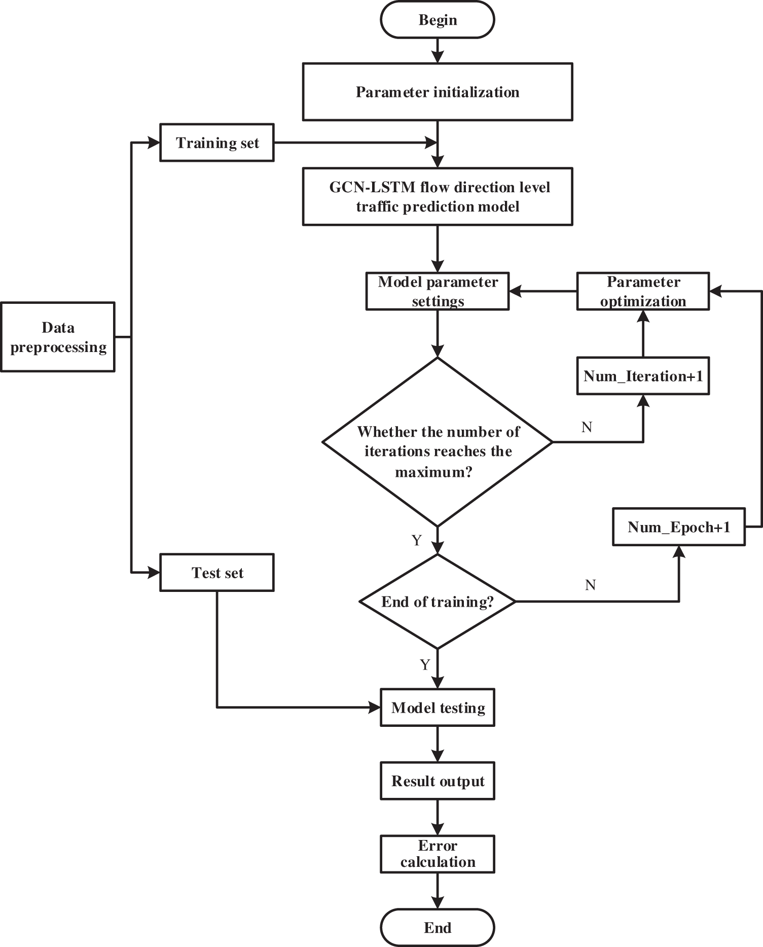
Figure 5: Framework of the proposed GCN-LSTM flow direction level traffic flow prediction model

5  Experiment and Analysis

5.1 Dataset

In this study, the north approach of the intersection of Liuquan Road and Zhongrun Avenue is selected as the experimental site in the Zibo High-Tech Zone of China. A road network topology is provided around the target intersection. The positions of the sensors and the traffic flow in the relevant direction are shown in Fig. 6. The topology diagram is provided to show the spatiotemporal dependence pattern of the network traffic. Data collection is conducted with a time interval of two hours, during the morning peak (6:30–8:30), evening peak (16:30–18:30), and off-peak (13:00–15:00) periods, in 66 working days in April, May, and June 2022. Taking the morning peak as an example, the data are aggregated at intervals of 5, 10, 15, and 20 min, and 1584 data groups, 792 data groups, 528 data groups, and 396 data groups are obtained, respectively. The traffic flow prediction models are established successively based on GCN-LSTM, GCN, LSTM, and ARIMA-LSTM. The prediction performance of each model is analyzed, based on various time intervals in different periods. Additionally, the prediction ability of the traffic flow prediction model is verified according to the data in different periods. To improve the training effect of the model, make the gradient drop rapidly, and accelerate the convergence of the model, the data values are mapped to [0,1] using min−max standardization processing, as shown in the following equation:

Figure 6: Road network topology

y′=y−min(y)max(y)−min(y), (21)

where y′ represents a scalar value, y represents the original data, max(y) represents the maximum value of the original data, and min(y) is the minimum value of the original data.

5.2 Parameter Setting

To quantitatively compare the prediction performances of the proposed model and the other models, the root mean square error (RMSE), mean absolute error (MAE), and accuracy (ACC) are used as indicators to evaluate the prediction performance [32,33].

(1) RMSE

RMSE=1N∑t=1N(y^t−yt)2. (22)

(2) MAE

MAE=1N∑t=1N|y^t−yt|. (23)

(3) ACC

ACC=(1−1N∑t=1N|y^t−ytyt|)×100%. (24)

In Eqs. (22)–(24), N is the number of data samples, yt is the measured data value at time t, and y^t is the predicted value.

Considering the influence of the signal timing scheme on the traffic flow combination, the prediction performances of the GCN-LSTM combined model, the ARIMA-LSTM combined model, the GCN model, and the LSTM single model are compared for different periods. Additionally, the flow direction level traffic flow is predicted based on the optimum period. Finally, the maximum number of iterations is 1000, and the learning rate is 0.01. The flow data are divided into a training set and a testing set with a ratio of 10:1. By slightly increasing the number of hidden layers and the number of hidden layer neurons, the errors can be effectively reduced, and the accuracy can be improved. However, it should be noted that too many layers lead to more complex networks. Comparisons of the prediction results for the GCN-LSTM combined model for different hidden layers and a different number of neurons are shown in Tables 1 and 2.

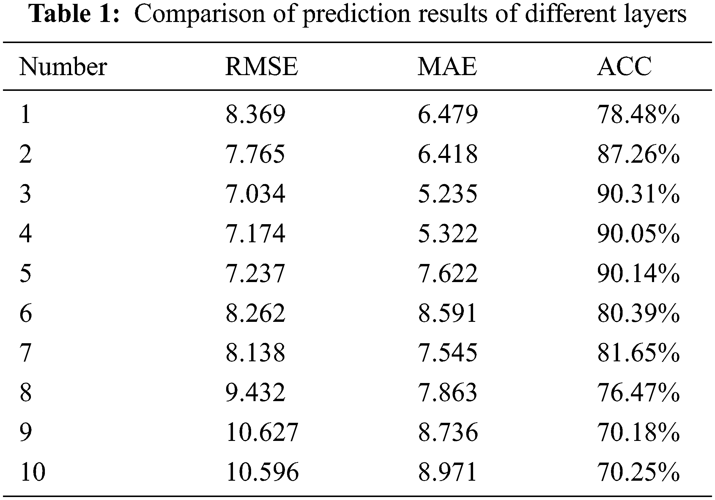
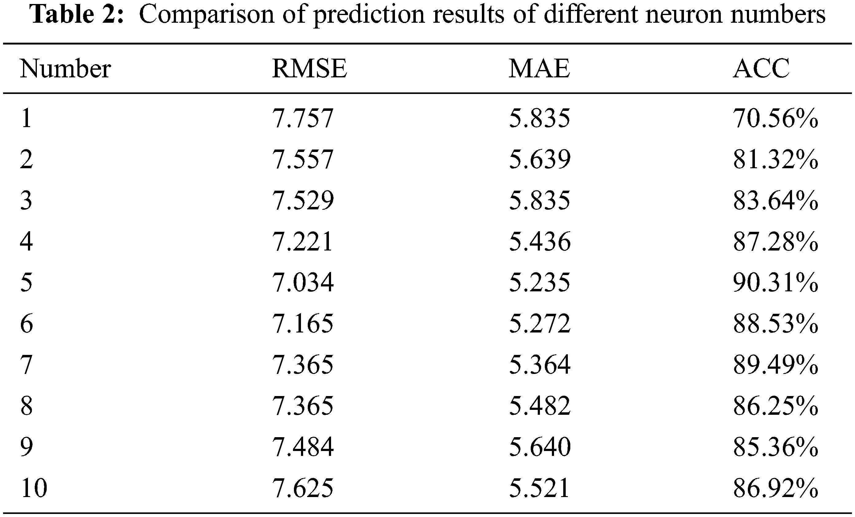
The results show that the prediction accuracy reaches the highest value when the number of hidden layers of the model is three. At this time, when the number of neurons is five, the corresponding prediction effect is the best. For the order k of the Chebyshev polynomial, the larger the value of k is, the wider the captured spatial structure is. However, at the same time, the increase in the value of k also increases the complexity of model learning and reduces the performance of the model. Through the comparative experiments for different orders, when the order is equal to three, the model has the best performance.

5.3 Analysis of Experimental Results

The prediction performance of each prediction model at different time intervals is shown in Table 3. It can be observed in Table 3 that the four traffic flow prediction models have smaller error at the 5 min time interval than the others. Compared to the existing models, the developed GCN-LSTM combined prediction model integrates the temporal and spatial characteristics to achieve higher predictive accuracy. Because residents are more likely to travel in the peak period and the traffic volume in the off-peak period appears to be more dispersed and fluctuated, the GCN-LSTM combined prediction model performs better in the peak period than in the off-peak period. The model produces better results in the late peak period than in the early peak period since the period is larger at the late peak than at the early peak.

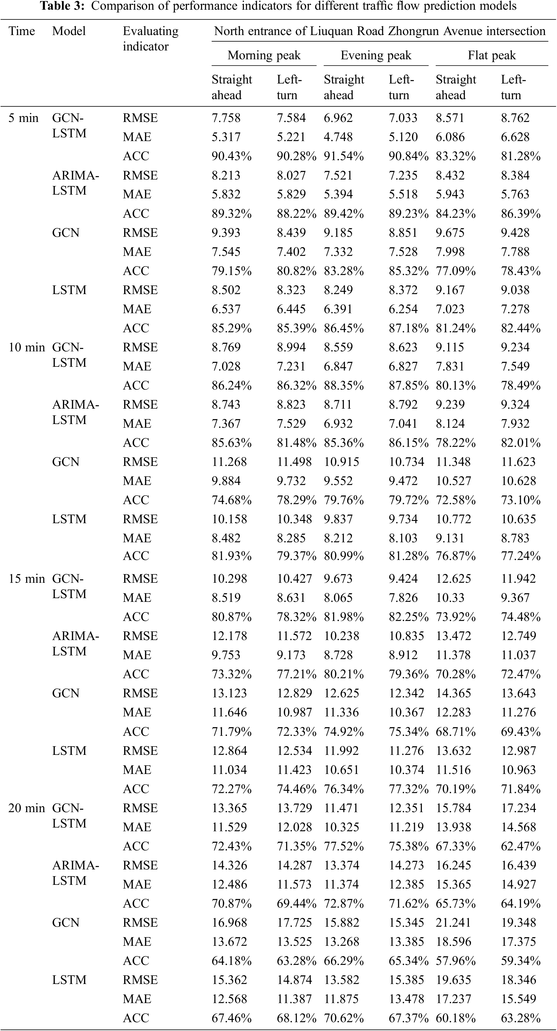
When the periods of the early peak and late peak are the same, the fluctuation of the traffic flow is slightly smaller in the late peak than that in the early peak. Taking the evening peak as an example, the ARIMA-LSTM combined prediction model is compared with the second best one, which is the GCN-LSTM combined prediction model at the time interval of 5 min. The RMSE of straight travel is reduced by 7.43%, the MAE is reduced by 11.98%, and the ACC is increased by 2.37%. The left-turn RMSE is decreased by 2.79%, the MAE is decreased by 7.21%, and the ACC is increased by 1.80%.

The north entrance of the intersection of Liuquan Road and Zhongrun Avenue on the last working day of June is chosen for the verification of the traffic flow. The flows are divided into going straight and turning left according to their directions and are aggregated at the interval of 5 minute. Additionally, the GCN-LSTM model is used to verify the prediction effect of the flow level for each direction. Next, five minutes is selected as the prediction time interval, and the GCN-LSTM prediction model is used to predict the flow direction of the through and left-turn traffic flows. The prediction results for the through and left-turn flow directions are shown in Figs. 7 and 8, respectively. The figures show the comparisons between the predicted values and the real values of the traffic flow in different directions in the morning peak and the evening peak, as well as the fluctuations of the prediction error.

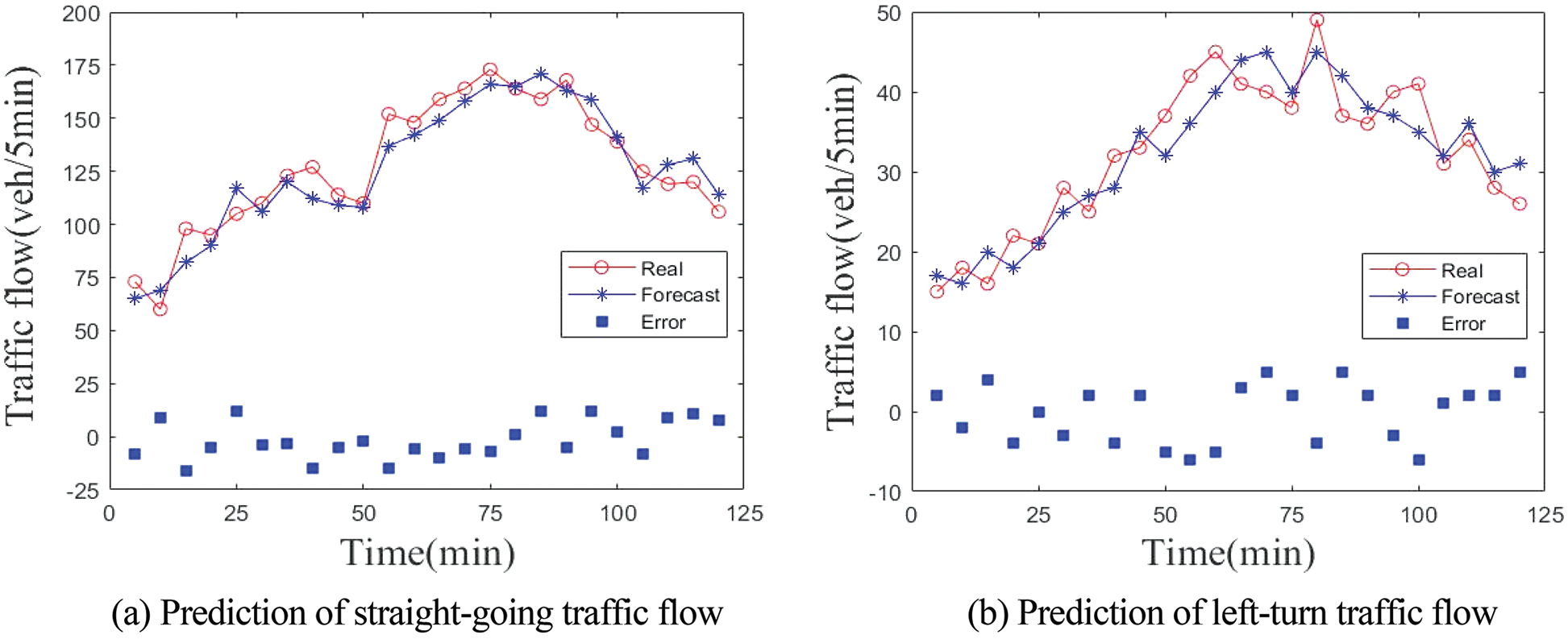
Figure 7: Traffic flow prediction of morning peak

Figure 8: Traffic flow prediction of evening peak

It can be seen in Figs. 7 and 8 that the predicted values of the GCN-LSTM model for traffic flow are consistent with the actual values in general, and the predicted values are much closer to the actual values during the morning peak and evening peak hours.

6  Conclusions

To identify the spatiotemporal characteristics of road traffic flow, the GCN-LSTM flow direction level traffic flow prediction model based on spatiotemporal characteristics is proposed to capture the spatiotemporal characteristics in this study. Through the model verification, the developed GCN-LSTM combined flow direction level traffic flow prediction model performs better in predicting traffic flow than the GCN, the LSTM single prediction model, and the ARIMA-LSTM combined prediction model. In the proposed model, the high-dimensional time characteristics of traffic flow data are obtained through the LSTM network. The adjacent matrix of the GCN model is integrated to describe the relationship between the nodes of the road network. The spatial distribution characteristics of different periods of traffic data are obtained by mining the space-time correlation of traffic flow in different directions. In this study, the proposed model can be applied to predict the flow direction level traffic flow at intersections and to obtain more accurate traffic volume information.

In the next step, the flow direction level predictions can be applied to the field of information control to forecast the traffic flow in different directions at each entrance of an intersection. The parameters obtained in this study can help traffic engineers to design the intersection signal timing, to improve the fitting degree between the signal timing parameters and the traffic operation conditions, and to further improve road traffic efficiency and safety. This provides method support for the refined, intelligent, and dynamic management and control of signalized intersections.

Flow direction level traffic flow prediction also faces a series of challenges. For example, hardware support with full coverage of license plate recognition data in the flow direction level is required. The implementation effect of the prediction method is reduced by the low flow detection accuracy of the signal management and control platform.

Acknowledgement: The authors appreciate the support of the Shandong Department of Transportation (SDOT), the Zibo Department of Transportation (ZDOT), and the Center for Accident Research in Zibo (CARZ). We thank LetPub (www.letpub.com) for its linguistic assistance during the preparation of this manuscript.

Funding Statement:: This research was jointly supported by the National Natural Science Foundation of China (Grant Nos. 71901134 & 51878165) and the National Science Foundation for Distinguished Young Scholars (Grant No. 51925801).

Conflicts of Interest:: The authors declare that they have no conflicts of interest to report regarding the present study.

References

1. M. S. Roopa, S. A. Siddiq, R. Buyya, K. R. Venugopal, S. S. Iyengar et al., “DTCMS: Dynamic traffic congestion management in Social Internet of Vehicles (SIoV),” Internet of Things, vol. 16, no. 2, pp. 100311, 2020. [Google Scholar]

2. D. F. Ma, J. W. Xiao, X. Song, X. L. Ma and S. Jin, “A back-pressure-based model with fixed phase sequences for traffic signal optimization under oversaturated networks,” IEEE Transactions on Intelligent Transportation Systems, vol. 22, no. 9, pp. 5577–5588, 2021. [Google Scholar]

3. F. L. Wei, Z. G. Cai, Y. Q. Guo, P. Liu, Z. Y. Wang et al., “Analysis of roadside accident severity on rural and urban roadways,” Intelligent Automation & Soft Computing, vol. 28, no. 3, pp. 753–767, 2021. [Google Scholar]

4. D. F. Ma, X. B. Song, J. C. Zhu and W. H. Ma, “Input data selection for daily traffic flow forecasting through contextual mining and intra-day pattern recognition,” Expert Systems with Applications, vol. 176, no. 6, pp. 114902, 2021. [Google Scholar]

5. X. Q. Luo, D. H. Wang, D. F. Ma and S. Jin, “Grouped travel time estimation in signalized arterials using point-to-point detectors,” Transportation Research Part B: Methodological, vol. 130, no. 3, pp. 130–151, 2019. [Google Scholar]

6. M. Gohar, M. Muzammal and A. U. Rahman, “SMART TSS: Defining transportation system behavior using big data analytics in smart cities,” Sustainable Cities and Society, vol. 41, no. 2, pp. 114–119, 2018. [Google Scholar]

7. D. F. Ma, X. M. Song and P. Li, “Daily traffic flow forecasting through a contextual convolutional recurrent neural network modeling inter-and intra-day traffic patterns,” IEEE Transactions on Intelligent Transportation Systems, vol. 22, no. 5, pp. 2627–2636, 2021. [Google Scholar]

8. L. R. Cai, Z. C. Zhang, J. J. Yang, Y. D. Yu, T. Zhou et al., “A noise-immune kalman filter for short-term traffic flow forecasting,” Physica A, vol. 536, no. 1, pp. 122601, 2019. [Google Scholar]

9. Y. R. Ning, H. Kazemi and P. Tahmasebi, “A comparative machine learning study for time series oil production forecasting: ARIMA, LSTM, and Prophet,” Computers and Geosciences, vol. 164, no. 1, pp. 105126, 2022. [Google Scholar]

10. J. S. Ou, X. M. Huang, Y. Zhou, Z. G. Zhou and Q. H. Nie, “Traffic volatility forecasting using an omnibus family GARCH modeling framework,” Entropy, vol. 24, no. 10, pp. 1392, 2022. [Google Scholar]

11. H. Yan, T. A. Zhang, Y. Qi and D. J. Yu, “Short-term traffic flow prediction based on a hybrid optimization algorithm,” Applied Mathematical Modelling, vol. 102, pp. 385–404, 2022. [Google Scholar]

12. N. R. Ramchanfra and C. Rajabhushanam, “Machine learning algorithms performance evaluation in traffic flow prediction,” Materials Today: Proceedings, vol. 51, pp. 1046–1050, 2022. [Google Scholar]

13. J. S. Ou, J. X. Xia, Y. J. Wu and W. M. Rao, “Short-term traffic flow forecasting for urban roads using data-driven feature selection strategy and bias-corrected random forests,” Transportation Research Record: Journal of the Transportation Research Board, vol. 2645, no. 1, pp. 157–167, 2017. [Google Scholar]

14. Z. b. Lu, J. X. Xia, W. M., Q. H. Nie and J. S. Ou, “Short-term traffic flow forecasting via multi-regime modeling and ensemble learning,” Applied Sciences, vol. 10, no. 1, pp. 356, 2020. [Google Scholar]

15. J. L. Xiao, “SVM and KNN ensemble learning for traffic incident detection,” Physica A, vol. 517, no. 2324, pp. 29–35, 2019. [Google Scholar]

16. J. Wang, W. Deng and Y. T. Guo, “New bayesian combination method for short-term traffic flow forecasting,” Transportation Research Part C, vol. 43, no. 7, pp. 79–94, 2014. [Google Scholar]

17. T. Bogaerts, A. D. Masegosa, J. S. Angarita-Zapata, E. Onieva and P. Hellinckx, “A graph CNN-LSTM neural network for short and long-term traffic forecasting based on trajectory data,” Transportation Research Part C, vol. 112, pp. 62–77, 2020. [Google Scholar]

18. W. B. Zhang, Y. H. Yu, Y. Qi, F. Shu and Y. H. Wang, “Short-term traffic flow prediction based on spatio-temporal analysis and CNN deep learning,” Transportmetrica A: Transport Science, vol. 15, no. 2, pp. 1688–1711, 2019. [Google Scholar]

19. Y. Q. Zhu, J. S. Ou, G. Chen and H. P. Yu, “An approach for dynamic weighting ensemble classifiers based on cross validation,” Journal of Computational Information Systems, vol. 6, no. 1, pp. 297–305, 2010. [Google Scholar]

20. Y. Q. Zhu, J. S. Ou, G. Chen and H. P. Yu, “Dynamic weighting ensemble classifiers based on cross-validation,” Neural Computing and Applications, vol. 20, no. 3, pp. 309–317, 2011. [Google Scholar]

21. S. Q. Lu, Q. Y. Zhang, G. S. Chen and D. W. Seng, “A combined method for short-term traffic flow prediction based on recurrent neural network,” Alexandria Engineering Journal, vol. 60, no. 1, pp. 87–94, 2021. [Google Scholar]

22. X. C. Xu, X. F. Jin, D. Q. Xiao, C. X. Ma and S. C. Wong, “A hybrid autoregressive fractionally integrated moving average and nonlinear autoregressive neural network model for short-term traffic flow prediction,” Journal of Intelligent Transportation Systems, vol. 26, no. 2, pp. 1–18, 2021. [Google Scholar]

23. W. D. Du, Q. Y. Zhang, Y. P. Chen and Z. L. Ye, “An urban short-term traffic flow prediction model based on wavelet neural network with improved whale optimization algorithm,” Sustainable Cities and Society, vol. 69, no. 3, pp. 102858, 2021. [Google Scholar]

24. Y. Liu, Y. L. Song, Y. Zhang and Z. F. Liao, “WT-2DCNN: A convolutional neural network traffic flow prediction model based on wavelet reconstruction,” Physica A, vol. 603, pp. 127817, 2022. [Google Scholar]

25. Z. Y. Cui, R. M. Ke, Z. Y. Pu, X. L. Ma and Y. H. Wang, “Learning traffic as a graph: A gated graph wavelet recurrent neural network for network-scale traffic prediction,” Transportation Research Part C, vol. 115, pp. 102620, 2020. [Google Scholar]

26. Y. F. Liu, C. Z. Wu, J. H. Wen, X. P. Xiao and Z. J. Chen, “A grey convolutional neural network model for traffic flow prediction under traffic accidents,” Neurocomputing, vol. 500, pp. 761–775, 2022. [Google Scholar]

27. K. Lee and W. Rhee, “DDP-GCN: Multi-graph convolutional network for spatiotemporal traffic forecasting,” Transportation Research Part C, vol. 134, no. 4, pp. 103466, 2022. [Google Scholar]

28. X. X. Ta, Z. H. Liu, X. Hu, L. Yu, L. L. Sun et al., “Adaptive spatio-temporal graph neural network for traffic forecasting,” Knowledge-Based Systems, vol. 242, pp. 108199, 2022. [Google Scholar]

29. J. M. Yang, Z. R. Peng and L. Lin, “Real-time spatiotemporal prediction and imputation of traffic status based on LSTM and Graph Laplacian regularized matrix factorization,” Transportation Research Part C, vol. 129, no. 8, pp. 103228, 2021. [Google Scholar]

30. J. H. Ye, S. J. Xue and A. W. Jiang, “Attention-based spatio-temporal graph convolutional network considering external factors for multi-step traffic flow prediction,” Digital Communications and Networks, vol. 8, no. 3, pp. 343–350, 2022. [Google Scholar]

31. D. Y. Huang, H. Liu, T. S. Bi and Q. X. Yang, “GCN-LSTM spatiotemporal-network-based method for post-disturbance frequency prediction of power systems,” Global Energy Interconnection, vol. 5, no. 1, pp. 96–107, 2022. [Google Scholar]

32. Z. G. Shen, W. L. Wang, Q. Shen, S. J. Zhu, H. M. Fardoun et al., “A novel learning method for multi-intersections aware traffic flow forecasting,” Neurocomputing, vol. 398, no. 4, pp. 477–484, 2020. [Google Scholar]

33. X. Han, G. J. Shen, X. Yang and X. J. Kong, “Congestion recognition for hybrid urban road systems via digraph convolutional network,” Transportation Research Part C, vol. 121, no. 5, pp. 102877, 2020. [Google Scholar]