Circular Formation Control with Collision Avoidance Based on Probabilistic Position

1  Introduction

Owing to the current technological development/progress in computation and communication, distributed cooperative control of multi-agent systems (MASs) has received enormous attention from research communities in recent years. Its practical applications include search mechanisms, navigation, map manipulation, target interception, and tracking [1–4]. The main objective of cooperative control theory is to develop and design a protocol that guarantees the synchronization of a group of neighboring agents via local information exchange. Literature studies present different phenomena in cooperative control, such as consensus [5,6], formation control [7], and containment control [8].

Formation control is one of the fundamental research problems in distributed cooperative control of MASs that has presented wide application prospects, such as unmanned aerial vehicles (UAVs) [9], unmanned ground vehicles (UGVs) [10], autonomous underwater vehicles (AUVs) [11], coordination control of satellites [12], etc. In general, formation control aims to design a distributed control protocol that leads the state/output of the agent to maintain an expected shape. The formation control problem has been investigated using different control techniques in recent years. Based on [13], the techniques are classified into three strategies, namely, distance-based [14], displacement-based [15], and bearing-based [16] strategies. The consensus-based techniques are used to address the formation control problems in [17,18]. In [19], the adaptive control design is introduced to address the formation tracking problem of multiple mobile robots with unknown skidding and slipping environments. The distributed formation control problems are addressed in [20] by using an event-triggered mechanism. Based on multiple Euler-Lagrange functions, the authors in [21] investigated formation control design. In [22], a novel fault-tolerant control strategy is developed by utilizing decentralized state observers for multi-quadrotor systems. Based on the leader-follower method, a distributed adaptive-based sliding mode formation control scheme is designed for a class of second-order nonlinear MASs with unknown dynamics [23].

Among the challenging problems proposed in the formation control of MASs, the circular formation becomes a hot subject of interest because of its manifold applications, such as source-seeking exploration [24], surveillance [25], and sensor networks [26]. Circular formation control is to drive a group of agents to converge to or move on a defined circular trajectory with spacing adjustment between the neighboring agents [27]. Up to now, scholars are progressively adopting innovative research strategies and measurements to investigate the circular formation control problem of MASs. Several methodologies have been proposed to deal with the circular formation control problem, including the leader-follower technique [28], the cyclic pursuit technique [29], the behavioral technique [30], and the virtual structure technique [31]. In [32], authors developed a circular motion control law and phase-distributed protocol to achieve a circular formation for any preset relative phase. In [33,34], distributed control protocols are designed to solve the circle-forming problem of a group of anonymous agents. The circular formation stabilization of networked dynamic unicycles is considered in [35], where a distributed dynamic protocol is developed for each unicycle. Interested readers are referred to the survey paper [36] for a comprehensive review of the techniques and methodologies in circular formation control of MASs.

From a practical perspective, collision avoidance is one of the fundamental and challenging problems in formation control. A collision avoidance strategy is developed for multiple UAVs in formation flight to avoid collisions and obstacles [37]. In [38], formation tracking control with collision avoidance problem is addressed for nonlinear MASs by adopting the artificial potential approach with the neural networks technique. A novel control scheme based on adaptive neural networks is designed for a class of second-order nonlinear MASs to solve the formation control problem with multiple tasks, including obstacle avoidance, collision avoidance, and connectivity maintenance [39].

Although considerable research efforts devoted to the circular formation control problem, most of the existing results consider the single-integrator model [28,33,40], and only a few works have considered collision avoidance. Thus, it is of practical significance to study more realistic models, such as models that capture UAV systems. In this work, the circular formation problem has a wide array of practical potential applications in engineering. It has applications in the defense industry to provide surveillance and navigation of a particular area within a defined radius. It has applications in escorting and patrolling tasks of multi-robots, such as UAVs patrolling borders [41]. These facts motivate us to develop a novel distributed control scheme to achieve circular formation and meet practical challenges.

Motivated by the aforegoing observation, the problem of circular formation for the second-order MASs based on a probabilistic position is addressed in this paper. The mobile agents are required to follow a circular trajectory such that the agents in the circular trajectory must have the same direction. Compared to the existing circular formation control techniques [28,42], the leader-follower strategy and probabilistic position are combined to solve the circular formation problem, which significantly enhances the flexibility and stability of the system. The main difficulty in this paper is caused by the fact that the agents may get a tangential path after getting in a circular trajectory. By using the Lyapunov methods, convergence analysis of the designed circular formation control protocol is provided. The main contributions of this work are as follows. First, unlike [33,40], this paper considers the circular formation of second-order MASs, which makes this work more application-oriented. The second-order systems can be used to model many real systems, such as unicycle dynamics (after dynamic feedback linearization) or quadrotor UAV simplified dynamics. Second, by introducing a probabilistic position control law, a novel distributed control protocol is proposed to achieve circular formation, which is different from [43]. The probabilistic position law is proposed to represent the probabilistic position of each agent in the circular trajectory. It is shown that under the proposed control scheme the agents move along the circular trajectory of the desired radius and also avoid the tangential path. Third, the proposed control strategy guarantees inter-agent collision avoidance.

The rest of the paper is organized as follows. Section 2 represents notations and preliminaries. Section 3 formulates the circular formation problem and presents the controller design. Section 4 discusses the main results. Finally, Section 5 presents simulation results and Section 6 summarizes the conclusions of the study.

2  Notations and Preliminaries

2.1 Notations

Throughout this paper, let , , and represent the sets of nth dimensional space, real matrices, and integer numbers, respectively denotes the identity matrix of dimension . denotes the transpose of a matrix or vector M. denotes a block diagonal matrix. is the Euclidean norm of a vector x. The notation stands for the Kronecker product. The subscript represents the orbits. represents the orientation of agents such that for the clockwise direction and for the counterclockwise direction.

2.2 Graph Theory

In MASs, the interaction topology is represented by a graph [44]. A graph and an edge set . The weighted adjacency matrix of graph is given by where if and otherwise. Neighbors set of the vertex is denoted by a set . The graph is undirected if . The (weighted) graph Laplacian matrix is represented as where is the degree matrix with . A graph contains a spanning tree if there exists a node from such that there is a path to any node in the graph. A graph is strongly connected if every pair , are connected.

Definition 1 (Laplacian). The Laplacian matrix is given as where

where the adjacency matrix is defined by ,

3  Control Law Design

3.1 Problem Formulation

We consider a group of agents initially located in a plane, each agent must maintain circular formation as shown in Fig. 1. The dynamics of each agent i is defined as

(1)

where , , and represent the position, velocity, and control input of the agent to be designed, respectively.

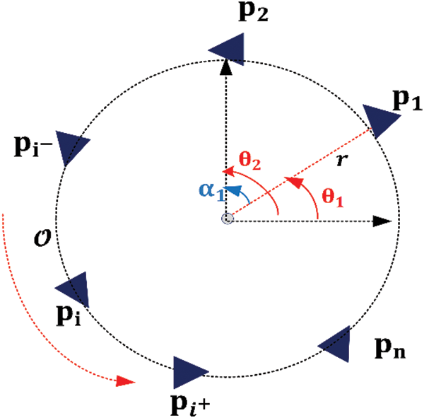
Figure 1: The desired circular formation in a counterclockwise direction, maintaining circular distance and avoiding tangential movement

Definition 2. (Circular path). The agents move in a circular formation if

(2)

For a given desired radius vector of different circular trajectories the agents maintain circular formations with different radii if

(3)

If then the agents are moving in the same circular trajectory otherwise they are in a different circular trajectory.

Definition 3. (Agents direction). The agent must have the same direction of motion but for different circular trajectories, the agent direction may be different.

Definition 4. (Collision avoidance condition). For given desired . The agents in the same circular trajectory have the property of collision avoidance if

(4)

and constant.

Definition 5. (Problem definition). For a given n such that each agent maintains the circular formation with collision avoidance.

To achieve this objective, let us assume that:

•   All the agents must move in one direction with the same constant angular velocity in the same orbit.

•   There exist a constant distance between agents to avoid collisions, the distance between agents is rotational in the same circle as well as different circles.

•   Each agent knows its initial velocities

•   The position of each agent is presumed, because of its circular trajectory.

•   The dynamics of followers (trajectory and uncertainty) are stabilizable which means that the pair is stabilizable.

3.2 Probabilistic Position

The probabilistic position law of each dynamic agent along circular trajectories modeled by the system Eq. (1) can be designed as

4  Main Results

Lemma 1. [44] Let , then

1.    

2.    If eigenvalues are positive.

Lemma 2. (Young’s Inequality, [45]). If .

Lemma 3. [46] Under a time-invariant information exchange topology, the continuous-time protocol achieves consensus asymptotically if and only if the information exchange topology has a spanning tree.

Lemma 4. Consider the multi-agent system (1). The system uncertainties are supposed as:

i.   Agents not maintaining a circular path,

ii.   Agents may get a tangential path after getting in a circular trajectory, getting a .

Proof.

i.   Agents not maintaining a circular path is a contradiction to Definition 2, which will affect formation. Let’s consider . Let’s assume that is the position of agent i and is the position of agent . If (circular path), we have because the derivative across any point/line/plane is a slope . Let’s assume the distance covered by is , then the distance covered by , which means: if is achieved it means that the consensus is achieved for i and j, and are following the same trajectory (circular).

ii.   While getting a tangential trajectory is a contradiction to Definition 2. We have , which means that the value for , implies that agent i is the leader following the circular path, and j follows the same trajectory.

Remark 1. Each dynamic agent must follow the circular trajectory in the same radius and avoid the tangential path.

Theorem 1. Consider the multi-agent system (1). The control law generated by the probabilistic position is designed as

(5)

such that will make sure that the agents remain in the same radius and avoids the tangential path where represents the probabilistic position of each agent in each circle, represents the circular orbit, and k control gain.

Proof. For the multi-agent system (1), the controller is designed as follows [6]:

in our paper, converges to a constant value it will make sure that agents are apart from each other while maintaining strong communication links. For general formation control design, we construct the Lyapunov function as

such that , where is error function as . Then, the derivative of is given by

The desired trajectory is described as follows

The error can be calculated as . We have . Thus

By solving the Lyapunov equation for any , the matrix is obtained as

The matrix P is positive semi-definite if and only if

Remark 2. Theorem 1 leads to the contradiction that only in the static case. Thus, Lemma 4 is true only for a static case. The results are extended to the dynamic case by applying the virtual leader-follower strategy in the next subsection.

4.1 Virtual Leader-Follower Strategy

In this subsection, the virtual leader-follower strategy is designed to deal with the system uncertainties where each follower agent tracks the virtual leader dynamics. A distributed hybrid control law is designed to ensure the formation control stabilization and consensus in presence of the uncertain trajectory with tracking error converging to zero.

Lemma 5. The dynamic of the virtual leader follows a desired circular trajectory defined as

(6)

where are respectively the rotation angle, angular velocity, and control input of the virtual leader given as

(7)

where to the virtual leader.

Proof. The distributed formation stabilization controller can be designed as

(8)

and the consensus controller is proposed as follows

(9)

By adding the two controllers Eqs. (8) and (9), a distributed hybrid controller is given by

which is equivalent to

(10)

For , we obtain

(11)

Eq. (11) can be also written in a vector form as

(12)

where Furthermore, for , by substituting and into Eq. (11), we obtain

(13)

Remark 3. Under the proposed control scheme, inter-agent collision avoidance is guaranteed under the following assumptions:

a)   All the agents move in a counterclockwise direction, i.e., orientation with constant velocity.

b)   There exist a positive or constant relative distance between the agents, i.e., .

Lemma 6. Consider a graph with a directed spanning tree. The consensus is reached for the multi-agent system Eq. (1) and the control law Eq. (12) with a complex polynomial of the following form

where is stable if

and

Proof. Let , , and for . We have

for . Then, it can be written as

for , we have

where J is the Jordan matrix given as

such that are complex eigenvalues. By using the Leonhard-Mikhailov theorem, the condition of spanning (directed) is true only if and for every ,

where

which completes the case for a directed spanning tree.

Remark 4. In the circular orbit, we have an infinite set of points for the tangential trajectory. Let’s define as the tangential path, for each . Thus, will no longer be the radius as the agent not following the circular path, it will be changed to , where is the tangent on any point in the circle. The tangential trajectory will vary in the interval .

From Remark 4, for every there exists which defines the signal of the actual trajectory to be followed as

(14)

for . Then, differentiating Eq. (14) yields

To show the stability of the system, consider the Lyapunov function

It is easy to check that is differentiable and positive definite. By taking the derivative of along the trajectories of the system, we obtain

(15)

by using Young’s inequality, for each and , we have

We take

Thus, for , we have which implies that is a negative definite. Consequently, for every , is asymptotically stable. Further, the system can achieve both formation stabilization with collision avoidance and consensus.

For every , we define the error . We discuss two cases.

Case 1: when We consider the following Lyapunov function candidate

Differentiating V2 yields

Case 2: when , we define the error sets as . We choose a Lyapunov function as follows

Taking the derivative of yields

by using Young’s inequality, we have

for . If , and ; we have

We conclude that the system is stable, and the error will converge to zero. We write the system Eq. (1) in generalized form as

(16)

where , , and are the state, control input, and output of agent i, respectively. and C are constant matrices with appropriate dimensions given as follows

The feedback control gain k is given by , such that P is the positive definite solution of the following algebraic Riccati inequality (ARI)

(17)

Since, is Hurwitz the pair (A, B) is controllable.

Lemma 7. Lyapunov candidate (potential function) is the error in the dynamical system Eq. (14) given as

Proof.

We have . The derivative of V along the trajectories leads to

Applying Young’s inequality, we obtain

If and , we have

The system error is given as , and its derivative is .

The system can be written as

such that , the system can be written in compact form as

Consider candidate Lyapunov function as

Calculating the derivative of V, we get

Thus, we have

for , we have , which implies that the system is globally asymptotically stable. The pair is stabilizable. Hence, the consensus is reached, i.e., .

Since the graph is connected, we have

for a connected graph to solve the Riccati equation. For to be symmetric there exists an orthogonal matrix such that .

Theorem 2. Consider the multi-agent system (1). The dynamic control law Eq. (12) under assumptions solves the circular formation control problem.

Proof. Appendix A.

Remark 5. Theorem 2 leads to a contradiction with the Assumptions proposed. Since the virtual leader velocity may not be constant (changing velocity) the agents may maintain circular trajectories but with weak collision avoidance between interacting agents.

4.2 An Extension to Lasalle’s Invariance Principle

In this subsection, the results are extended to LaSalle’s invariance principle due to the limitations of the virtual leader-follower strategy Theorem 2. Consider a function , for , we have , these function limits can be divided as

•   For , the function L is Lyapunov stable;

•   For , the function L is unstable.

For this Lyapunov strict function, we use the LaSalle principle. LaSalle will make sure that the function with is globally stable. For , , the function is Lyapunov stable for positive . We have negative for . We choose the Lyapunov function as where . The derivative of along the trajectories is given by

We have . Suppose that , we get

Since from algebraic Riccati equation, Q is positive definite if and only if is positive. In addition, we have

is positive for every . Thus when . The results are presented in the following Theorem.

Theorem 3. The dynamic control law solves the circular formation control problem for

Proof. We consider the following system

(18)

where the vector we have

In the same way, we get

(19)

Thus, by substituting Eq. (18) into (18), we obtain

where is the probability value.

We analyze two cases: If , it means that the follower agent follows a circular trajectory with all predefined conditions. If , it means that the follower agent is not following any agents, or the agent is not following the desired formation with necessary conditions.

Remark 6. In the current system, the probability value has a fundamental rule in making the follower agents follow the circular trajectory.

Let is a probability function. The function will always result for , for any other value is referred to as an error function

is not following the circular trajectory. Thus the system is unstable. We have to define an error threshold for . Let consider and with respect to circular trajectory. To prove that the error is not affecting the system. Consider the following Lyapunov function candidate

The function ) is differentiable and positive definite. Then, the derivative of is given by

Since , we have that . Thus, if the probability is more than then the system will remain stable. So the system should have uncertainty.

5  Simulation Results

This section presents the simulation of three agents () modeled by Eq. (1), controlled by the proposed control techniques above. The communication topology of agents is shown in Fig. 2. The system matrices are given as follows

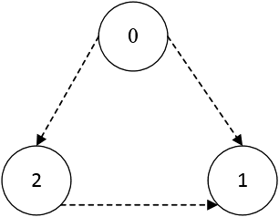
Figure 2: Graph interaction topology of two follower agents with a virtual leader in the same radius

Fig. 3 shows the trajectories of the agents uer control law (5). depicts the trajectory of the agent in the static case, where the agent follows a circular trajectory. and depict the trajectories of the agents in the dynamic case, where the agents follow tangential paths. It shows that the agents follow the desired circular trajectory in the static case. It also shows that when the agents move and change position and velocity, they may follow a tangential path or follow a circular trajectory.

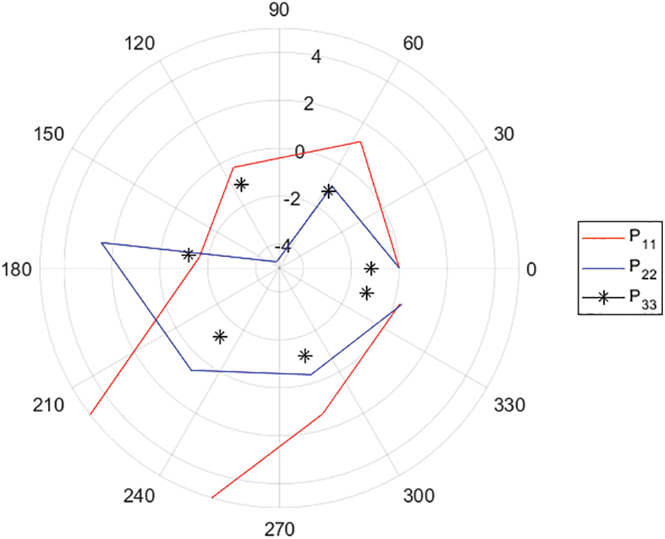
Figure 3: The trajectories of , and

Fig. 4 shows the different positions of agent i along the same circular trajectory in the plane under the proposed control protocol. It is shown that when the agent moves the tangential path is controlled but the agents can have different circular trajectories. The designed controller protocol ensures that the agents follow desired circular trajectory and avoid the tangential paths.

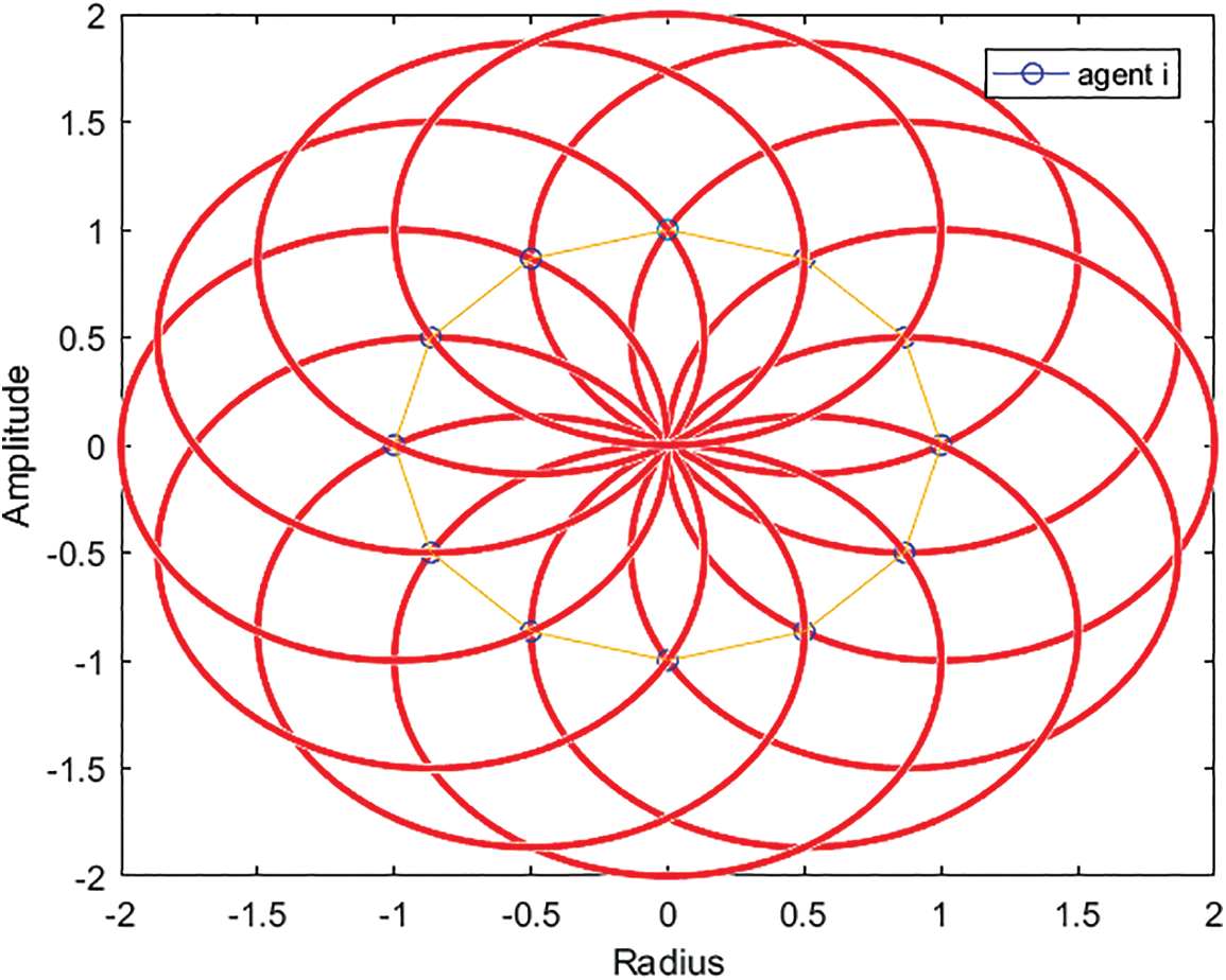
Figure 4: The different positions of the agent in the same circular trajectory under the control law

In the simulation, we consider a system consisting of three agents ( and we set the center point of the circular trajectory at (0, 0) on the plane. The initial positions of the agents are generated randomly. The design parameters are set as , demonstrated in Fig. 5. As shown in Fig. 5, the simulation results indicate that the group of mobile robots move in a counterclockwise direction to form and maintain the spaced circular formation under the proposed control law (13).

Figure 5: The circular formation trajectories of agents in the plane

The simulation results indicate clearly that the proposed control scheme solves the circular formation problem while no collision occurs among agents.

6  Conclusion

In this paper, a novel formation control scheme is introduced to study the circular formation problem for second-order MASs in the plane. The problem has two sub-objectives: circular formation control and collision avoidance. First, by combining probabilistic position law with a leader-follower strategy, a novel distributed control protocol is developed to achieve circular formation. It is proved that under the developed control scheme all the agents achieve a circular formation with the desired radius and also avoid the tangential path. Under the proposed control protocol, inter-agent collision avoidance is guaranteed by keeping the same counterclockwise direction of the agents with constant velocity and preserving a positive or constant distance between any two agents. Based on Lyapunov methods, the stability analysis of the designed circular formation scheme is provided. The effectiveness of the proposed control strategy is illustrated in the numerical simulations. Future works will focus on extending the proposed technique to MASs with more realistic dynamics. Moreover, how to achieve circular formation in different circular radii is an open and challenging research topic that needs investigation.

Funding Statement: The authors received no specific funding for this study.

Conflicts of Interest: The authors declare that they have no conflicts of interest to report regarding the present study.

References

1. R. W. Beard, T. W. McLain, M. A. Goodrich and E. P. Anderson, “Coordinated target assignment and intercept for unmanned air vehicles, ” IEEE Transactions on Robotics and Automation, vol. 18, no. 6, pp. 911–922, 2002. [Google Scholar]

2. R. W. Beard and T. W. McLain, “Multiple UAV cooperative search under collision avoidance and limited range communication constraints,” in Proc. 42nd IEEE Int. Conf. on Decis. and Control, Maui, HI, USA, pp. 25–30, 2003. [Google Scholar]

3. M. Di Marco, A. Garulli and A. Vicino, “Simultaneous localization and map building for a team of cooperating robots: A set membership approach,” IEEE Transactions on Robotics and Automation, vol. 19, no. 2, pp. 238–249, 2003. [Google Scholar]

4. T. G. Sugar and V. Kumar, “Control of cooperating mobile manipulators,” IEEE Transactions on Robotics and Automation, vol. 18, no. 1, pp. 94–103, 2002. [Google Scholar]

5. R. Olfati-Saber, J. A. Fax and R. M. Murray, “Consensus and cooperation in networked multi-agent systems,” Proceedings of the IEEE, vol. 95, no. 1, pp. 2015–233, 2007. [Google Scholar]

6. W. Ren, “On consensus algorithms for double-integrator dynamics,”IEEE Transactions on Automatic Control, vol. 53, no. 6, pp. 1503–1509, 2008. [Google Scholar]

7. X. Dong, Y. Zhou, Z. Ren and Y. Zhong, “Time-varying formation tracking for second-order multi-agent systems subjected to switching topologies with application to quadrotor formation flying,”IEEE Transactions on Industrial Electronics, vol. 64, no. 6, pp. 5014–5024, 2017. [Google Scholar]

8. J. Qin, W. X. Zheng, H. Gao, Q. Maand and W. Fu, “Containment control for second-order multiagent systems communicating over heterogeneous networks,” IEEE Transactions on Neural Networks and Learning Systems, vol. 28, no. 9, pp. 2143–2155, 2017. [Google Scholar] [PubMed]

9. Q. Li, Y. Hua, X. Dong and Z. Ren, “Time-varying formation tracking control for unmanned aerial vehicles: Theories and applications,” IFAC-PapersOnLine, vol. 55, no. 3, pp. 49–54, 2022. [Google Scholar]

10. C. Wang, H. Tnunay, Z. Zuo, B. Lennox and Z. Ding, “Fixed-time formation control of multirobot systems: Design and experiments,” IEEE Transactions on Industrial Electronics, vol. 66, no. 8, pp. 6292–6301, 2018. [Google Scholar]

11. H. Yu, Z. Zeng and C. Guo, “Coordinated formation control of discrete-time autonomous underwater vehicles under alterable communication topology with time-varying delay,” Journal of Marine Science and Engineering, vol. 10, no. 6, pp. 712, 2022. [Google Scholar]

12. H. Liu, Z. Chen, X. Wang and Z. Sun, “Optimal formation control for multiple rotation-translation coupled satellites using reinforcement learning,” Acta Astronautica, 2022. https://doi.org/10.1016/j.actaastro.2022.09.049 [Google Scholar] [CrossRef]

13. K. K. Oh, M. C. Park and H. S. Ahn, “A survey of multi-agent formation control,” Automatica, vol. 53, pp. 424–440, 2015. [Google Scholar]

14. L. Krick, M. E. Broucke and B. A. Francis, “Stabilisation of infinitesimally rigid formations of multi-robot networks,” International Journal of Control, vol. 82, no. 3, pp. 423–439, 2009. [Google Scholar]

15. X. Dong and G. Hu, “Time-varying formation tracking for linear multiagent systems with multiple leaders,” IEEE Transactions on Automatic Control, vol. 62, no. 7, pp. 3658–3664, 2017. [Google Scholar]

16. S. Zhao and D. Zelazo, “Translational and scaling formation maneuver control via a bearing-based approach, ” IEEE Transactions on Control of Network Systems, vol. 4, no. 3, pp. 429–438, 2017. [Google Scholar]

17. W. Ren, “Consensus strategies for cooperative control of vehicle formations,” IET Control Theory & Applications, vol. 1, no. 2, pp. 505–512, 2007. [Google Scholar]

18. X. He and Z. Geng, “Consensus-based formation control for nonholonomic vehicles with parallel desired formations,” International Journal of Control, vol. 94, no. 2, pp. 507–520, 2021. [Google Scholar]

19. S. J. Yoo and B. S. Park, “Formation tracking control for a class of multiple mobile robots in the presence of unknown skidding and slipping,” IET Control Theory & Applications, vol. 7, no. 5, pp. 635–645, 2013. [Google Scholar]

20. X. Ge and Q. L. Han, “Distributed formation control of networked multi-agent systems using a dynamic event-triggered communication mechanism,” IEEE Transactions on Industrial Electronics, vol. 64, no. 10, pp. 8118–8127, 2017. [Google Scholar]

21. J. Huang, N. Zhou, R. Chen and W. Zhang, “H∞ formation control design for multiple euler-lagrange agents subjected to switching topologies,” in Proc. 11th Asian Control Conf. (ASCC), Gold Coast, QLD, Australia, pp. 2382–2386, 2017. [Google Scholar]

22. J. Shi, Y. Yang, J. Sun, X. He, D. Zhou et al., “Fault-tolerant formation control of non-linear multi-vehicle systems with application to quadrotors,” IET Control Theory & Applications, vol. 11, no. 17, pp. 3179–3190, 2017. [Google Scholar]

23. J. Zhu, G. Wen and B. Li, “Decentralized adaptive formation control based on sliding mode strategy for a class of second-order nonlinear unknown dynamic multi-agent systems,” International Journal of Adaptive Control and Signal Processing, vol. 36, no. 4, pp. 1045–58, 2022. [Google Scholar]

24. P. Ogren, E. Fiorelli and N. E. Leonard, “Cooperative control of mobile sensor networks: Adaptive gradient climbing in a distributed environment,” IEEE Transactions on Automatic Control, vol. 49, no. 8, pp. 1292–1302, 2004. [Google Scholar]

25. Y. Liu, Z. Liu, J. Shi, G. Wu and C. Chen, “Optimization of base location and patrol routes for unmanned aerial vehicles in border intelligence, surveillance, and reconnaissance, Journal of Advanced Transportation, vol. 2019, pp. 1–13, 2019. [Google Scholar]

26. J. Hu, L. Xie and C. Zhang, “Energy-based multiple target localization and pursuit in mobile sensor networks,” IEEE Transactions on Instrumentation and Measurement, vol. 61, no. 1, pp. 212–220, 2012. [Google Scholar]

27. X. Yu and L. Liu, “Distributed circular formation control of ring-networked nonholonomic vehicles,” Automatica, vol. 68, pp. 92–99, 2016. [Google Scholar]

28. L. Zhao and D. Ma, “Circle formation control for multi-agent systems with a leader,” Control Theory and Technology, vol. 13, no. 1, pp. 82–88, 2015. [Google Scholar]

29. H. Yang and Y. Wang, “Cyclic pursuit-fuzzy PD control method for multi-agent formation control in 3D space,” International Journal of Fuzzy Systems, vol. 23, pp. 1904–1913, 2020. [Google Scholar]

30. Y. Hou and R. Allen, “Behaviour-based circle formation control simulation for cooperative uUVs,” IFAC Proceedings Volumes, vol. 41, no. 1, pp. 119–124, 2008. [Google Scholar]

31. A. Benzerrouk, L. Adouane and P. Martinet, “Stable navigation in formation for a multi-robot system based on a constrained virtual structure,” Robotics and Autonomous Systems, vol. 62, no. 12, pp. 1806–1815, 2014. [Google Scholar]

32. L. Jin, S. Yu and D. Ren, “Circular formation control of multiagent systems with any preset phase arrangement,” Journal of Control Science and Engineering, vol. 2018, pp. 1–11, 2018. [Google Scholar]

33. C. Wang, G. Xie and M. Cao, “Forming circle formations of anonymous mobile agents with order preservation,” IEEE Transactions on Automatic Control, vol. 58, no. 12, pp. 3248–3254, 2013. [Google Scholar]

34. I. Chatzigiannakis, M. Markou and S. Nikoletseas, “Distributed circle formation for anonymous oblivious robots,” in Proc. Int. Workshop on Experimental and Efficient Algorithms, Angra dos Reis, Brazil, pp. 159–174, 2004. [Google Scholar]

35. X. Yu, X. Xu, L. Liu and G. Feng, “Circular formation of networked dynamic unicycles by a distributed dynamic control law,” Automatica, vol. 89, pp. 1–7, 2018. [Google Scholar]

36. H. Litimein, Z. Y. Huang and A. Hamza, “A survey on techniques in the circular formation of multi-agent systems,” Electronics, vol. 10, no. 23, pp. 2959, 2021. [Google Scholar]

37. J. Seo, Y. Kim, S. Kim and A. Tsourdos, “Collision avoidance strategies for unmanned aerial vehicles in formation flight,” IEEE Transactions on Aerospace and Electronic Systems, vol. 53, no. 6, pp. 2718–2734, 2017. [Google Scholar]

38. Q. Shi, T. Li, J. Li, C. P. Chen, Y. Xiao et al., “Adaptive leader-following formation control with collision avoidance for a class of second-order nonlinear multi-agent systems,” Neurocomputing, vol. 350, pp. 282–290, 2019. [Google Scholar]

39. S. Yang, W. Bai, T. Li, Q. Shi, Y. Yang et al., “Neural-network-based formation control with collision, obstacle avoidance and connectivity maintenance for a class of second-order nonlinear multi-agent systems,” Neurocomputing, vol. 439, pp. 243–255, 2021. [Google Scholar]

40. J. Wen, C. Wang and G. Xie, “Asynchronous distributed event-triggered circle formation of multi-agent systems,” Neurocomputing, vol. 295, pp. 118–126, 2018. [Google Scholar]

41. I. Sarıçiçek and Y. Akkuş, “Unmanned aerial vehicle hub-location and routing for monitoring geographic borders,” Applied Mathematical Modelling, vol. 39, no. 14, pp. 3939–3953, 2015. [Google Scholar]

42. S. Daingade, A. Sinha, A. V. Borkar and H. Arya, “A variant of cyclic pursuit for target tracking applications: Theory and implementation,” Autonomous Robots, vol. 40, no. 4, pp. 669–686, 2016. [Google Scholar]

43. C. Wang, G. Xie and M. Cao, “Controlling anonymous mobile agents with unidirectional locomotion to form formations on a circle,” Automatica, vol. 50, no. 4, pp. 1100–1108, 2014. [Google Scholar]

44. C. Godsil and G. Royle, in Algebraic Graph Theory, New York: Springer, 2001. [Google Scholar]

45. D. S. Bernstein, Matrix Mathematics: Theory, Facts, and Formulas, Princeton, NJ, USA: Princeton University Press, 2009. [Google Scholar]

46. W. Ren, R. W. Beard and E. M. Atkins, “A survey of consensus problems in multi-agent coordination,” in Proc. IEEE American Control Conf., Portland, OR, USA, pp. 1859–1864, 2005. [Google Scholar]

Appendix A

From Eq. (12), we have

Let . Let and one can obtain

For a system solution for a single agent, the system will be of the form

Let . Let , it yields that

Let J be the Jordan form of the matrix associated with laplacian . We have for P invertible matrix. Consider . The derivative of h is given as

such that .

Remark 6. For a directed graph such that complex eigenvalues of Laplacian would be complex and where , such that complex eigenvalues.

Let , , , and , it yields that . For a directed graph with a spanning tree and . To achieve the desired formation, h must satisfy . In fact, we have

if , then one can obtain that , where is complex. Thus,

For an asymptotically stable system agents are asymptotically stable. Consensus is reached for the second-order multi-agent system with constant position and velocity for such that , , , i.e., and .

Therefore, it implies that

, where and such that .