Semi-Supervised Clustering Algorithm Based on Deep Feature Mapping

1  Introduction

Nowadays, we are facing the challenge of processing a massive amount of data generated by various applications. Data analysis methods are beneficial for uncovering the internal structure of data. Given similarity measure, the clustering algorithm groups a set of data such that samples in the same collection are similar and in different collections are dissimilar [1]. Traditional clustering algorithms include K-means [2], Mean Shift [3], and Density-Based Spatial Clustering of Applications with Noise (DBSCAN) [4,5]. These algorithms have been widely used in engineering [6], computer sciences [7], life and medical sciences [8], earth sciences [9], social sciences [10] and economics [11], and many other fields [12].

However, the traditional unsupervised clustering algorithm has two limitations. First, unsupervised clustering algorithms, which do not need prior knowledge, can not work well for clustering data with more complex structures. Not all actual data have no labels. Although manual annotation is expensive, we can still obtain some prior knowledge of data, such as sample labels and paired constraints annotations. Semi-supervised clustering algorithms are the improved generalization methods of machine learning. They can utilize prior knowledge to guide the clustering [13]. Second, there are increasing high-dimensional data such as digital images, financial time series, and gene expression microarrays, from which it is urgent to discover new structures and knowledge. However, it is difficult for traditional unsupervised and semi-supervised clustering algorithms to find an appropriate distance metric in the original high-dimensional feature space [14].

Therefore, some researchers propose a few dimensionality reduction algorithms to map the data into a lower-dimensional space, such as Principal Component Analysis (PCA), Isometric Mapping (Isomap) [15], and Local Linear Embedding (LLE) [16]. PCA is a linear dimensionality reduction algorithm, which is essentially a linear transformation of the data and is less effective in reducing the dimensionality of data that is linearly indistinguishable; LLE attempts to reduce the dimensionality while maintaining linear relationships within the data neighborhood, thus effectively reducing the dimensionality of stream-shaped data. Isomap calculates the geodesic distances between data samples and reduces the dimensionality of the data while maintaining the distances between the samples, preserving the global information of the data, which can also be applied to streamlined data. These methods can reduce data dimension while not destroying the data distribution. But they do not utilize any data prior information and cannot group the samples in the new feature space.

Metric learning can solve this problem with supervised information. Euclidean distance is a representative metric that defines the distance between elements in metric space. K-means uses the Euclidean distance to calculate the distance between a sample with each cluster center. KNN algorithm uses Euclidean distance to find the K nearest neighbors of a sample. Metric learning aims to learn a feature mapping that minimizes the intraclass distance and maximizes the interclass distance, which helps to discriminate different classes of samples in the original metric space [17–19]. The schematic diagram of metric learning is shown in Fig. 1.

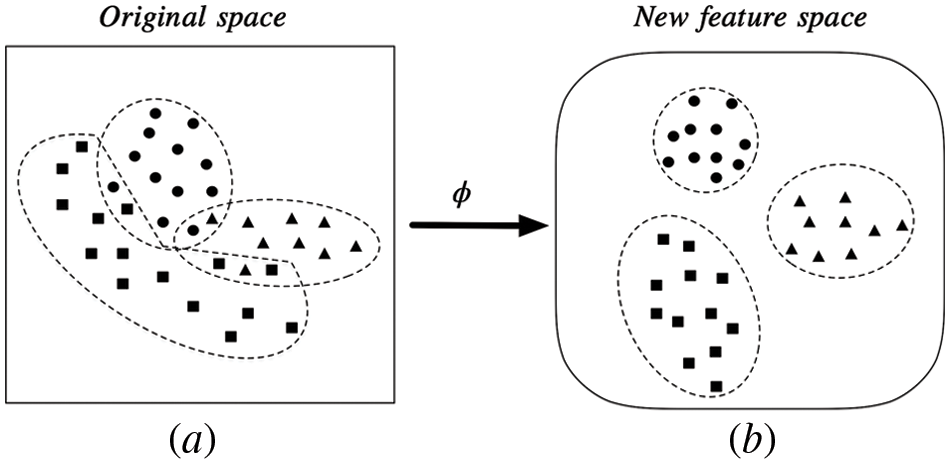
Figure 1: Metric learning. Mapping data from the original space to a new, more discriminatory special space

Deep neural networks are often used to construct mappings for metric learning due to their powerful non-linear fitting capacity. The Prototypical Network is a metric learning method that uses neural networks to learn the feature mapping of data with few labels [20]. Prototypical Network can reconfigure the spatial metric and facilitate the classification and clustering of data, therefore it and its variants are widely used in many research fields [21–23]. The Prototypical Networks divide the labeled data of a category into a Support set and a Query set. Each class center is the mean vector of the embedded support points belonging to its class. Finally, learning proceeds by minimizing a distance function between query points and the class center via Stochastic Gradient Descent (SGD).

To compensate for the shortcomings of unsupervised clustering algorithm that can not use any prior information and hard to find an appropriate distance metric for high-dimensional data, this paper combines the ideas of semi-supervised clustering and metric learning and proposes a semi-supervised clustering algorithm based on deep feature mapping (SSFM). SSFM uses a modified prototype network and a small number of data priors to learn a non-linear mapping that maps all data to a new metric space with higher discrimination, increasing the separability of the samples. The data is then clustered in this metric space. The main contributions of this paper are.

•   Applying the ideas of prototypical networks and metric learning to semi-supervised clustering and achieving good results.

•   Performing metric learning using neural networks and the learned feature mapping has a closed-form solution that enables feature mapping of unsupervised data as well.

•   Designing a new feature mapping method using a modified prototypical network loss function that allows samples of different categories to be better separated in the new feature space, with improved clustering results.

•   An algorithm is given for clustering semi-supervised data in a high-dimensional space where Euclidean distance is not applicable.

The remainder of the article is organized as follows. In Section 2, the related works are introduced. In Section 3, the metric-based K-means algorithm and the basic framework of the Prototypical Network algorithm are briefly illustrated. Our SSFM algorithm is presented In Section 4. Further more, Section 5 shows the experimental data, experimental methods, comparative experimental results, feature mapping performances and parameter impact analysis. Section 6 concludes the paper and outlooks future work.

2  Related Works

Semi-supervised clustering algorithms usually use pairs of constraints as supervised information, i.e., Must-Link and Cannot-Link constraints [24–26], where Must-Link constraint indicates that two or more samples belong to the same class. In contrast, Cannot-Link constraint indicates that two or more samples do not belong to the same class.

Semi-supervised DenPeak Clustering (SSDC) is a representative of the Semi-supervised clustering algorithms. It generates some clusters (much more than the actual number of categories) using Density Peak Clustering (DenPeak) [27] without violating the Cannot-Link constraint and then traversing all clusters. The algorithm will contact two clusters if they have sample points that satisfy the Must-Link constraint [28]. SC-Kmeans algorithm [29] is proposed for how to make full use of the efficient prior knowledge in semi-supervised clustering algorithms. The algorithm expands the pairwise constraints by using both pairwise constraints and independent class labels to obtain a new set of ML and CL constraints, which improves the clustering accuracy of K-means method. However, the efficiency of SC-algorithm is not high for processing large scale data. Semi-supervised fuzzy clustering with fuzzy pairwise constraints (SSFPC) [30] extends the traditional pairwise constraint (i.e., Must-Link or Cannot-Link) to fuzzy pairwise constraint and avoids eliminating the fuzzy characteristics. Chen et al. proposed a semi-supervised clustering algorithm (ASGL) using only pairwise relationships, learning both similarity matrices in feature space and label space, exploring the local and global structures of the data respectively, and obtaining better clustering results [31]. Yan et al. proposed the semi-supervised density peaks clustering algorithm (SSDPC) [32]. Instead of clustering in the original feature space of the data, SSDPC uses the semi-supervised information of pairwise constraints Must-Link and Cannot-Link to learn a linear mapping, where the samples of Must-Link are close to each other, and the samples of Cannot-Link are far from each other in the mapped space. Clustering is done using the classical DenPeak algorithm in the new feature space. SSDPC makes effective use of the prior information of the data and improves the clustering performance, but it still has some limitations. First, the linear mapping method used by SSDPC has difficulty handling data with more complex distributions, such as manifold data. Second, its distance metric is the Euclidean distance, which is not applicable to high-dimensional data. Third, SSDPC uses the eigendecomposition of the matrix to calculate the projection direction, which is inefficient when the amount of data is large.

The above semi-supervised clustering algorithms achieve good clustering results on low-dimensional datasets, but they cannot handle high-dimensional data because the ordinary metrics are not applicable in the high-dimensional space. Snell et al. proposed Prototypical Networks which use a small amount of supervised information and neural network embedders to map high-dimensional data to low-dimensional space, and successfully bring similar samples close to each other in low-dimensional space. But dissimilar samples are not significantly far away from each other due to its loss function. We improve the architecture of the prototype network and its loss function and propose the SSFM algorithm, which has a better feature mapping effect.

3  Preliminaries and Motivation

3.1 K-means Algorithm and Metric Learning

Many machine learning algorithms rely on metrics. For example, the K-means algorithm relies on a specific metric to assign a sample to the cluster center nearest to it. Suppose there is a dataset D={X1,X2,…,Xn}, where the number of samples is n, and the dimension of the data is m. The K-means algorithm aims to group n samples into a specified k cluster based on similarity. Each point can only be crowded into the nearest cluster center. The algorithmic procedure of K-means is summarized as follows.

Firstly, initializing k cluster centers {C1,C2,…,Ck}, 1<k≤n, and computing the distance d(Xi,Cj) between samples and each cluster center. If the distance metric is chosen as a Euclidean distance, then

d(Xi,Cj)=∑t=1m(Xit−Cjt)2(1)

where Xi denotes the ith point, 1≤i≤n; Cj denotes the jth cluster center, 1≤j≤k; Xit denotes the tth feature of the ith sample, 1≤t≤m; Cjt denotes the tth center attribute of the jth cluster. The distance of object to each cluster center is compared in turn, and the object is assigned to the cluster of the nearest cluster center to obtain k clusters {P1,P2,…,Pk}. Recalculate the cluster centers based on the obtained k clusters

Cl=1|Pl|∑Xi∈PlXi(2)

where Cl denotes the center of the lth cluster, 1≤l≤k, |Pl| denotes the number of objects in the lth cluster, Xi denotes the ith object in the lth cluster, 1≤i≤|Pl|. The distance from objects to the center of each cluster is then calculated based on the new cluster centers, and so on, iterating until the cluster centers almost not change.

However, the Euclidean distance is not applicable in all data scenarios. Choosing a good metric can improve the generalization of a model. We want to start with the data itself and find an appropriate metric for that data. Metric learning uses supervised information to map the data into a more discriminative metric space [33], which is beneficial for bringing similar samples close to each other and separating dissimilar samples under the new metric. Combining the K-means algorithm with metric learning can effectively improve the algorithm’s performance.

3.2 Prototypical Network

Similar to the semi-supervised clustering scenario, the Prototypical Network also uses a small amount of prior information to learn the essential features of the data. Snell et al. proposed the Prototypical Network structure in 2017 for solving image recognition problems in the few shot dilemmas. Denote the few shot training set as X={(x1,y1),(x2,y2),…,(xN,yN)}, which contains C classes of data with only a small number of samples in each class. The samples of each class in the training set are divided into a Support set (S) and a Query set (Q). The main idea of the prototype network is to map the data into a new feature space through metric learning. A feature prototype is found for each class on the new feature space. When the feature mapping of the image to be tested is obtained, a distance metric is applied to the mapped test image and the feature prototype of each class separately to obtain the prediction result. The class prototypes are defined as follows

ck=1|Sk|∑(xi,yi)∈Skfϕ(xi)(3)

where Sk denotes the support set for the kth class, consisting of some samples from that class. |Sk| denotes the cardinality of the set Sk, and fϕ represents the non-linear mapping, represented as a four-layer fully convolutional neural network in Snell’s article. The similarity between query points and class prototypes is represented by the SoftMax value of the negative Euclidean distance

pϕ(y=k|x)=exp⁡(−d(fϕ(x),ck))∑k′exp⁡(−d(fϕ(x),ck′))(4)

Learning proceeds by minimizing the negative log-probability J(ϕ)=−log⁡pϕ(y=k|x) of the entire Query set via gradient descent. Fig. 2 shows a schematic representation of the loss calculation of Prototypical Network in the new feature space.

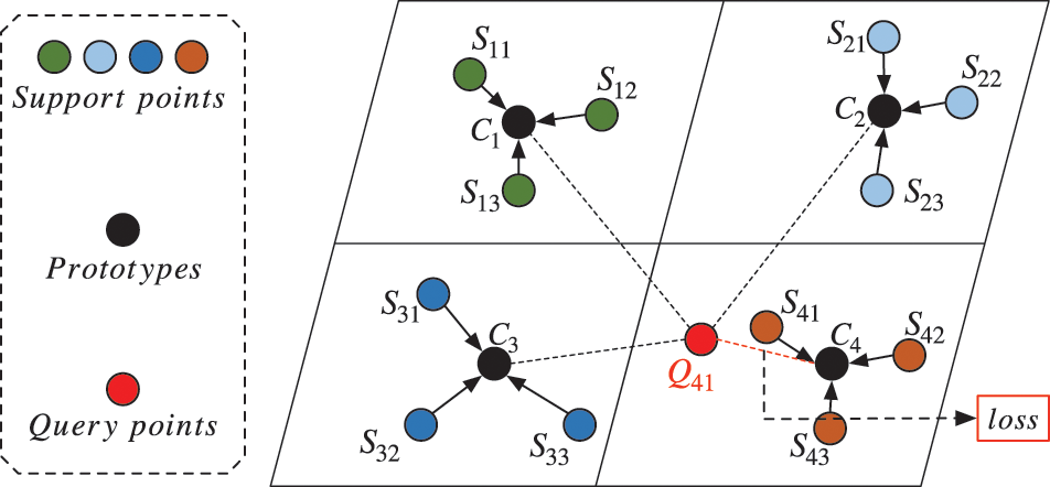
Figure 2: Prototypical Network feature space

3.3 Motivation

The semi-supervised data prior information Must-Link and Cannot-Link provide some useful prior knowledge of the data, i.e., which samples are supposed to be similar and which samples are highly divergent. With the idea and framework of the Prototypical Network, we use the prior information to learn an embedding mapping that embeds the data into a new metric space and then clusters them. Although the Prototypical Network performs well in few shot image recognition problems, applied to semi-supervised clustering it has the following shortcomings.

•   The loss function of the Prototypical Network is mainly considered to bring similar sample points closer, while the constraint on dissimilar sample points is not obvious enough, resulting in dissimilar samples not being clearly distinguished (subsequent experiments will demonstrate the existence of this problem).

•   The traditional Prototypical Network is targeted at image data and therefore constructs embedding mappings using convolutional neural networks, which cannot be extended to embedding mappings of general data.

In this paper, we propose a semi-supervised clustering algorithm based on the Prototypical Network with corrected loss, which makes the differences between the embedding of heterogeneous samples more obvious. In particular, we build the network architecture according to the type of dataset so that data of different types can be mapped to the new metric space.

4  SSFM Algorithm

The semi-supervised clustering problem is defined as to cluster the entire dataset where a large number of samples are unlabeled, with the help of a small portion of labeled samples. These labeled samples are usually called semi-supervised information. Generally, except for labels on samples, the semi-supervised information could also be given in the form of pairwise constraints or other prior information. In this paper, we mainly focus on the clustering method with pairwise constraints as semi supervised information, where a pairwise constraint has the form (Si,Sj) and Si or Sj can be a sample or a collection of samples. All the pairwise constraints are divided into two categories called Must-Link, which specifies that the samples belong to the same class, and Cannot-Link, which specifies that the samples do not belong to the same class. Suppose there are T supervised samples from each class (T typically occupies only 10\% to 20\% of all samples in each class). Supervised samples of each class constitute a Must-Link set, and supervised samples of every two class constitute a Cannot-Link sets pair. The SSFM algorithm contains three stages.

•   Firstly, learning an encoder with supervised information, i.e., Must-Link sets and Cannot-Link sets. The loss function is designed to maximize the distance between two Cannot-Link sets and minimize the distance in a Must-Link set.

•   Secondly, feature mapping all the data with the trained encoder to the new feature space.

•   Thirdly, Clustering samples in the new feature space using an unsupervised clustering algorithm.

The overall framework of the algorithm is shown in Fig. 3.

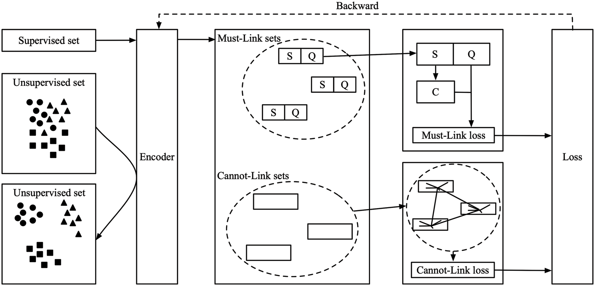
Figure 3: Overall framework of SSFM algorithm

4.1 Calculate Must-Link Loss

Denote the set of Must-Link sets as ML={M1,M2,…,Mn}, where Mk={uk,1,uk,2,…,uk,σk} indicates a Must-Link set. The samples in the Mk belong to the same class. σk is the number of samples in this set. The set of Cannot-Link sets is denoted as CL={C1,C2,…,Cm}, where Ck={ck,1,ck,2,…,ck,τk} indicates a Cannot-Link set. Any two sets in CL do not belong to the same class. τk is the number of samples in this set. Let X={x1,x2,…,xn} be a set of samples, and the center of this set is defined as

Ave(X)=1n∑i=1nxi(5)

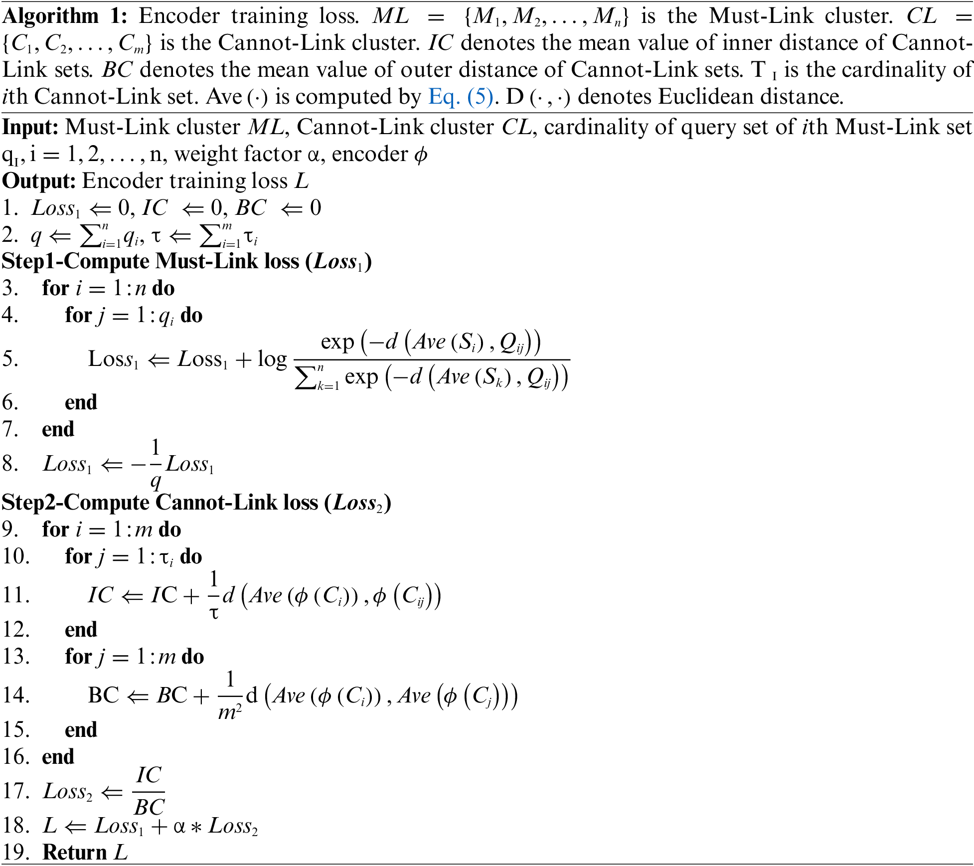
In order to keep the distance between samples in the same Must-Link set as small in the new feature space, a Must-Link set is divided into a Support set and a Query set. Let the Support set be encoded to obtain the centers of the Support set in the new feature space, and encode the Query set to obtain its feature mapping. In the new feature space, optimize the following loss function to make each point in the Query set close to the center of its Support set.

Loss1=−1∑i=1nqi∑i=1n∑j=1qilog⁡exp⁡(−d(Ave(Si),Qij))∑k=1nexp⁡(−d(Ave(Sk),Qij))(6)

where Si,Qi,i=1,2,…,n are the encoded Support set and Query set of the ith Must-Link set. Qij denotes the jth sample of the ith Query set. qi is the cardinality of the ith Query set, and d(⋅,⋅) denotes the Euclidean distance. Optimising Loss1 can simultaneously adjust the embedding of samples in S and Q so that samples of the same class are embedded in a cluster.

4.2 Calculate Cannot-Link Loss

For the data from different classes to be separated further away in the new feature space, the intraclass distance of any two Cannot-Link sets should be as large as possible compared to the interclass distance. Cannot-Link loss function is designed as

Loss2=1∑i=1mτi∑i=1m∑j=1τid(Ave(ϕ(Ci)),ϕ(Cij))1m2∑i,j=1md(Ave(ϕ(Ci)),Ave(ϕ(Cj)))(7)

where ϕ indicates the feature mapping function. Cij denotes the jth sample of the ith Cannot-Link set, and τi denotes the cardinality of the ith Cannot-Link set.

The final loss function of the algorithm L is defined as

L=Loss1+α ∗ Loss2(8)

where α is a weighting factor to balance the contribution of the two components. Optimize the loss via gradient descent and adjust the parameters in the encoder until the loss falls steady. This process is described in Algorithm 1.

4.3 Encoder Designs

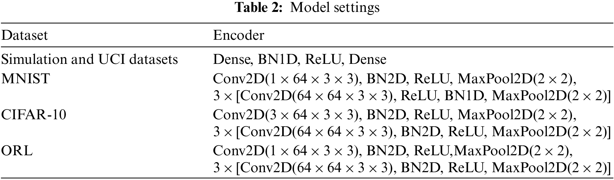
Different encoders apply to diverse semi-supervised clustering data. For low-dimensional data, a fully connected neural network is adequate. However, a multi-layer convolutional neural network is more suitable for high-dimensional data, such as image data. Convolutional neural networks have the advantage of local connectivity and shared parameters, reducing the trained parameters. Furthermore, convolutional neural networks can use the original image as input, avoiding a complex feature extraction process. CNN perceives the local pixels of the image, which can effectively learn the corresponding features from many samples [34]. The data is input into the trained encoder and crowded into various clusters in the new feature space via an unsupervised clustering algorithm e.g., K-means.

5  Experimental Analysis

5.1 Experimental Datasets

We conducted experiments on the simulation datasets, the University of California Irvine (UCI) datasets, and the image datasets, respectively. The simulation datasets include Aggregation (Aggr) and Jain. The UCI real-world datasets include Iris, Wine, Synthetic Control, Glass Identification, Balance Scale and Letter-Recognition (only data of the letter D, O and Q). In addition, we also run experiments on three image datasets, including the MNIST dataset (selecting 1,000 samples from each class), the CIFAR-10 dataset (selecting 500 samples from each class), and the ORL face image dataset (selecting 10 samples from each people). Table 1 shows the specific number of samples, feature dimensions, and categories for each dataset.

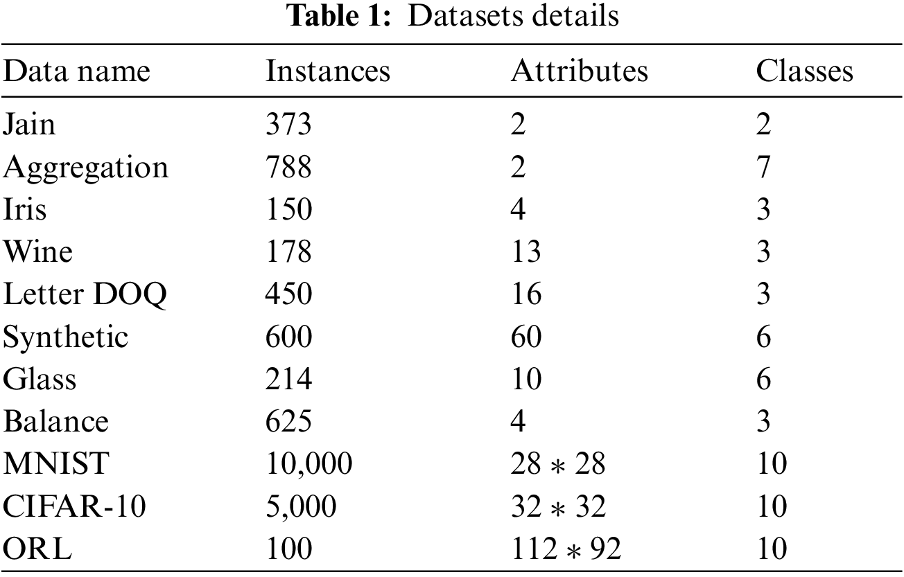
The UCI real-world datasets can be found at https://archive.ics.uci.edu/ml/datasets.php.

The MNIST dataset can be found at http://yann.lecun.com/exdb/mnist/.

The CIFAR-10 dataset can be found at https://www.cs.toronto.edu/~kriz/cifar.html.

The ORL dataset can be found at http://www.cl.cam.ac.uk/research/dtg/attarchive/facedatabase.html.

5.2 Model Evaluation Indicators

Various metrics have been proposed for the evaluation of clustering algorithms, such as the Adjusted Mutual Information (AMI) [35] and the Adjusted Rand Index (ARI) [36]. The AMI and the ARI have [−1,1] value range. The higher values indicate a better clustering result. In addition, we used the 1-nearest neighbor (1NN) classification accuracy to evaluate the performance of feature mapping. A high 1NN classification accuracy means that the original data are easier to distinguish after feature mapping. We compared our algorithm with some classical unsupervised clustering and semi-supervised clustering algorithms, including K-means, DBSCAN, DenPeak, SSDC, SSDPC, SC-Kmeans and Proto-Net.

5.3 Experimental Method

The supervised information is obtained by randomly selecting a small fraction (typically 20%) of data from each class to form the Must-Link sets and the Cannot-Link sets. To ensure the amount of supervised information is identical in different algorithms, we converted all the samples in the Must-Link sets and the Cannot-Link sets into pairs constraints, which have the same number as other semi-supervised clustering algorithms.

The encoder was designed as a fully connected neural network with only one hidden layer for the low-dimensional datasets, including Aggregation, Jain, Iris, Wine, Letter DOQ, Synthetic, Balance, and Glass. In addition, we designed the encoder as a four-layer fully convolutional neural network for the image datasets. The convolutional kernel size was 3×3 and the max-pooling kernel size was 2×2. We use Rectified Linear Unit (ReLU) as an activation function, Batch Normalization (BN) as regularization method and use the Adam algorithm to optimize the loss. The model settings are presented in Table 2.

5.4 Experimental Results

Each algorithm was performed 10 times for each dataset. The average ARI and AMI are shown in Tables 3 and 4 The best results on each dataset are bolded.

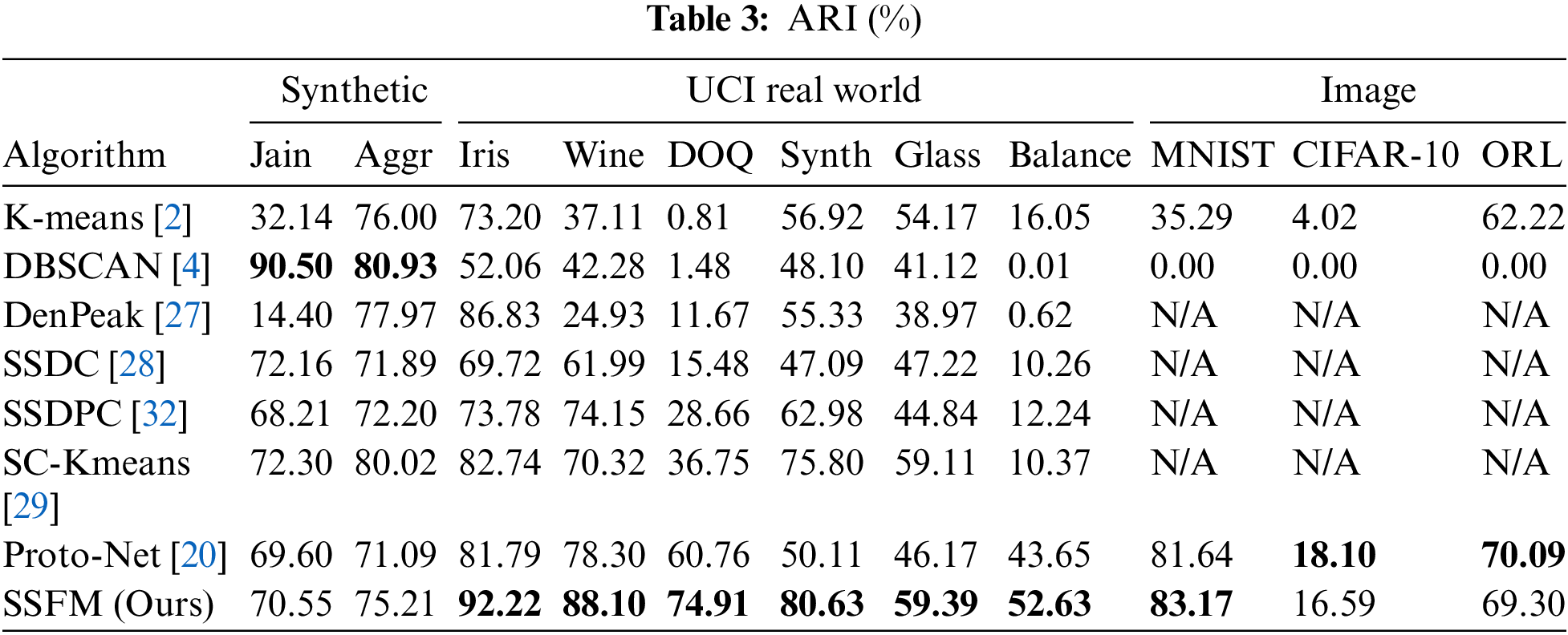
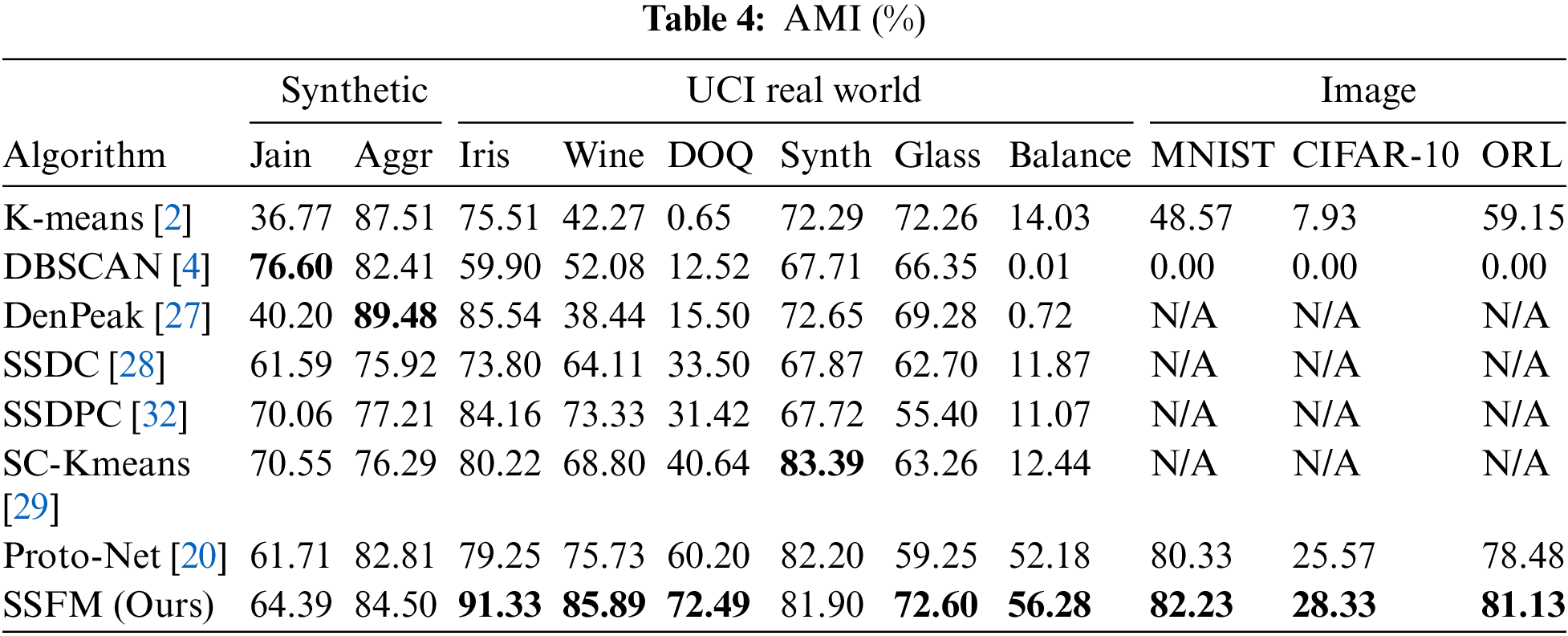
Tables 2 and 3 show that SSFM outperforms other clustering algorithms for high-dimensional data and also perform well in low-dimensional data, especially on the DOQ dataset. For the five low-dimensional datasets of Iris, Wine, DOQ, Synthetic and Glass Balance, the clustering performance of SSFM is significantly better than the other seven clustering algorithms. For the Jain and Aggregation datasets, density-based clustering algorithms such as DBSCAN and DenPeak achieved better clustering results because these two datasets are non-convex datasets. Density-based clustering algorithms have better clustering results for such irregularly structured datasets. SSFM also has better clustering results on two high-dimensional image datasets, MNIST and ORL, due to the fact that the metric loss designed in SSFM optimizes the parameters of the convolutional neural network constructed for the image data, extracting features of the images that are conducive to clustering. However, the SSFM and the Proto-Net algorithms do not perform well for the CIFAR-10 dataset. The reason may be that the encoder only uses the simplest four-layer fully convolutional neural network, which cannot extract many valuable features for three-channel images.

5.5 Feature Mapping Results

Let γ=0.2 and α=0.5. The SSFM algorithm map the four datasets, including Iris, Wine, Letter DOQ, and Synthetic, into the three-dimensional feature space. Fig. 4 demonstrates the performance of feature mapping. It shows that the SSFM algorithm effectively maps similar samples to one cluster and heterogeneous samples separate from each other in the new feature space, which is more beneficial for unsupervised clustering algorithms to group data. In addition, Figs. 5 and 6 show the results of the image dataset ORL and MNIST projected to a two-dimensional feature space by the SSFM algorithm. SSFM successfully mapped the photos of different persons’ faces to different clusters in the feature space. The clusters of person1, person3 and person9 have a little overlap occurring, while the clusters of the remaining seven people can be clearly separated. The images of each category of the MNIST dataset are also mapped into distinct clusters that are clearly differentiated.

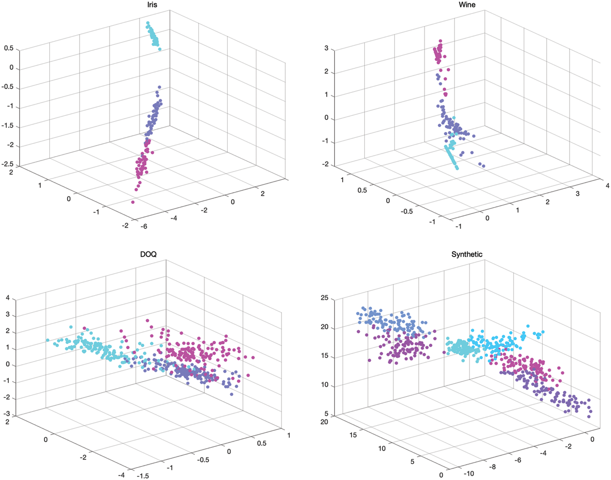
Figure 4: Mapping of Iris, Wine, Letter DOQ, Synthetic datasets in the 3D feature space

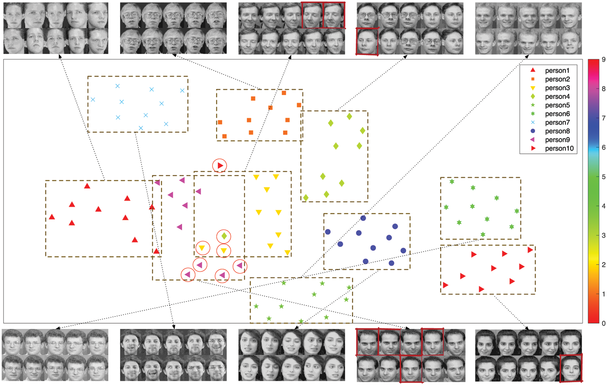
Figure 5: 2D features of the ORL face dataset by SSFM feature mapping. The outliers have been circled in red and the corresponding face images have been marked with red boxes

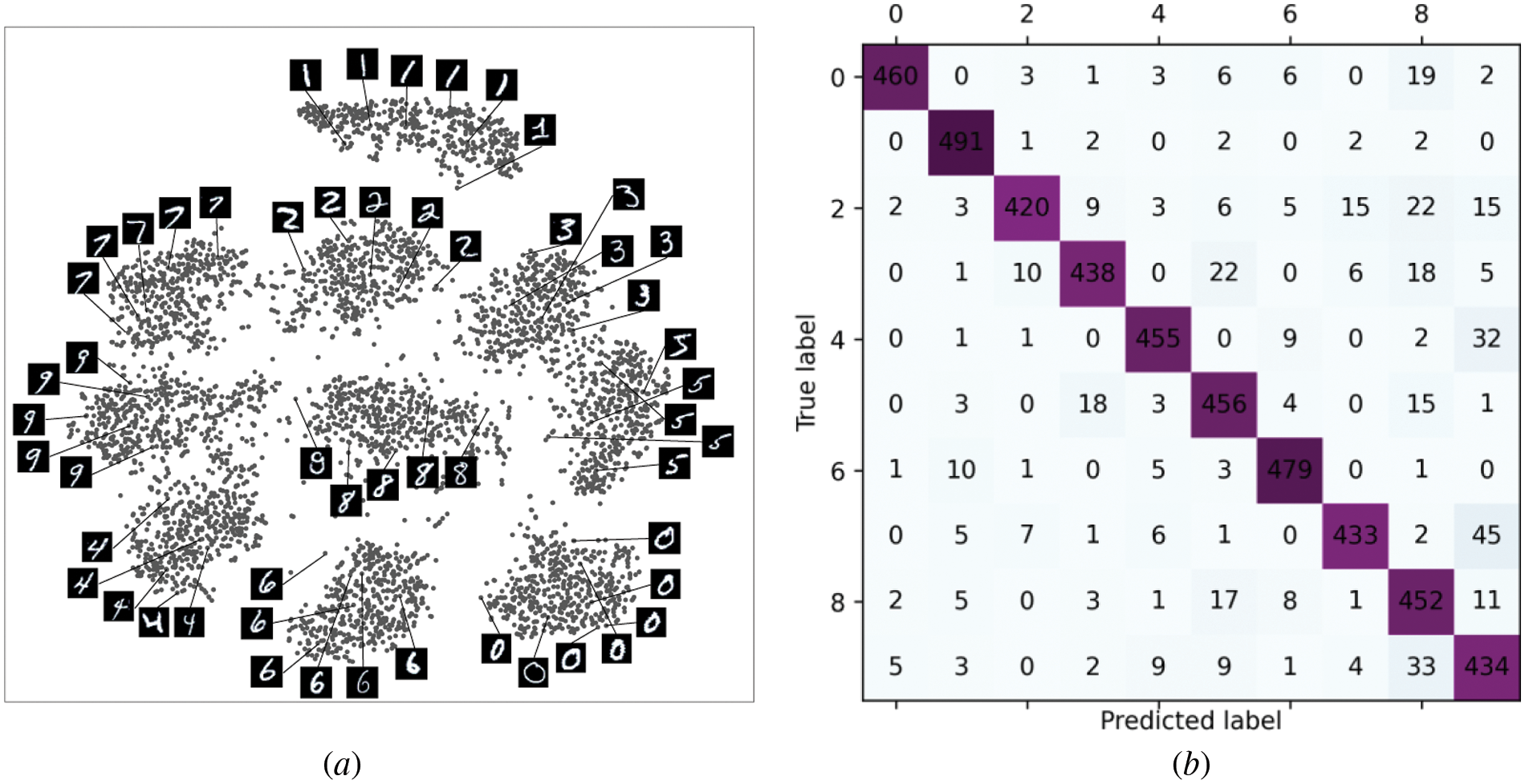
Figure 6: (a) 2D features of the MNIST dataset after SSFM feature mapping. (b) Confusion matrix of labels predicted by clustering in new feature space and true labels

In addition, we demonstrate the data feature mapping performance of SSFM algorithm, Proto-Net algorithm and PCA on two datasets, including Wine and DOQ. Fig. 7 shows the mapping results. The performance of PCA was poor because it did not use the supervised information at all. SSFM and Proto-Net both mapped different classes of data into different clusters. However, SSFM can separate the data of different classes further than Proto-Net and be more able to reflect the differences between the data in the new feature space. The reason for this is that the loss of SSFM considers separating the Cannot-Link of the sample sets in the embedding feature space from each other, whereas Proto-Net does not consider it.

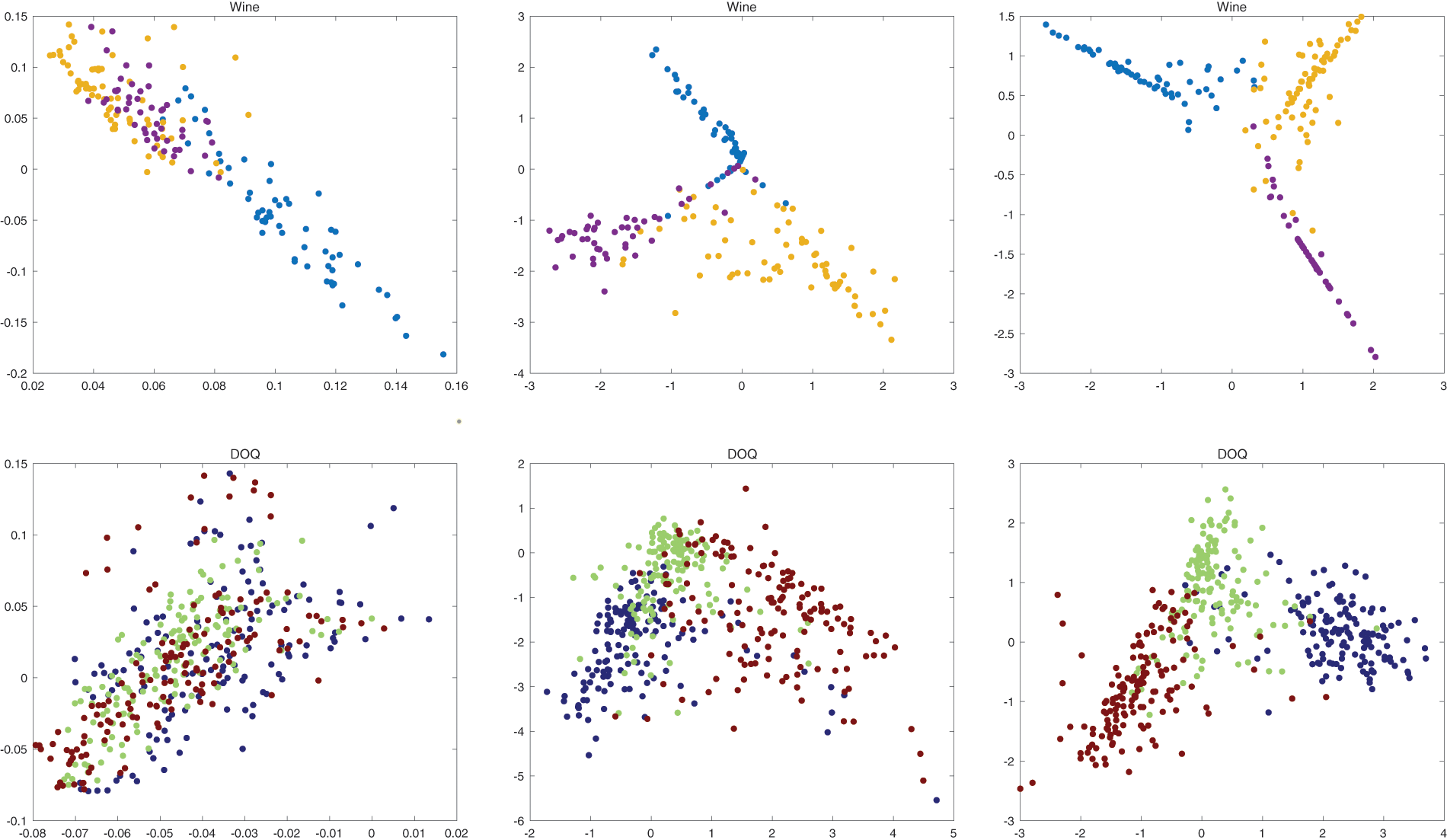
Figure 7: Wine, Letter DOQ datasets mapped by PCA (left), Proto-Net (middle) and SSFM (right) for 2D features

5.6 Parameter Impact Analysis

Two parameters, including the loss function weight factor α and the ratio of supervised information to the total data γ, influence the performance of feature mapping. We analyze their effect on different datasets. Firstly, fix the proportion of supervised information γ=0.2 and adjust the value of the weighting factor α. Secondly, fix the value of the weighting factor α=0.5 and adjust the proportion of supervised information γ. The classification accuracy of the 1NN classifier was chosen as the metric of feature mapping effectiveness. Specifically, the whole data embedded into the new feature space was divided into a training set and a test set on a 7:3 ratio. The 1NN classifier was trained to classify the test set. Fig. 8 shows the impact of the parameters on Iris, Wine, Letter DOQ, and Synthetic datasets.

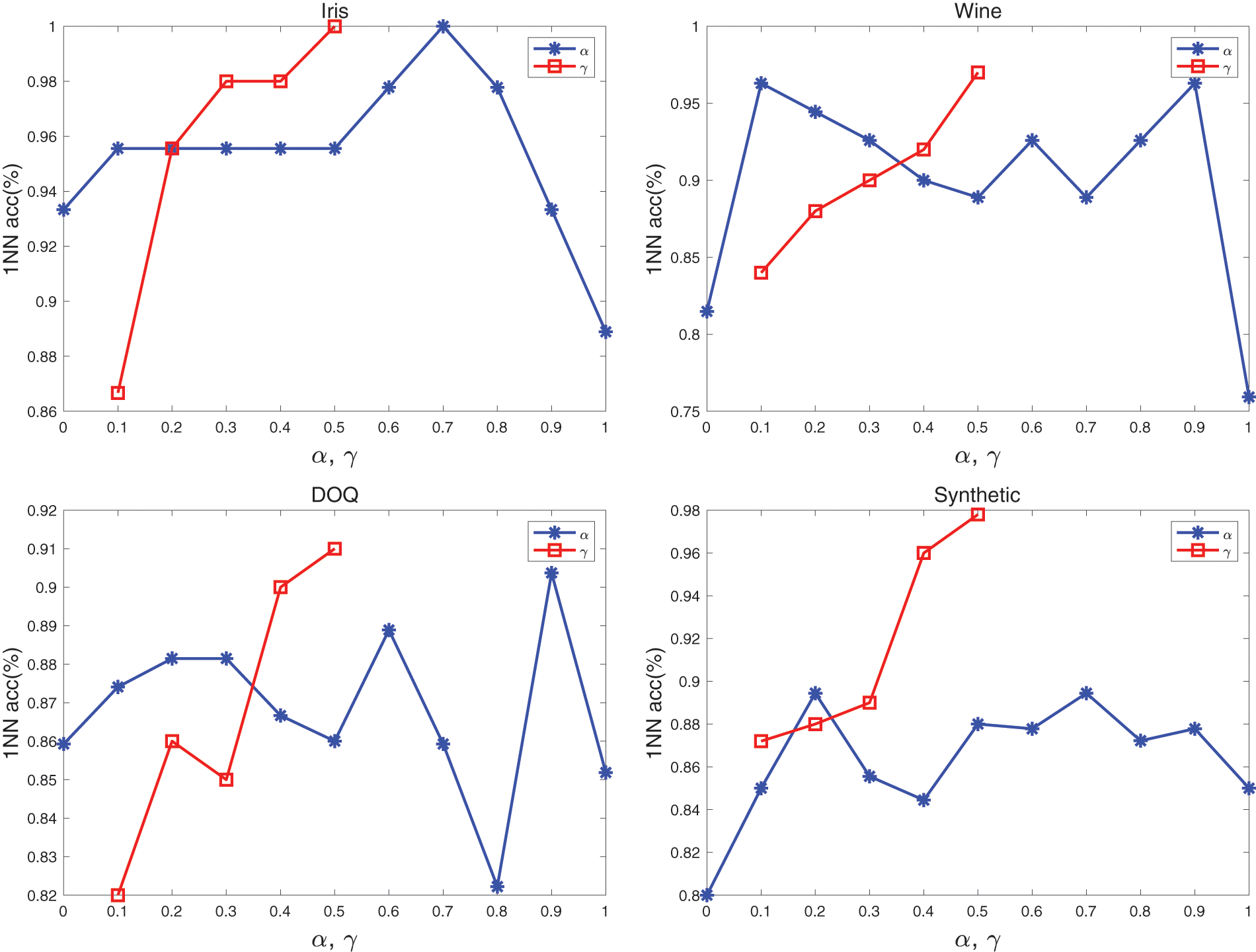
Figure 8: The effect of loss weighting factor α and supervisory information proportion γ

α=0 means not considering maximizing the distance between the Cannot-Link sets. The results show that the Cannot-Link loss is effective. Moreover, even using a small amount of supervised information, the feature mapping performance is still better than that of the model using more supervised information by choosing an appropriate α. More supervised information will result in better feature mapping if the loss function is consistent.

6  Conclusion

This paper presents a semi-supervised clustering algorithm (SSFM) based on metric learning and prototype networks. By designing an appropriate network structure and loss function, the algorithm can learn a feature mapping using semi-supervised information (Must-Link, Cannot-Link). This mapping embeds the original data into a new metric space and allows samples of the same type to be placed close to each other and samples of different types to be separated, thus making the data easier to cluster. Experiments were conducted on synthetic and real-world data (including low and high dimensional data), and the mapped data were passed to 1NN classification and K-means clustering. The experimental results show that the mapped data have significantly better classification and clustering results compared with the original data. Furthermore, by comparing classical unsupervised and semi-supervised clustering algorithms on a variety of datasets using common clustering metrics (ARI, AMI), the experimental results validate the effectiveness and robustness of the SSFM algorithm. SSFM algorithm requires a small amount of supervised information for each class of data, otherwise it will lead to undesirable clustering results, which is a limitation of the algorithm. One solution is to first label the data with a small number of pseudo-labels by an unsupervised clustering algorithm. Re-utilizing the semi-supervised information of the data in the new feature space to assist clustering is a future work to be accomplished.

Funding Statement: The authors received no specific funding for this study.

Conflicts of Interest: The authors declare that they have no conflicts of interest to report regarding the present study.

References

1. R. Xu and D. Wunsch, “Survey of clustering algorithms,” IEEE Transactions on Neural Networks, Materials & Continua, vol. 16, no. 3, pp. 645–678, 2005. [Google Scholar]

2. J. MacQueen, “Some methods for classification and analysis of multivariate observations,” in Proc. of the Fifth Berkeley Symp. on Mathematical Statistics and Probability, Oakland, CA, USA, vol. 1, 1967. [Google Scholar]

3. D. Comaniciu and P. Meer, “Mean shift: A robust approach toward feature space analysis,” IEEE Transactions on Pattern Analysis and Machine Intelligence, vol. 24, no. 5, pp. 603–619, 2002. [Google Scholar]

4. M. Ester, H. P. Kriegel, J. Sander and X. xu, “A Density-based algorithm for discovering clusters in large spatial databases with noise,” in Proc. of the Second Int. Conf. on Knowledge Discovery and Data Mining, Portland, Oregon, pp. 226–231, 1996. [Google Scholar]

5. Y. Xie, S. Shekhar and Y. Li, “Statistically-robust clustering techniques for mapping spatial hotspots: A survey,” ACM Comput. Surv., vol. 55, no. 2, pp. 1–38, 2022. [Google Scholar]

6. W. Ma, X. Tu, B. Luo and G. Wang, “Semantic clustering based deduction learning for image recognition and classification,” Pattern Recognit., vol. 124, pp. 108440, 2022. [Google Scholar]

7. A. Nazir, M. N. Cheema, B., Sheng, P. Li, H. Li et al., “ECSU-Net: An embedded clustering sliced U-net coupled with fusing strategy for efficient intervertebral disc segmentation and classification,” IEEE Trans. Image Process., vol. 31, pp. 880–893, 2022. [Google Scholar] [PubMed]

8. G. Gilam, E. M. Gramer, K. A. Webber, M. S. Ziadni, M. C. Kao et al., “Classifying chronic pain using multidimensional pain-agnostic symptom assessments and clustering analysis,” Science Advances, vol. 7, no. 37, pp. eabj0320, 2021. [Google Scholar] [PubMed]

9. Y. Xie, D. Feng, X. Shen, Y. Liu, J. Zhu et al., “Clustering feature constraint multiscale attention network for shadow extraction from remote sensing images,” IEEE Trans. Geosci. Remote. Sens., vol. 60, pp. 1–14, 2022. [Google Scholar]

10. C. Mao, H. Liang, Z. Yu, Y. Huang and J. Guo, “A clustering method of case-involved news by combining topic network and multi-head attention mechanism,” Sensors, vol. 21, no. 22, pp. 7501, 2021. [Google Scholar] [PubMed]

11. Y. Cheng, M. Cheng, T. Pang and S. Liu, “Using clustering analysis and association rule technology in cross-marketing,” Complex., vol. 2021, pp. 9979874:1–9979874:11, 2021. [Google Scholar]

12. B. S. Everitt, S. Landau and M. Leese, “Cluster analysis arnold,” A Member of the Hodder Headline Group, London, pp. 429–438, 2001. [Google Scholar]

13. Y. Yu, G. Yu, X. Chen and Y. Ren, “Semi-supervised multi-label linear discriminant analysis,” in Neural Information Processing, Cham, Springer International Publishing, pp. 688–698, 2017. [Google Scholar]

14. Z. Yu, P. Luo, J. You, H. S. Wong, H. Leung et al., “Incremental semi-supervised clustering ensemble for high dimensional data clustering,” IEEE Transactions on Knowledge and Data Engineering, vol. 28, no. 3, pp. 701–714, 2016. [Google Scholar]

15. J. B. Tenenbaum, V. de Silva and J. C. Langford, “A global geometric framework for non-linear dimensionality reduction,” Science, vol. 290, no. 5500, pp. 2319–2323, 2000. [Google Scholar] [PubMed]

16. S. T. Roweis and L. K. Saul, “Non-linear dimensionality reduction by locally linear embedding,” Science, vol. 290, no. 5500, pp. 2323–2326, 2000. [Google Scholar] [PubMed]

17. Y. Feng, Y. Yuan and X. Liu, “Person reidentification via unsupervised cross-view metric learning,” IEEE Transactions on Cybernetics, vol. 51, no. 4, pp. 1849–1859, 2021. [Google Scholar] [PubMed]

18. Y. Yuan, J. Lu, J. Feng and J. Zhou, “Deep localized metric learning,” IEEE Transactions on Circuits and Systems for Video Technology, vol. 28, no. 10, pp. 2644–2656, 2018. [Google Scholar]

19. G. J. Liu, H. Chen, L. Y. Wang and D. Zhu, “Metric learning based similarity measure for attribute description identification of energy data,” in 2020 Int. Conf. on Machine Learning and Cybernetics, Online, pp. 219–223, 2020. [Google Scholar]

20. J. Snell, K. Swersky and R. Zemel, “Prototypical networks for few-shot learning,” in Advances in Neural Information Processing Systems, Long Beach, pp. 4077–4087, 2017. [Google Scholar]

21. Y. Li, Z. Ma, L. Gao, Y. Wu, F. Xie et al., “Enhance prototypical networks with hybrid attention and confusing loss function for few-shot relation classification,” Neurocomputing, vol. 493, pp. 362–372, 2022. [Google Scholar]

22. H. Tang, Z. Huang, Y. Li, L. Zhang and W. Xie, “A multiscale spatial–Spectral prototypical network for hyperspectral image few-shot classification,” IEEE Geoscience and Remote Sensing Letters, vol. 19, pp. 1–5, 2022. [Google Scholar]

23. W. Fu, L. Zhou and J. Chen, “Bidirectional matching prototypical network for few-shot image classification,” IEEE Signal Processing Letters, vol. 29, pp. 982–986, 2022. [Google Scholar]

24. S. Xiong, J. Azimi and X. Z. Fern, “Active learning of constraints for semi-supervised clustering,” IEEE Transactions on Knowledge and Data Engineering, vol. 26, no. 1, pp. 43–54, 2014. [Google Scholar]

25. N. M. Arzeno and H. Vikalo, “Semi-supervised affinity propagation with soft instance-level constraints,” IEEE Transactions on Pattern Analysis and Machine Intelligence, vol. 37, no. 5, pp. 1041–1052, 2015. [Google Scholar] [PubMed]

26. H. Zeng and Y. Cheung, “Semi-supervised maximum margin clustering with pairwise constraints,” IEEE Transactions on Knowledge and Data Engineering, vol. 24, no. 5, pp. 926–939, 2012. [Google Scholar]

27. A. Rodriguez and A. Liao, “Clustering by fast search and find of density peaks,” Science, vol. 344, no. 6191, pp. 1492–1496, 2014. [Google Scholar]

28. Y. Ren, X. Hu, K. Shi, G. Yu, D. Yao et al., “Semi-supervised DenPeak clustering with pairwise constraints,” in PRICAI 2018: Trends in Artificial Intelligence, Cham, Springer International Publishing, pp. 837–850, 2018. [Google Scholar]

29. Z. Chen, H. Wang and M. Hu, “An active semi-supervised clustering algorithm based on seeds set and pairwise constraints,” J. Jilin Univ.(Sci. Ed.), vol. 55, no. 3, pp. 664–672, 2017. [Google Scholar]

30. Z. Wang, S. Wang, L. Bai, W. Wang and Y. Shao, “Semisupervised fuzzy clustering with fuzzy pairwise constraints,” IEEE Transactions on Fuzzy Systems, vol. 30, no. 9, pp. 3797–3811, 2022. [Google Scholar]

31. L. Chen and Z. Zhong, “Adaptive and structured graph learning for semi-supervised clustering,” Information Processing & Management, vol. 59, no. 4, pp. 102949, 2022. [Google Scholar]

32. S. Yan, H. Wang, T. Li, J. Chu and J. Guo, “Semi-supervised density peaks clustering based on constraint projection,” International Journal of Computational Intelligence Systems, vol. 14, no. 1, pp. 140–147, 2021. [Google Scholar]

33. Y. Li, X. Fan and E. Gaussier, “Supervised categorical metric learning with schatten p-norms,” IEEE Transactions on Cybernetics, vol. 52, no. 4, pp. 2059–2069, 2022. [Google Scholar] [PubMed]

34. Y. Lecun, L. Bottou, Y. Bengio and P. Haffner, “Gradient-based learning applied to document recognition,” Proceedings of the IEEE, vol. 86, no. 11, pp. 2278–2324, 1998. [Google Scholar]

35. A. Amelio and C. Pizzuti, “Correction for closeness: Adjusting normalized mutual information measure for clustering comparison,” Computational Intelligence, vol. 33, no.3, pp. 579–601, 2017. [Google Scholar]

36. N. X. Vinh, J. Epps and J. Bailey, “Information theoretic measures for clusterings comparison: Is a correction for chance necessary?,” in Proc. of the 26th Annual Int. Conf. on Machine Learning, New York, NY, USA, pp. 1073–1080, 2009. [Google Scholar]