Learning-Related Sentiment Detection, Classification, and Application for a Quality Education Using Artificial Intelligence Techniques

1  Introduction

The evolution of technologies has made the reach of the internet to the masses. This revolution in communication via the internet has demolished the geographical boundaries among the people. People are adopting social media to voice their sentiments and thus great amount of sentiments can be observed over the internet. Understanding sentiment of people is important for the stakeholders. Although this machine learning technique has been quite successful in many situations and applications, at the same time it still has some limitations in many real-world problems. This limitation is due to a lack abundance of sufficient data for the training. Data collection is a tedious task as it needs a lot of time, effort, and resources. This problem of data collection can be addressed to a certain extent by using a semi-supervised approach. These sentiments collected can be used to train the algorithm to transfer learning [1].

Transfer learning, on the other hand, allows for various domains, tasks, and distributions in training and testing. The study of transfer learning is driven by the idea that humans can intelligently apply previously acquired knowledge to solve new issues faster or more effectively. Learning to learn, life-long learning, knowledge transfer, inductive transfer, multi-task learning, knowledge consolidation, context-sensitive learning, knowledge-based inductive bias, meta-learning, and incremental/cumulative learning have all been terms used to describe transfer learning research since 1995 [2]. Uncovering the common (latent) traits that can help each particular activity is one method for multi-task learning. The multi-task learning framework [3], which aims to learn many tasks simultaneously even when they are dissimilar, is a closely linked learning technique to transfer learning. The discovery of shared (latent) traits that can help each particular activity is a frequent technique for multi-task learning.

The Defense Advanced Research Projects Agency’s Information Processing Technology Office (IPTO) issued Broad Agency Announcement (BAA) 05-29 in 2005, establishing a new mission of transfer learning, the ability of a system to recognize and apply knowledge and skills learned in previous tasks to novel tasks. Transfer learning, according to this definition is “the process of extracting knowledge from one or more source tasks and applying it to a target task”. Transfer learning, unlike multi-task learning, focuses on the target task rather than learning all of the source and target tasks at the same time. The source and target tasks’ roles in transfer learning are no longer symmetric.

The use of the existing model to train the new model is referred to as transfer learning. The term transfer learning was introduced by [4] as transfer of training theory and defined as “What is learned in one sphere of activity ‘transfers’ to another sphere only when the two spares share common ‘elements’”. The proposed approach is referred to as the ‘Connectionist’ learning theory. This establishes the relation between the sense of impression and impulses to action. Transfer learning has been categorized into two phases namely the training phase and the testing phase. In the testing phase, three behaviors can be observed, and these are improvement in learning, no improvement, or deterioration in learning. The concept is well accepted in education and learning as knowledge is formally transferred to the learners. Figs. 1 and 2 show traditional machine learning and transfer learning respectively.

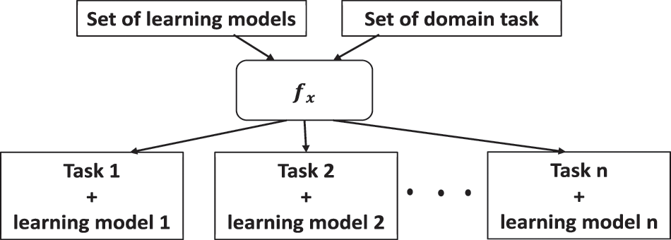
Figure 1: Traditional machine learning

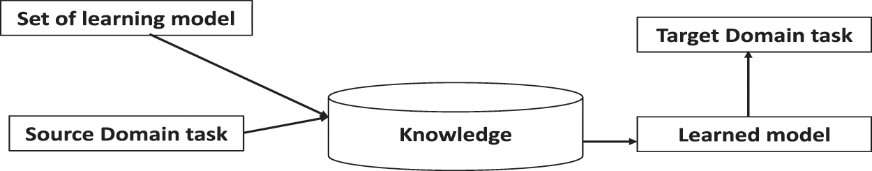
Figure 2: Transfer learning

To understand the term transfer learning, the following section briefly provides the taxonomy of transfer learning approaches.

1.1 Taxonomy of Transfer Learning Approaches

The term "transfer" refers to the effect of previous learning on the current situation. Individuals’ diverse knowledge and emotional experiences determine the rate of learning. There are three types of transfer learning listed in the literature, namely: positive learning, negative learning, and neutral learning. Transfer learning has also been classified into different categories, as discussed in the section below.

1.1.1 Homogenous Transfer Learning

Authors in [5–9] present studies covering similar exchange learning arrangements. What is more, they are isolated into subsections that relate to the exchange classifications of instance-based, highlight-based (both topsy-turvy and symmetric), boundary-based, and social-based. The technique of homogeneous exchange learning is straightforwardly pertinent to a significant information condition.

The papers [6,10] presented a method for homogenous transfer learning in their studies and showed that to bridge the gap between different domains during the data distributions, a cross-domain transfer can be considered. However, a major issue addressed in the current literature [11–13] is the domain adaptation of homogeneous learning. As a solution to this issue, executing a common or single task across various domains can result in reducing the accuracy because of the distribution shift.

1.1.2 Instance-Based Transfer Learning

In the instance-based approach, the data from the source domain cannot be used directly. However, some of these data can be then utilized to learn the targeted domain. This can be done by combining some instances from the source data domain with some of the target-labeled data and then adjusting the weight if needed. As a result, instance-based transfer learning tends to shrink the conditional/marginal distribution difference between (source/targeted domains) by utilizing some important samples or reweighting methods. Therefore, the purpose of the instance-based approach is to detect the proper weights from the labeled data in the source domain and then try to learn the source function with low expected risk when employing the targeted domain. The main goal of this method is to find the right way to figure out the expected risk based on the source distribution [14].

1.1.3 Asymmetric Feature-Based Transfer Learning

The research in [15] proposes a basic space variation calculation, alluded to as the element growth strategy (FAM). In an exchange learning condition, there are situations where an element in the source area may have an alternate significance in the outside area. The issue is alluded to as setting a highlight predisposition, which causes the contingent disseminations between the source and target areas to appear as something else.

1.1.4 Symmetric Feature-Based Transfer Learning

The work proposed in [5,16] proposes a component change approach for area variation called move segment examination (TCA), which does not require named target information. The objective is to find usual idle highlights that have the equivalent minimal appropriation over the source and target areas while keeping up the inherent structure of the first area information. The dormant highlights are found between the source and target areas in a recreating portion of Hilbert space, utilizing the most extreme mean inconsistency as a negligible circulation estimation measure. When the dormant highlights are discovered, conventional AI is used to prepare the last objective classifier. The exchange learning strategies tried are from Blitzer and Huang. The TCA technique played out the best, followed by the Huang approach and the Blitzer approach. The work by Pan proposes a ghastly element arrangement (SFA) move learning calculation that finds another component portrayal for the source and target space to determine the minor conveyance contrasts [17,18].

1.1.5 Parameter-Based Transfer Learning

Parameter-based transfer learning links the source with the targeted domain by assuming that both include related knowledge. In this approach, the model learns from the labeled source data–which is called parameters–then shares these parameters with the targeted domain [19]. Thus, the prior distributions of the parameters are shared between the source and targeted domains, which can then be transferred to the target domain prediction function to reduce the classification errors as a result. As addressed in many studies [14,17,19], the issue with performing parameter-based transfer learning is that the source and target domains should be categorized well and related, as well as the number of well-known parameters should be determined correctly in prior of training the model to achieve a significant improvement in performance. As suggested in [14], using a multi-model knowledge transfer will help to get good performance.

1.1.6 Relational Activated Transfer Learning

This approach tends to find the relationship among source data domains and then convey this relational knowledge to the targeted domain. This approach is useful when the data sample is not distributed independently and identically [14,20]. In [20], researchers propose a method for domain adaptation to solve the text classification problem when the data in the target domain is not labeled, although a huge amount of labeled data exists in the source domain. In their study, relational-based transfer learning is used to learn relational knowledge based on their precise classification into predefined classes (sentiments, topics, or neither). One of the issues of this approach [6,14,18] is to determine the suitable relational knowledge to classify the data in the target domain and achieve high performance.

By learning linguistics, furthermore, sentence structure examples of the source, a typical example is found between the source and target areas, which is utilized to foresee the subject words in the objective. The feeling words go about as an average linkage or scaffold between the source and target areas. A bipartite word chart is utilized to speak to and score the sentence structure designs. A bootstrapping calculation is used to iteratively assemble an objective classifier from the two areas. The bootstrapping procedure begins with characterization seeds, which are occurrences from the source that match the designs in the objective. A cross-space classifier is then prepared with the seed data and extricated target data (there is no objective data in the principal emphasis). The classifier is utilized to anticipate the target marks, and the top certainty evaluated target cases are chosen to remake the bipartite word diagram. The bipartite word chart is presently used to select new objective facts that are added to the seed list. This bootstrapping procedure proceeds over a chosen number of cycles, and the cross-space classifier learned in the bootstrapping process is currently accessible to anticipate target tests. This strategy is alluded to as the Social Adaptive Bootstrapping (RAP) approach.

1.1.7 Heterogeneous Transfer Learning

Independent exchange learning is where the source and target spaces are used in various component spaces. There are numerous applications where independent mobile learning is useful. This section covers a variety of exchange learning applications, including image recognition, multilanguage text order, single language text arrangement, sedate adequacy characterization, human action grouping, and programming flaw order. Independent exchange learning is likewise legitimate material for a significant information condition. As large data stores become more accessible, there is a desire to use this productive asset for AI projects, avoiding the ideal and potentially costly collection of new data. On the off chance that there is an accessible dataset drawn from a target area of intrigue that has an alternate element space from another real dataset (additionally drawn from a similar objective space), at that point, independent exchange learning can be used to connect the distinctions in the element spaces and construct a prescient model for that target space. Independent exchange learning is still a relatively new field of study, with the majority of works on the subject published in the last five years. From an elevated level view, there are two principal ways to deal with comprehending the differences, including space contrast. The awry change approach is best utilized when a similar class case in the source and target can be changed without setting a highlight inclination. Vast numbers of the different moving learning arrangements reviewed make the correct or definite suspicion that the source and the outside area occasions are drawn from a similar space.

In this approach, the feature spaces between the source domain and the targeted domain are commonly non-overlapping and non-equivalent. Thus, heterogeneous transfer learning needs to (1) handle the differences in cross-domain data distribution and (2) use feature-label space transformations to bridge the gap for knowledge transformation. As a result, this would be more challenging as there are fewer representational commonalities among the domains. In Particular, knowledge information exists in the source data. However, it is represented differently in the target data. The issue is how to implement the heterogenous transfer learning model correctly to extract the knowledge information [8,10,19].

This paper addresses the issue of learners, learning emotions. In order to capture the emotions and learning sentiments of the learners a survey was conducted among the students. Data collected was cleaned and analyzed for the further research.

The paper is organized into five sections Section 2 will discuss the methods and in Section 3 results will be discussed followed by a discussion of the results in Section 4 and the conclusion is in Section 5.

2  Materials and Methods

2.1 Experiment

In general, there are primarily two approaches (from the model training perspective) that can be used for analyzing sentiments from the text. The first approach is to create a model from scratch which includes managing and preprocessing data and lexicons. The second approach is to reuse the existing model. While the first approach consumes a lot of time, and it may be costly to develop the labelled dataset. On the contrary, the second approach can be faster but less accurate if the domain of the pre-trained model is different than the one you are targeting. However, with transfer learning, this research aims to utilize the key features of both approaches. The experiment has been designed to first extract the meaningful features from an existing pre-trained model and then the top layers of the model are retrained to learn the key features for the targeted domain from the data collected by the survey.

2.2 Dataset

We collected a dataset (https://forms.office.com/r/rAEKpmDw7X) through a targeted survey designed to understand the students’ opinions and sentiments towards learning-related sentiment detection and classification. The survey was designed to develop a sentiment database of learners’ feedback that encompasses the primary areas related to the quality of education such as lecture and content quality, learning environment, learning mode, assessments, etc. The collected dataset was initially manually labelled by the students into positive and negative categories for binary polarity classification and then reviewed and amended by the researchers. The primary reason for selecting binary polarity classification is the minimal variety of the collected data points. Most of the collected reviews were either positive or negative. Only a few (in single digit) reviews were either neutral or mixed. The reviews (data points) collected through the survey also contained responses in mixed languages (Arabic and English), one-word responses, and repeated responses (same response by multiple students). All the non-English reviews were ruled out from the dataset. One-word responses and repeated responses were also minimized to a single or a few instances in case of minor variation. All the reviews were further preprocessed to clean the text from emojis, hyperlinks, etc.

In total, 1188 data points were included in the dataset. The dataset was divided into training, validation, and testing datasets. From the entire dataset 150 sentences were allocated for testing purpose. The remaining data points (1038) were divided into training and validation dataset. Training dataset contained 80% of the 1038 data points and validation dataset contains the remaining 20% of 1038 datapoints. Testing dataset was not included in the training or validation datasets and was kept as unseen dataset. Thus, the dataset contains around 400 negative instances and almost 600 positive instances. These data points were randomly divided into training and validation sets. As the dataset is not phenomenally imbalanced, therefore, no data balancing technique has been used. However, the testing dataset was selected (randomly) as having almost an equal number of instances for each class. The training dataset consists of 80% of the remaining data points and the validation dataset contains 20% of the remaining data points. Fig. 3 illustrates the class distribution of the combined training and validation dataset. The next section is the discussion of the implementation details.

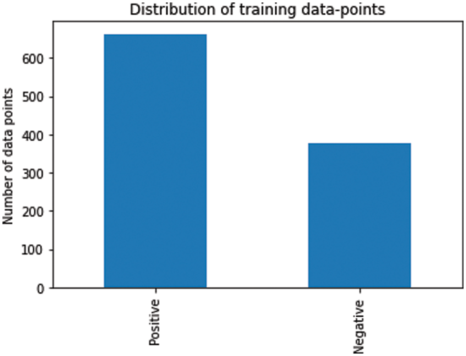
Figure 3: Class distribution of the training and validation datasets

2.3 Implementation Details

XLNet neural network model has been developed based on the Transformer-XL model [21]. XLNet model has been pretrained to learn bidirectional contexts using autoregressive (AR) method. Autoencoding and autoregressive modeling have been highly successful in natural language processing modeling. Autoregressive language modeling as the name suggests estimates the probability distribution of the text corpora using autoregressive model. AR language modeling is unidirectional and either tries to encode in forward context or backward context. Autoencoding based pretraining (such as BERT) uses the corrupted input to reconstruct the original data. It applies masking by replacing a portion of the tokens during the training process to recover the original tokens from the corrupted input. XLNet combines both the approaches and avoids the limitations of both and the produces a generalized autoregressive method.

There are many transfer learning model such as BERT, RoBERTa, XLNet etc. The reason for selecting XLnet over the other is that it has a similar structure to BERT and uses the Transformer-XL performance measure. The major advantage of XLNet over the BERT and RoBERTa is that it combines Auto-aggressive and bidirectional style. XLNet outperforms BERT and is comparable to RoBERTa [22]. The transfer learning model for the experiment was implemented on the Google Collaboratory platform using Python 3. The platform uses the Google Compute Engine backend (GPU) with 12.68 GB of RAM and 80 GB of disk space. The XLNet, pre-trained model is used as the base transfer learning model. XLNet is a BERT-like transfer learning model introduced by Google in 2019. The earlier transfer learning models had an issue with capturing bidirectional context because of the auto-encoding limitation. XLNet uses Permutation Language Modelling (PLM) that complements more features that overcome the earlier limitations and can capture bidirectional context. The pre-trained XLNet network model that has been used for this experiment is XLNet For Sequence Classification. For XLNet For Sequence Classification, the top of the pooled output of the XLNet model has been configured with a regression/sequence classification head. The network is optimized with the Adam optimizer algorithm with a weight decay (usually known as AdamW) of 0.01. The base learning rate was set to 2e-5. Though several optimizers such as RMSprop, Stochastic Descent Gradient, etc. have been tested with different values of the hyperparameters, AdamW produced more consistent results during multiple executions. The batch size for fine-tuning was set to 16 responses to avoid memory-related issues. XLNet requires a fixed-length input. Therefore, the maximum length of the input was set to 128 characters. Therefore, as the input sentences are of different lengths, padding and truncating were applied to all the inputs to get the same-size sentences. The sentences, which were longer than 128 characters, were truncated to their maximum length, and the remaining data from the longer sentences was discarded. The shorter sentences (shorter than 128 characters) were padded with zeros at the ends of the sentences until all the shorter sentences had a length equal to the maximum length. An XLNet tokenizer was used to convert all the text tokens into a sequence of integers (input ids) utilizing the XLNet tokenizer vocabulary. For the tokens that are followed by zeros, an attention mask of 1s was created.

The proposed approach has a training phase and a validation phase. During fine-tuning, the following operations were performed for each pass for training and evaluation/validation:

Training Process:

•   Computing the gradients in model training mode.

•   Unpacking the labels and data.

•   Using GPU for acceleration.

•   Clearing the previous pass’ gradients. (PyTorch accumulate gradients by default, that are good in RNNs but we need to clear them out here).

•   Feed the input data to the network in a Forward pass.

•   Using backpropagation in Backward pass.

•   Updating network parameters with optimizer.step().

•   Monitoring progress by tracking the variables.

Evolution Process:

•   Computing gradients for the model in evaluation mode.

•   Unpacking the labels and data.

•   Using GPU for acceleration.

•   Feed the input data to the network in a Forward pass.

•   Using validation data for computing loss and monitoring progress by tracking the variables.

The findings of the experiments are presented in the Section 3.

3  Results

We first give the training dataset findings in this section before moving on to the test dataset assessment results.

3.1 Training Results

Experiments were conducted with different values of the hyperparameters and with different optimizers. However, the network has produced the most consistent results with the AdamW optimizer algorithm with weight decay. The training was conducted for 15 epochs. Table 1 and Fig. 4 demonstrate the training loss for each epoch.

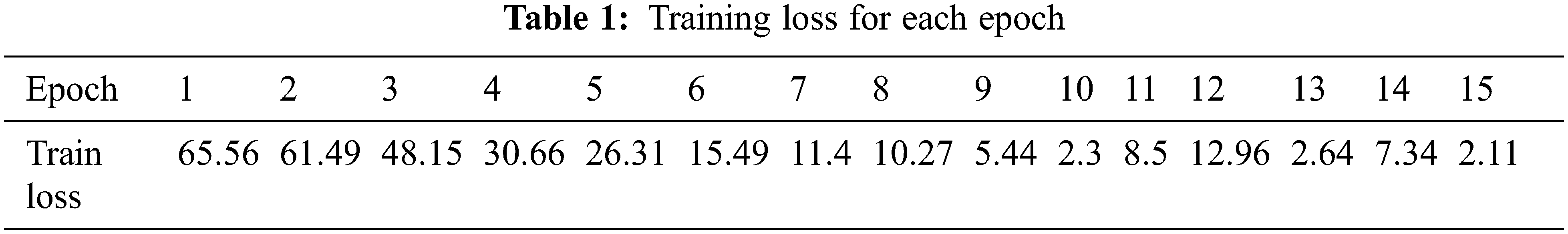
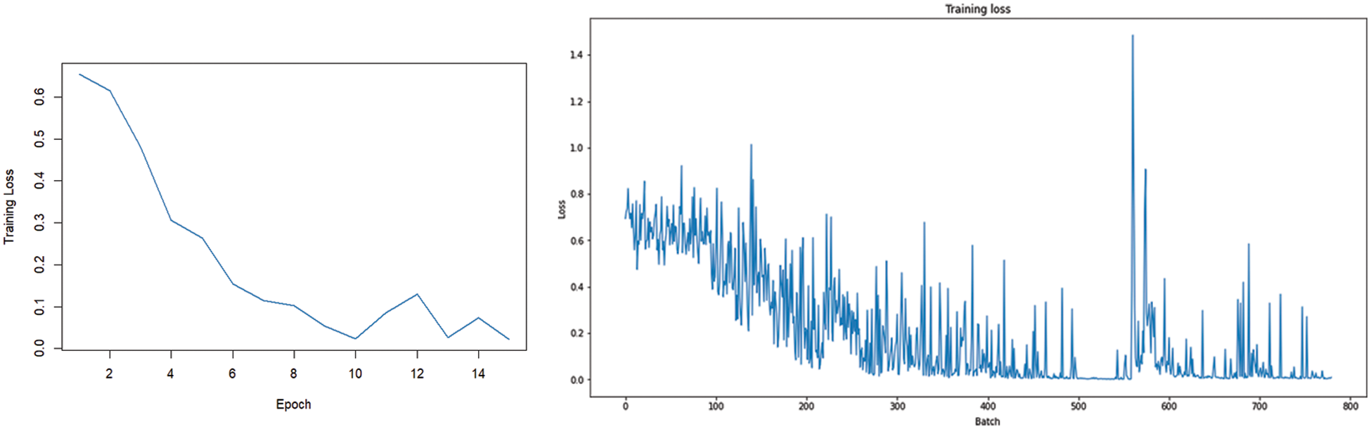
Figure 4: Training loss for each epoch

The batch size for fine-tuning was set to 16 responses to avoid memory-related issues. Fig. 4 illustrates the training loss for each batch. As the training reaches its final epochs, the training loss becomes almost zero for all the batches.

Table 2 and Fig. 5 demonstrate the validation accuracy across different epochs during the training process. The overall accuracy for the dataset is calculated for each epoch and presented in the following table and figure. During the initial phase of fine-tuning, a lower accuracy was achieved. However, as the training progressed, the model achieved almost 90% accuracy, which became almost constant in the last three epochs as shown in Figs. 5.

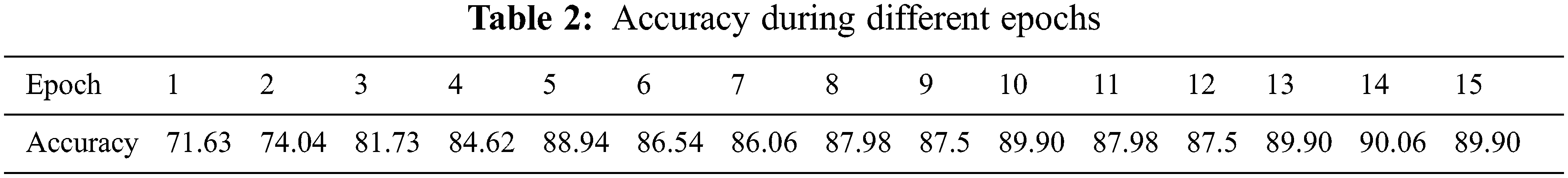
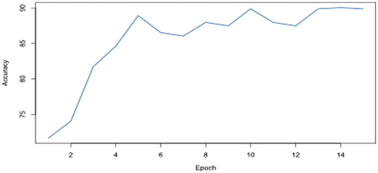
Figure 5: Accuracy during different epochs

3.2 Evaluation of Test Results

A dataset of 150 sentences was allocated as test data. The test dataset consists of 81 instances of the positive class and 69 instances of the negative class. Fig. 6 illustrates the class distribution of the test dataset.

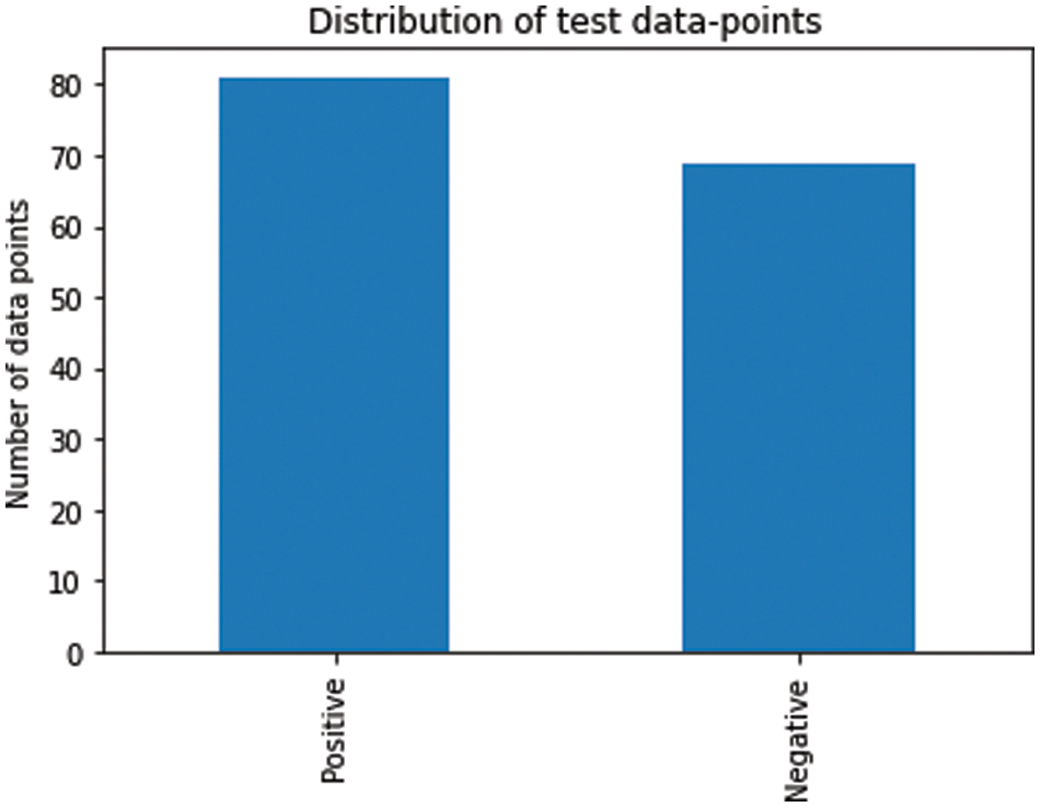
Figure 6: Class distribution of the testing dataset

4  Discussion

Several performance measures have been used to evaluate the performance of the sentiment classification model. Therefore, as there are only two classes based on the survey data collected, a, binary classification matrix such as Matthews’s correlation coefficient [23] can also be utilized for performance measures. To evaluate the performance of a classification model, N × N confusion matrix is used. Where N is the number of the target classes on the vertical axis and the predicted classes on the horizontal axis.

4.1 Confusion Matrix

Fig. 7 illustrates the confusion matrix based on the proposed test dataset. The confusion matrix represents the number of instances that have been classified accurately and incorrectly. It illustrates the number of instances of true positives (TP), true negatives (TN), false negatives (FN), and false positives (FP). As it is evident from the confusion matrix, 63 of 69 negative instances have been classified accurately in the negative class while 6 have been misclassified. For the positive class, 75 of 81 positive sentences have been classified accurately, and the remaining 6 sentences have been misclassified. This section evaluates and presents the various performance measures such as accuracy, precision, recall, F1 score, and Matthews’ correlation coefficient for the developed model.

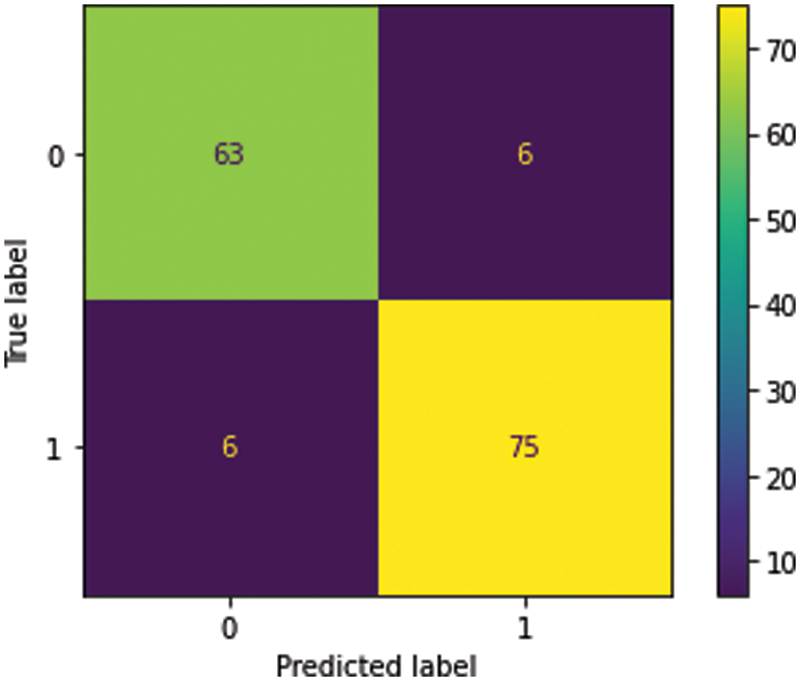
Figure 7: Confusion matrix for the test dataset

4.2 Accuracy

Accuracy is one of the principal performance evaluation matrixes to measure the performance of classification models. It is a measure of the total correct predictions out of the total number of predictions (including incorrect predictions). It can be defined as:

Accuracy= True Positive + True NegativeTotal Predictions (1)

Based on the random testing data, the proposed model has yielded an accuracy of 92%.

4.3 Precision

Positive predictive value or precision measures the performance of the classification model for accurately predicting the instances of the positive class against the total number of positive predictions. Mathematically it is represented as:

Precision= True PositiveTrue Positive + False Positive   (2)

The proposed model has scored 92.59% precision for the positive class.

4.4 Recall

For binary classification, recall can also be referred to as sensitivity. Recall measures the true positive rate and is evaluated as the ratio of the number of true positive predictions over the number of instances of the positive class used in the testing dataset. Mathematically, recall can be represented as:

Recall= True PositiveTrue Positive + False Negitive   (3)

The sensitivity or recall calculated for the proposed model is 92.59%. Fig. 8 represents the precision and recall curve of the proposed model.

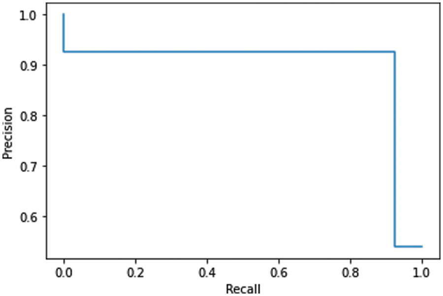
Figure 8: The precision and recall curve of the proposed model

4.5 F1-Score

The precision and the recall matrix primarily focus on true positives. However, it is important to consider the true negatives as well. The F1-score, also known as the F-measure, reflects the importance of both in binary classification and uses the harmonic mean of the two matrices (precision and recall). Mathematically, it is represented as:

F1−score= 2 ∗ Precision∗RecallPrecision + Recall (4)

F1–score measured for the proposed model is 92.56%.

4.6 Matthew’s Correlation Coefficient

Matthew’s correlation coefficient, hereafter referred to as MCC (Matthews, 1975) is used to measure the correlation between the predicted and actual classes of the binary classification. MCC is a more robust performance measure as compared to recall, precision, and F1-score because it takes all the entities of the confusion matrix into account [24,25]. MCC is defined as:

MCC=Cov(t,p)σt.σp= TP.TN−FP.FN(TP+FP)(TN+FN)(TP+FN)(TN+FP)   (5)

where, Cov(t,p) is the covariance between the actual classes of the cases and the predicted labels, (σp) is the standard deviation of the predicted classes and, ( σt ) is the standard deviation of the true classes.

Matthew’s correlation coefficient (MCC) has been evaluated at 0.84. The range of the MCC is between +1 and −1. A value close to +1 represents a direct correlation and signifies a better-quality model.

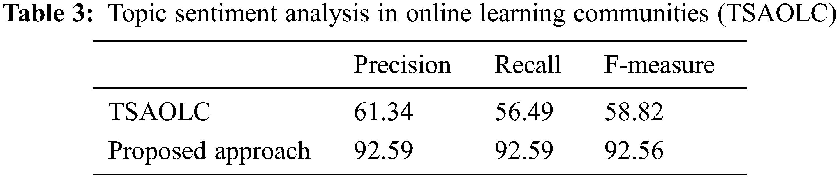
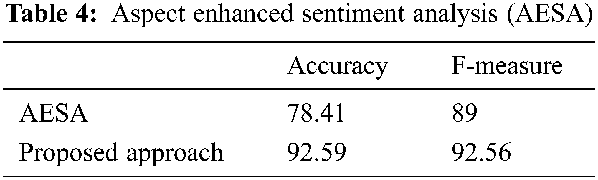
The paper’s experimental results are compared to the other approaches proposed in Aspect Enhanced Sentiment Analysis (AESA) by [26] and Topic Sentiment Analysis in Online Learning Communities (TSAOLC) by [27]. The results on the accuracy, precision, recall, and F-measure computed by our approach presented in our paper are better as compared to AESA and TSAOLC as shown in Tables 3 and 4.

5  Conclusions

This paper attempts to get a real understanding of the learners’ emotions about the learning process. A questionnaire has been designed and developed. This is to comprehend and analyze shortfalls in the areas related to imparting quality education. It uses XLNet to build a sentiment classification model to be utilized in its transfer learning methodology. XLNet has an advantage over BERT and RoBERTa in that it combines auto aggressive and bidirectional styles. The model was optimized with the Adam optimizer algorithm with a weight decay (usually known as AdamW). Based on the obtained results, it is observed that the proposed model accuracy yielded is 92% based on the random testing data. Also, the model has scored 92.59% precision for the positive class, and 92.59% is its sensitivity or recall. The F1–score has been measured at 92.56%, whereas Matthew’s correlation coefficient (MCC) has been evaluated at 0.84. When compared against the AESA and TSAOLC models, the proposed approach performs better in identifying the learners’ sentiments.

Acknowledgement: The authors extend their appreciation to the Deanship of Scientific Research at Saudi Electronic University for funding this research work through project number (8141).

Funding Statement: The authors extend their appreciation to the Deanship of Scientific Research at Saudi Electronic University for funding this research work through project number (8141).

Conflicts of Interest: The authors declare that they have no conflicts of interest to report regarding the present study.

References

1. B. Liu, “Many facets of sentiment analysis,” In: E. Cambria, D. Das, S. Bandyopadhyay and A. Feraco (eds.A Practical Guide to Sentiment Analysis. Socio-Affective Computing, vol. 5. Springer, Cham, Springer, pp. 11–39, 2017. [Google Scholar]
2. S. Thrun and L. Pratt, “Learning to learn: Introduction and overview,” in Learning to Learn, Boston, MA: Springer, pp. 3–17, 1998. [Google Scholar]
3. R. Caruana, “Multitask learning,” Machine learning, vol. 28, no. 1, pp. 41–75, 1997. [Google Scholar]
4. E. L. Thorndike, The fundamentals of learning. New York: Teachers College Press, 1932. [Google Scholar]
5. S. J. Pan and Q. Yang, “A survey on transfer learning,” IEEE Transactions on Knowledge and Data Engineering, vol. 22, no. 10, pp. 1345–1359, 2009. [Google Scholar]
6. K. Weiss, T. M. Khoshgoftaar and D. Wang, “A survey of transfer learning,” Journal of Big data, vol. 3, no. 1, pp. 1–40, 2016. [Google Scholar]
7. H. Guo, X. Zhuang, P. Chen, N. Alajlan and T. Rabczuk, “Analysis of three-dimensional potential problems in non-homogeneous media with physics-informed deep collocation method using material transfer learning and sensitivity analysis,” Engineering with Computers, vol. 313, no. 5786, pp. 1–22, 2022. [Google Scholar]
8. J. Zhou, S. Pan, I. Tsang and Y. Yan, “Hybrid heterogeneous transfer learning through deep learning,” Proceedings of the AAAI Conference on Artificial Intelligence, vol. 28, no. 1, pp. 2213–2219, 2014. [Google Scholar]
9. F. Zhuang, Z. Qi, K. Duan, D. Xi, Y. Zhu et al., “A comprehensive survey on transfer learning,” Proceedings of the IEEE, vol. 109, no. 1, pp. 43–76, 2020. [Google Scholar]
10. O. Day and T. M. Khoshgoftaar, “A survey on heterogeneous transfer learning,” Journal of Big Data, vol. 4, no. 1, pp. 29, 2017. [Google Scholar]
11. E. Bataa and J. Wu, “An investigation of transfer learning-based sentiment analysis in Japanese,” arXiv Preprint arXiv:1905.09642, 2019. [Google Scholar]
12. J. Devlin, M. W. Chang, K. Lee and K. Toutanova, “Bert: Pre-training of deep bidirectional transformers for language understanding,” arXiv Preprint arXiv:1810.04805, 2018. [Google Scholar]
13. N. Kirielle, P. Christen and T. Ranbaduge, “TransER: Homogeneous transfer learning for entity resolution,” in Proc. of the 25th Int. Conf. on Extending Database Technology (EDBT), 29th March-1st April (EDBTEdinburgh, pp. 118–130, 2022. [Google Scholar]
14. A. Farahani, B. Pourshojae, K. Rasheed and H. Arabnia, “A concise review of transfer learning,” in Proc. of the 2020 Int. Conf. on Computational Science and Computational Intelligence (CSCI), Las Vegas, NV, USA, pp. 344–351, 2020. [Google Scholar]
15. H. Daumé III, “Bayesian multitask learning with latent hierarchies,” arXiv preprint arXiv:0907.0783, 2009. [Google Scholar]
16. J. Pan, “Feature-based transfer learning with real-world applications,” PhD thesis, Hong Kong University of Science and Technology, Hong Kong, 2010. [Google Scholar]
17. K. Khalil, U. Asgher and Y. Ayaz, “Novel fNIRS study on homogeneous symmetric feature-based transfer learning for brain-computer interface,” Scientific Reports, vol. 12, no. 1, pp. 3198, 2022. [Google Scholar] [PubMed]
18. A. Soni, “Application and analysis of transfer learning-survey,” International Journal of Scientific Research and Engineering Development, vol. 1, no. 2, pp. 272–278, 2018. [Google Scholar]
19. J. He, C. Zhou, X. Ma, T. Berg-Kirkpatrick and G. Neubig, “Towards a unified view of parameter-efficient transfer learning,” (arXiv:2110.04366). arXiv. http://arxiv.org/abs/2110.04366, 2022. [Google Scholar]
20. W. Li, R. Zhao and X. Wang, “Human reidentification with transferred metric learning,” in Asian Conf. on Computer Vision, Berlin, Heidelberg, Springer, pp. 31–44, 2012. [Google Scholar]
21. Z. Yang, Z. Dai, Y. Yang, J. Carbonell, R. Salakhutdinov et al., “XLNet: Generalized autoregressive pretraining for language understanding,” in 33rd Conf. on Neural Information Processing Systems (NeurIPS 2019), Vancouver, Canada, pp. 1–18, 2019. [Google Scholar]
22. A. F. Adoma, N. M. Henry and W. Chen, “Comparative analyses of bert, roberta, distilbert, and xlnet for text-based emotion recognition,” in 2020 17th Int. Computer Conf. on Wavelet Active Media Technology and Information Processing (ICCWAMTIPIEEE, Chengdu, China, pp. 117–121, 2020. [Google Scholar]
23. B. W. Matthews, “Comparison of the predicted and observed secondary structure of T4 phage lysozyme,” Biochimica et Biophysica Acta (BBA)–Protein Structure, vol. 405, no. 2, pp. 442–451, 1975. [Google Scholar]
24. D. Chicco and G. Jurman, “The advantages of the Matthews correlation coefficient (MCC) over F1 score and accuracy in binary classification evaluation,” BMC Genomics, vol. 21, no. 1, pp. 1–13, 2020. [Google Scholar]
25. S. Khan, A. Alourani, B. Mishra, A. Ali and M. Kamal, “Developing a credit card fraud detection model using machine learning,” Approaches International Journal of Advanced Computer Science and Applications (IJACSA), vol. 13, no. 3, pp. 411–418, 2022. [Google Scholar]
26. J. Tao and X. Fang, “Toward multi-label sentiment analysis: A transfer learning based approach,” Journal of Big Data, vol. 7, no. 1, pp. 1–26, 2020. [Google Scholar]
27. K. Wang and Y. Zhang, “Topic sentiment analysis in online learning community from college students,” Journal of Data and Information Science, vol. 5, no. 2, pp. 33–61, 2020. [Google Scholar]
Cite This Article
Copyright © 2023 The Author(s). Published by Tech Science Press.
This work is licensed under a Creative Commons Attribution 4.0 International License , which permits unrestricted use, distribution, and reproduction in any medium, provided the original work is properly cited.
Downloads
Citation Tools