Coordinated Scheduling of Two-Agent Production and Transportation Based on Non-Cooperative Game

1  Introduction

In modern manufacturing models, various production connections inside a business or distinct clients outside a firm will have different personalized wants and compete for production resources. At this time, cooperative planning and decision-making among different decision makers must be considered [1]. Agnetis et al. [2] studied this sort of problem and proposed multi-agent production scheduling by viewing production links or customers as agents. Multi-agent production scheduling refers to multiple agents competing for the use of the common machines to process their respective jobs so that the objective of depending on the completion time of their own jobs is optimal [3,4]. In a distributed manufacturing environment, manufacturing equipments and individual agents may be in various geographical locations, and the manufacturing capacity of resources should be taken into account together with the synergy between transportation and production. The coordination of production and transportation is common in steel manufacturing, automotive sector suppliers and other industries [5–8].

Examples involving two-agent production and transportation may be found in the steel plant manufacturing process. As one practical example, the steelmaking-continuous casting processes in the steel plant demonstrate the real production settings. The manufacturing process is depicted in Fig. 1. The crude steel produced in the converter is refined and converted into liquid steel, which is transported to the continuous casting machine through transport vehicles. The molten steel can take two alternative modes according to the desired ingot shape in the ingot formation process. One is the mould casting mode that the molten steel in a ladle is poured into molds to solidify cylindrically-shaped ingots. The other is the continuous-casting mode that the molten steel is cast and cooled to form slabs, blooms or billets in the continuous caster. Due to the differences between the mould casting mode and the continuous-casting mode, they are regarded as two agents competing for the refined molten steel. The purpose is to schedule all of the jobs of both agents such that each agent’s objects are optimized.

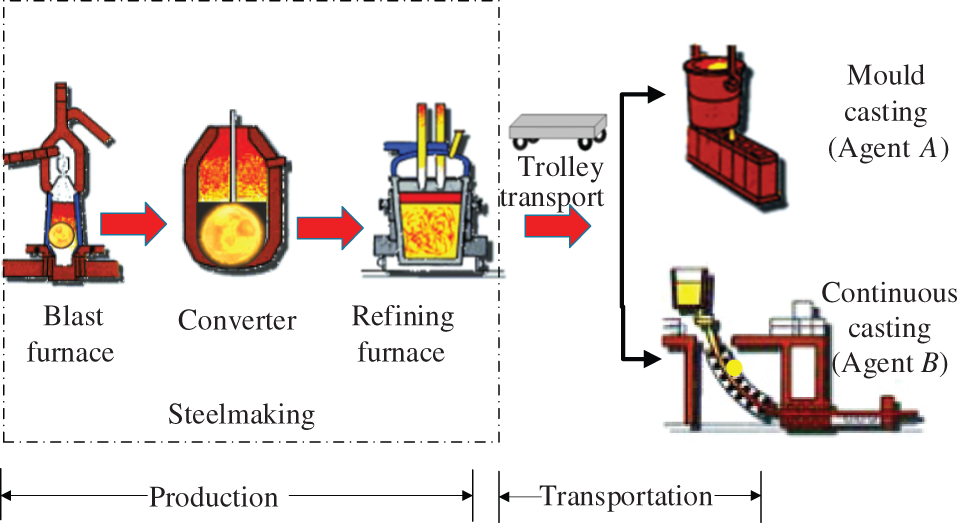
Figure 1: Steelmaking-continuous casting production process

The majority of research on multi-agent scheduling has been on a single machine. Baker et al. [9] and Agnetis et al. [10] studied the single-machine two-agent scheduling problem with the linear weighted sum model, the constrained optimization model, and the Pareto optimization model as objective functions. Liang et al. [11] studied the single-machine two-agent scheduling problem with release time and the makespan objective function, and established a mixed integer programming model. Wang et al. [12] described a multi-agent single-machine scheduling problem with release dates, where several packets (jobs) share a common network (processor) but are maintained by several competitive applications (agents) that optimize their criteria. The objective is to minimize the sum of the makespan belonging to several agents individually. Zhang et al. [13] extended the resource allocation fair pricing problem to single-machine two-agent scheduling, where the objectives of the two agents are the total number of tardy jobs and maximum cost, respectively. Furthermore, several researchers have studied multi-agent scheduling on parallel machines [14], batch machines [15,16] and flowshop [17].

There is less research on multi-agent scheduling issues that address transportation and processing cooperatively. Fan et al. [18] defined the objective function as the sum of the makespan and transportation time, and proposed a dynamic programming algorithm. Yin et al. [19] investigated a two-agent process and finished product batch transportation scheduling problem. A polynomial-time algorithm for minimizing the objective of agent A is given under the constraint that the objective of agent B does not exceed a given threshold. Qi et al. [20] showed that their algorithm is incorrect by a counterexample and presented polynomial-time algorithms to solve the problem in Yin et al. [19] in polynomial time.

In summary, the multi-agent scheduling problem is mostly studied as a two-agent scheduling problem under a single machine, with less consideration of the collaboration between processing and transportation. Most of the solution methods transform the multi-objective problem into a single-objective problem and solve the small-scale problem by an exact algorithm, ignoring the competitive relationship between two agents.

Mathematical programming approaches, meta-heuristic algorithms, intelligent optimization algorithms, and other methods are commonly adopted to solve the production scheduling problem [21,22]. Game theory takes into account the collaboration and competition between different subjects. Many researchers have adopted game theory to investigate the production scheduling problem. Zhou et al. [23] mapped each customer’s manufacturing task as a player, establishing a scheduling model and solving the Nash equilibrium point of the non-cooperative game model based on a hybrid adaptive genetic algorithm. Nong et al. [24] studied the scheduling problem of parallel batch machines with the objective of minimizing the makespan of each agent and mapping them to the player so as to build a game model. Zhang et al. [25] studied the real-time multi-objective flexible job shop scheduling problem and proposed a two-level scheduling method based on dynamic game theory to find the optimal solution through sub-game perfect Nash equilibrium. Wang et al. [26] constructed a game theory-based dynamic scheduling model for flexible job shop under emergency order addition, aiming at the rapidity and stability of the scheduling plan. Nie et al. [27] established a non-cooperative game model and proposed a game scheduling algorithm based on the genetic algorithm to solve the D-min Nash equilibrium, aiming at the shop scheduling problem in virtual manufacturing network and minimizing the makespan of all jobs.

It can be seen that more scholars have studied production scheduling problems based on non-cooperative games, although game theory is rarely applied to analyze multi-agent scheduling problems. As a result, non-cooperative game theory is used to investigate the two-agent production and transportation coordinated scheduling problem by taking into account the competition between the jobs of two agents for the processing sequence and transportation sequence from the standpoint of maximizing the payoff of agents.

This paper carries out the following three works listed below.

(1)   Two different production links or customers are regarded as agents in view of the competition for the same machine resources between the jobs from different production links or customers. After the job has been processed, it needs to be delivery to the respective agent, and the two agents have distinct objectives. Considering production and post-production transportation cooperatively, a scheduling problem of two-agent production and transportation coordination in a single machine is suggested.

(2)   A non-cooperative game model for the competition relationship between the jobs of two agents for the machine and the transport vehicle is constructed. The two agents are mapped as players, and the two agents compete for the processing position on the machine and the transportation position on the transport vehicle. The processing position and transportation position of the jobs are mapped as strategies, and the objective function of the two agents is mapped as payoff functions.

(3)   An approximate Nash equilibrium solution algorithm based on an improved genetic algorithm (NE-IGA) is proposed to solve the approximate Nash equilibrium solution of the problem. The fitness function is designed from the Nash equilibrium definition, and the genetic operator based on production and transportation is designed according to the characteristics of the two-agent production and transportation coordination scheduling problem in single-machine.

This paper is outlined as follows: Section 2 develops a non-cooperative game model to handle the problem of two-agent production transportation coordination scheduling in single machine. Section 3 designs an approximate Nash equilibrium solution method based on an improved genetic algorithm. Section 4 describes the experiment setting and the results of the experiment. Finally, Section 5 summarizes the conclusions.

2  A Non-Cooperative Game Model for Two-Agent Production and Transportation Scheduling in Single Machine

2.1 Problem Description

The jobs of two agents compete to be processed on a single machine and transported to their respective agents after completion, i.e., the jobs of two agents compete to get the order of processing on the machine and transport on the transport vehicle.

Let there be two agents: agent A and agent B, whose job sets are JA={J1A, …, JmA} , JB={Jm+1B, …, JnB} , and the total number of jobs is n. The number of jobs of agent A is m and the number of jobs of agent B is (n−m). The jobs of two agents compete for processing on a single machine, and the finished jobs on this machine need to be transported to agent A and agent B by a transport vehicle. The time for the transport vehicle to travel between machine and agent X is tX (X = A, B). The processing time of the Ji (i = 1, …, n) is Pi, the completion time is Ci. The finish time of the transport vehicle transporting the Ji is Ti, and the finish time Ti is defined as the time for the vehicle to transport Ji to the corresponding agent and back to the machine. Related parameters and variables are shown in Table 1.

Assume that the following assumptions are satisfied to simplify the problem.

(1)   The single machine can process continuously without the requirement for setup or switching time.

(2)   All jobs have arrived at the initial time and are ready to be processed.

(3)   The transport vehicle has a capacity restriction, and only one job can be loaded onto the transport vehicle at a time.

Considering that there is a competitive relationship between the two agents, each agent needs to maximize its own utility. The objective of agent A is the sum of the makespan and the total transportation time, while the objective of agent B is the sum of the total completion time and the total transportation time, as shown in Eqs. (1)–(2).

Minf1=maxi=1,2,..,m⁡{Ci}+mtA+∑i=1m−1Wi (1)

Minf2=∑i=m+1nCi+(n−m)tB+∑i=m+1n−1Wi (2)

where Wi denotes the waiting time for the transport vehicle to transport Ji. If Ji has finished processing when the transport vehicle has finished transporting the last job and returned to the machine, the transport vehicle does not need to wait, i.e., Wi = 0; if Ji has not finished processing when it returns to the machine, the transport vehicle needs to wait for Ji to finish processing, and the waiting time is the completion time of Ji minus the finish time of the previous transport job l, i.e., Wi = Ci − Tl .

According to the extended three-domain representation α | β | γ1, γ2 to describe the two-agent problem, α and β denote the characteristics of the machine environment and job, ri denotes the arrival time of Ji, and if all jobs arrive at the same time, then ri = 0. γ1, γ2 denotes denote the objective functions of the two agents, respectively. So the two-agent production and transportation coordination scheduling problem in a single-machine environment can be expressed as 1 | ri = 0 | f1, f2.

2.2 Non-Cooperative Game Model

In a non-cooperative game model, multiple players choose their strategies based on their own interests, and there is both conflict and cooperation between players, which conforms to the competition and cooperation between two agents for resources in the two-agent scheduling problem. As a result, we adopt non-cooperative game theory to address the problem of two-agent production and transportation scheduling in a single machine.

In a single machine setting, a non-cooperative game model for the two-agent production and transportation coordinated scheduling problem is established. The model can be formulated as Eq. (3).

G={I, S, U} (3)

where I denotes the number of game players. S = {S1, …, Sk} denotes the strategy of players, where So denotes the strategy of the players o(o = 1, 2,…, k). U = {U1 ,…,Uk} denotes the payoff function of player with respect to the strategy, where Uo denotes the payoff of the players o under the strategy.

Player: The jobs of the two agents fight for the sequence of processing on the machine and transit on the transport vehicle. The two agents are mapped as players.

Strategy: The strategy is defined as S = {S1, S2}, which is the set of actions or decision choices of the players. Each agent is responsible for two decisions: the processing position and transportation position of each job. Then the strategies of the two agents are as Eq. (4).

S1=(Mi,lA, Ti,jA)i=1, 2, …, m l, j∈nS2=(Mi,lB, Ti,jB)i=m+1, …, n l, j∈n (4)

where Mi,lA denotes that JiA is processed at location l, Ti,jA denotes that JiA is transported at trip j. Mi,lB denotes that JiB is processed at location l, and Ti,jB denotes that JiB is transported at trip j.

Not all strategies are valid. Strategy S is invalid when the following conditions occur.

(1)   Sequences of processing conflict: Because the two players only consider their own strategies, there will be two jobs processed at the same position, rendering the strategy invalid. In other words, for any two different jobs i1 and i2 in strategy S, the strategy is invalid when there is Mi1,lA=Mi2,lA or Mi1,lA=Mi2,lB .

(2)   Sequences of transport conflict: When two jobs are transported at the same position, the strategy is invalid. In other words, or any two different jobs i1 and i2 in strategy S, the strategy is invalid when there is Ti1,jA=Ti2,jA or Ti1,jA=Ti2,jB .

For example, the job sets of agent A and agent B are {J1, J2} and {J3}, respectively. Then, without considering conflicts, there are 3 processing positions and 3 transport positions from which all jobs can choose on the machine or vehicle, resulting in 33 × 33 × 33 = 729 different strategies, but some of them are invalid. For example, strategy S1 = {(2, 2), (1, 1)}, S2 = {(1, 3)}, where the J2A and J1B are processed at the same position, so the strategy is invalid. Strategy S1 = {(2, 2), (1, 1)}, S2 = {(3, 2)}, the J1A and J1B are transported at the same position, making this strategy invalid as well. After deleting all invalid strategies, there remained 36 feasible strategies.

Payoff function: The payoff function is the gain obtained by the game parties under the strategy. Therefore, for agent A and agent B under the strategy, the payoff function U = {U1, U2}. Taking the objective functions of the two agents as their payoff functions: U1 = f1, U2 = f2, the game model of the two-agent scheduling problem can be described as Eq. (5).

G={S1, S2; U1, U2} (5)

Nash equilibrium: In the non-cooperative game model, there exists a certain strategy S* = {S1*, S2*}, satisfying the two game parties unilaterally changing their own strategies without increasing their own payoff, that is, the strategy S* is a Nash equilibrium solution when Eq. (6) is satisfied.

uo(So∗, S−o∗)≥uo(So, S−o∗) (6)

where uo denotes the payoff function of the game player o and S−o∗ denotes the combination of strategies of the game players other than the game player o.

For example, the job sets of agent A and agent B are {J1, J2} and {J3}, respectively, with the relevant parameters as shown in Table 2.

According to the non-cooperative game model built for the two-agent production and transportation coordination scheduling problem, there are 36 alternative strategies for agent A and 9 alternative strategies for agent B. According to the constructed payoff matrix, nine pure strategy Nash equilibriums can be obtained using the delineation method: S1 = {(1, 1), (2, 2); (3, 3)}, S2 = {(1, 3), (2, 1); (3, 2)}, S3 = {(1, 3), (2, 2); (3, 1)}, S4 = {(1, 1), (3, 2); (2, 3)}, S5 = {(1, 3), (3, 1); (2, 2)}, S6 = {(1, 3), (3, 2); (2, 1)}, S7 = {(2, 2), (3, 1); (1, 3)}, S8 = {(2, 3), (3, 1); (1, 2)}, S9 = {(3, 3),(2, 2); (1, 1)}, corresponding to the payoffs of (5.2, 6.3), (4.4, 9.5), (4.4, 9.5), (8.8, 4.3), (6.2, 6.5), (6.2, 6.5), (8.8, 5.2), (6.2, 8.5), (6.2, 5.5).

3  An Approximate Nash Equilibrium Solution Algorithm Based on an Improved Genetic Algorithm

The strategy space of the game model grows exponentially as the number of jobs of two agents increases, and the genetic algorithm can undertake a speedy search for the best solution without the limitation of scale change. Therefore, an approximate Nash equilibrium solution algorithm based on an improved genetic algorithm (NE-IGA) has been developed to seek the approximate Nash equilibrium of the provided game model.

3.1 Coding

According to the action strategy in the game model, integer coding is applied, and each job needs to choose a processing position and a transportation position, so each chromosome is divided into two sections, as shown in Fig. 2. The length of the chromosome is 2n, with the initial n bits representing the processing sequence and the latter n bits representing the transportation sequence, and each component representing the whole arrangement of n jobs.

Figure 2: Coding scheme

For example, there are 5 jobs with chromosome codes (3, 4, 1, 2, 5, 2, 5, 1, 3, 4), which implies that the processing sequence of the jobs is 3, 4, 1, 2, 5, namely J3→ J4→ J1→ J2→ J5, and the transportation sequence of the jobs is 2, 5, 1, 3, 4, namely J2→ J5→ J1→ J3→ J4.

3.2 Fitness Function

The design of the fitness function is critical to resolving the Nash equilibrium. The objective of the two-agent production and transportation coordination scheduling problem is to minimize the objective functions of agents A and B. According to the definition of Nash equilibrium in the non-cooperative game model, when the Nash equilibrium is reached, it is difficult for the players to improve their own payoffs by modifying their own strategies, and the payoffs of the two agents are close enough to the best payoffs of the previous generation. As a result, the Nash equilibrium is determined by the difference between individual payoffs in the current generation and the best individual payoff in the previous generation. Second, the genetic algorithm calculates the likelihood of individual inheritance to the next generation based on the proportion of individual fitness, which must be positive. The fitness function is defined as Eq. (7).

Fg⁡(U1g, U2g)=∑o=12|Uog−U~og−1| (7)

U~og−1=minq∈Q⁡{Uoqg−1} (8)

where U1g denotes the payoff of agent A at generation g; U2g denotes the payoff of agent B at generation g; U~1g−1 denotes the best payoff of agent A at generation g−1; U~2g−1 denotes the best payoff of agent B at generation g−1, and Q is the set of populations.

According to the definition of the Nash equilibrium of the non-cooperative game model, the smaller the fitness value, the better. Defining Eq. (7) satisfies Eq. (9) when the algorithm finds the Nash equilibrium.

|Uog−U~og−1|<ηoo=1, 2 (9)

where ηo is the threshold applied to determine the solution to the scheduling of the game model, i.e., the criterion for determining the Nash equilibrium, taken as a smaller positive number. To simplify the problem, we take η1 = η2 = η. Obviously, the Nash equilibrium threshold η determines the approximation degree between the solution obtained by the algorithm and the Nash equilibrium. If the value of η is too large, the approximation degree of the solution will be poor, while if the value of η is too small, the convergence time of the algorithm will be prolonged. Therefore, the results obtained by fast global search of the genetic algorithm approximate the Nash equilibrium.

3.3 Genetic Operator

3.3.1 Selection Operator

The roulette selection operator is applied, and the likelihood of each chromosome joining the next generation is equal to the ratio of its fitness value to the total fitness values of the whole population. Then, according to the single lottery logic, chromosomes are chosen based on the random number’s area.

The fitness is divided into Fg⁡(U1g, U2g) parts, with each individual accounting for 1/ Fg⁡(U1g, U2g) , and then the chromosomes are selected according to the region where the random numbers are located, according to the single draw logic.

3.3.2 Production and Transportation-Based Two-Point Cross Operator

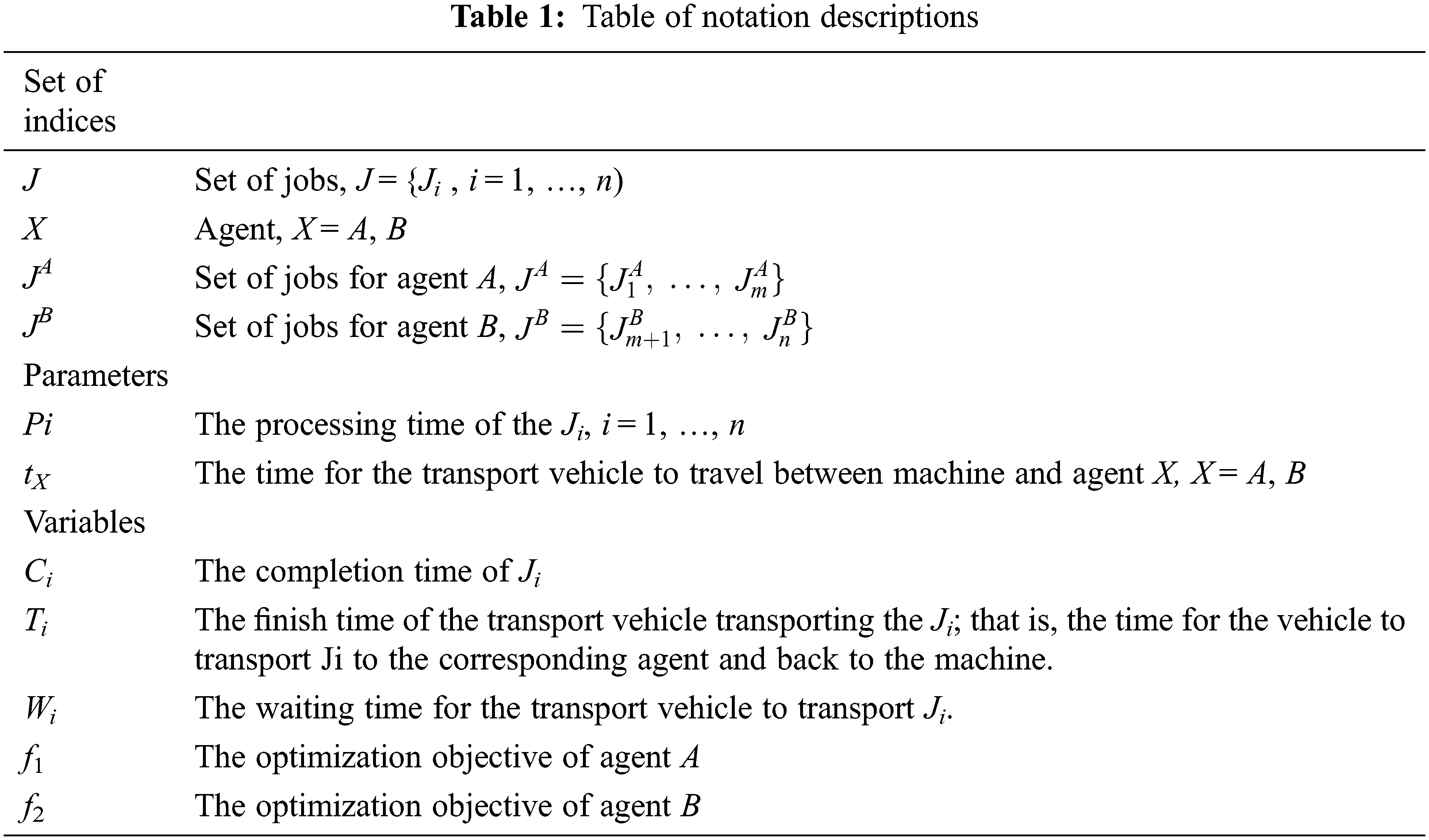
Paternal chromosomes y1 and y2 are chosen. Two gene loci are chosen at random from the first n production sequence of chromosome y1, and the matching two gene loci are chosen at random from the final n transport sequence and given to the offspring chromosome y. To avoid the formation of invalid chromosomes, offspring y is assigned from parent chromosome y2 in left-to-right order, with the exception of loci previously selected for chromosome y1. The crossover process is shown in Fig. 3.

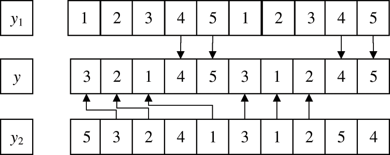
Figure 3: Production and transportation-based two-point crossover operation

3.3.3 Production and Transportation-Based Two-Point Mutation Operator

Chromosome y3 is chosen. To obtain the mutant chromosome y, two gene loci are randomly picked from the first n production loci of y3 for exchange, and two gene loci are randomly selected from the final n transport loci for exchange. The mutation process is shown in Fig. 4.

Figure 4: Production and transportation-based two-point mutation operation

Crossover or mutation operations are decided based on the similarity between parental chromosomes in order to improve population diversity and avoid slipping into a local optimum. The similarity between chromosomes y1 and y2 is expressed by the Hamming distance D(y1, y2). The smaller the D(y1, y2), the greater the difference between y1 and y2, and the greater the likelihood of obtaining new offspring chromosomes after crossover operation. The larger the D(y1, y2), the smaller the difference between y1 and y2 , and the crossover operation tends to leave the offspring chromosomes unchanged, and the mutation operation is employed at this time. To decide whether to do the mutation operation, according to the similarity relative percentage threshold φ. When the formula (10) is satisfied, the algorithm considers the similarity of the selected parent chromosome to be insufficient and executes the crossover operation. Otherwise, the selected parent chromosome’s resemblance is regarded as strong, and the mutation operation is carried out.

D(y1, y2)n≤φ (10)

where n is the number of jobs.

3.4 Algorithm Flow

The optimal individual retention strategy is adopted by NE-IGA to safeguard the best individuals in each generation of the population from being eliminated during subsequent selection, crossover, or mutation. This is accomplished by replacing the one with the largest value of the fitness function calculated in the offspring generation with the one with the smallest value of the fitness function in the parent generation.

The following are the steps of NE-IGA for solving the two-agent production and transportation coordination scheduling problem. And Fig. 5 depicts the algorithm flow.

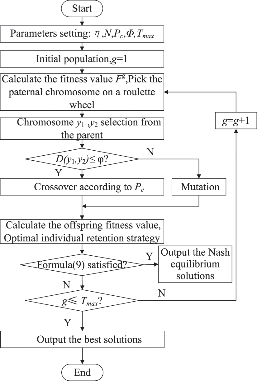
Figure 5: Algorithm flow chart

Step1: Parameter settings: population size N, crossover probability Pc, variation operation threshold φ and maximum number of iterations Tmax.

Step2: Initialize the population and set g = 1.

Step3: The fitness value Fg⁡(U1g, U2g) of each chromosome is calculated according to Eq. (7), and the parental chromosome is selected by roulette.

Step4: Update the population. Two chromosomes y1 and y2 are chosen at random from the parent generation, and the similarity is calculated to see if Eq. (10) is satisfied. If not, the mutation operation is performed. Otherwise, the crossover operation is performed according to the crossover probability Pc.

Step5: Retain the best individuals. Calculate the fitness value of the current population using Eq. (7). And replace the individuals with the worst fitness value in the offspring population with the best individuals in the parent population.

Step6: If Eq. (9) is met, it outputs the optimal solution, which is the approximate Nash equilibrium solution. Otherwise, proceed to Step 7.

Step7: Determine whether the maximum number of iterations has been reached, i.e., whether g = Tmax is true; if so, the optimal solution of this generation is output as the Nash equilibrium approximate solution to end the algorithm; otherwise, g = g+1, return to step 3.

4  Numerical Experimental Analysis

The following numerical example is created for simulation and analysis in order to validate the effectiveness of the proposed algorithm. The experiments are carried out on an Intel(R) Core(TM) i5-7200U CPU 2.50 GHz 2.71 GHz processor, 8 GB RAM, and Unity 2017 software.

4.1 Selection of Initial Circumstances and Parameters

Take m = 6 and n = 12, which means that agent A and agent B each have 6 jobs to process, while Pi and tx are chosen at random on the interval [1,10]. The following orthogonal experiments are aimed at determining the algorithm’s parameter selection. The population size N is set to 50, 100, and 200; the crossover probability Pc is set to 0.7, 0.8, and 0.9; the similarity threshold φ is set to 0.5, 0.6, and 0.7; and the Nash equilibrium threshold η is set to 0.01, 0.05, and 0.1. Nine groups of experimental data are produced at random, and the mean values of the objective functions of the two agents are determined for each group of data. The parameters are then determined by calculating the mean values of the objective functions over 9 groups of varied experimental data. Table 3 displays the results.

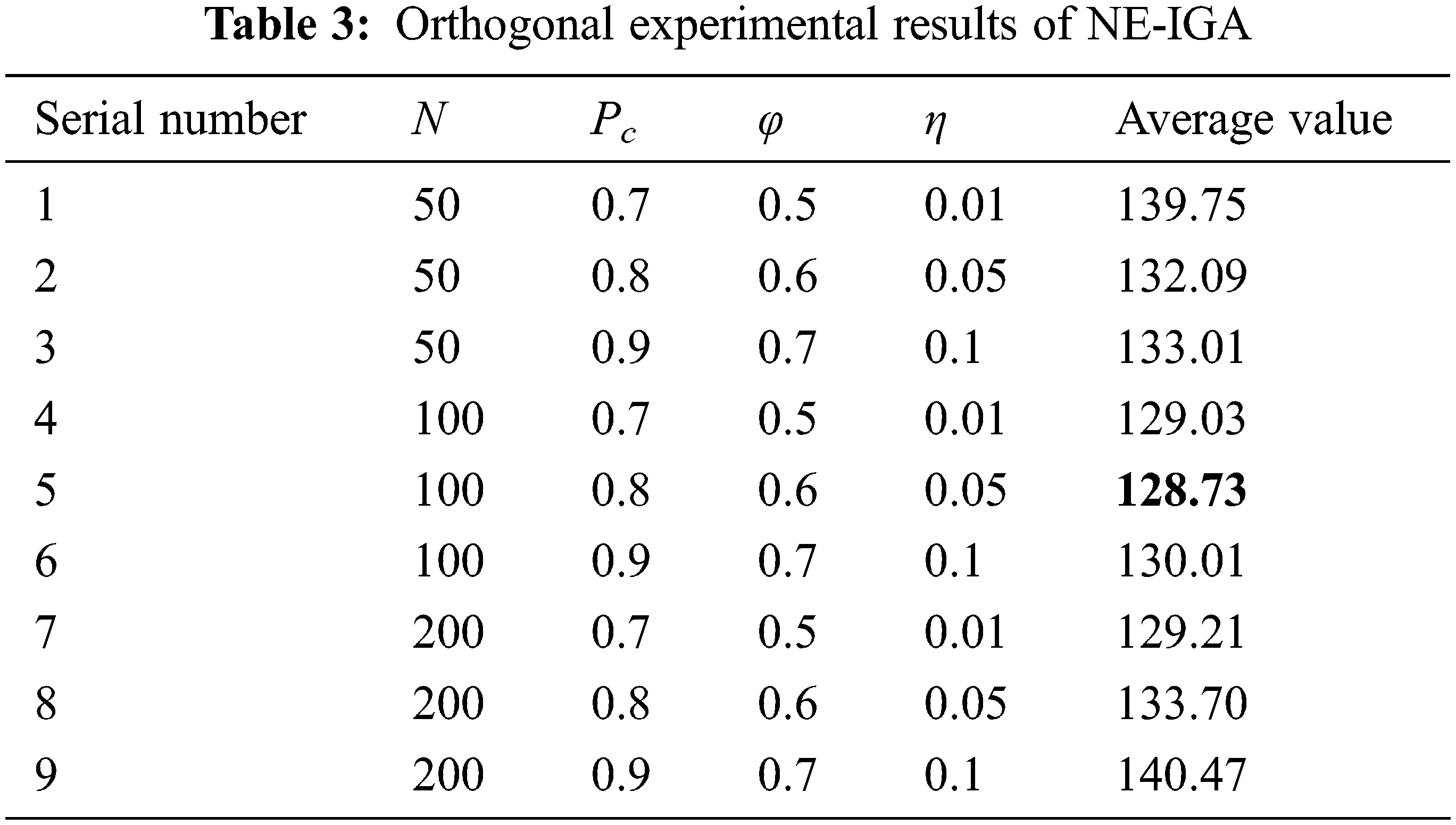
It can be seen from Table 3 that the fifth group has the smallest mean, so the population size N is determined to be 100, the crossover probability Pc is 0.8, the similarity threshold φ is 0.6, and the Nash equilibrium threshold η is 0.05.

Fig. 6 shows the convergence of the fitness function when the algorithm iterates to 500 generations with the above experimental parameters. It can be seen that the fitness function converges to the given threshold when the number of iterations is close to 400, and it has stabilized at this time. Therefore, the maximum number of iterations for this experiment is chosen to be 400.

Figure 6: The iterative convergence curve for the best fitness value

4.2 Analysis of Numerical Experimental Results

Fig. 7 shows the scheduling Gantt charts of the algorithm when it runs for the first, 100th, and 400th generations. Table 4 shows the scheduling schemes and the payoff of the two agents for the corresponding number of iterations. It can be seen that the objective function values of both agents A and B in the 400th iteration scheduling scheme are reduced when compared to the first and 100th iterations, and it is difficult to change the objective functions of both agents by unilaterally changing the positions of the artifacts at the 400th iteration.

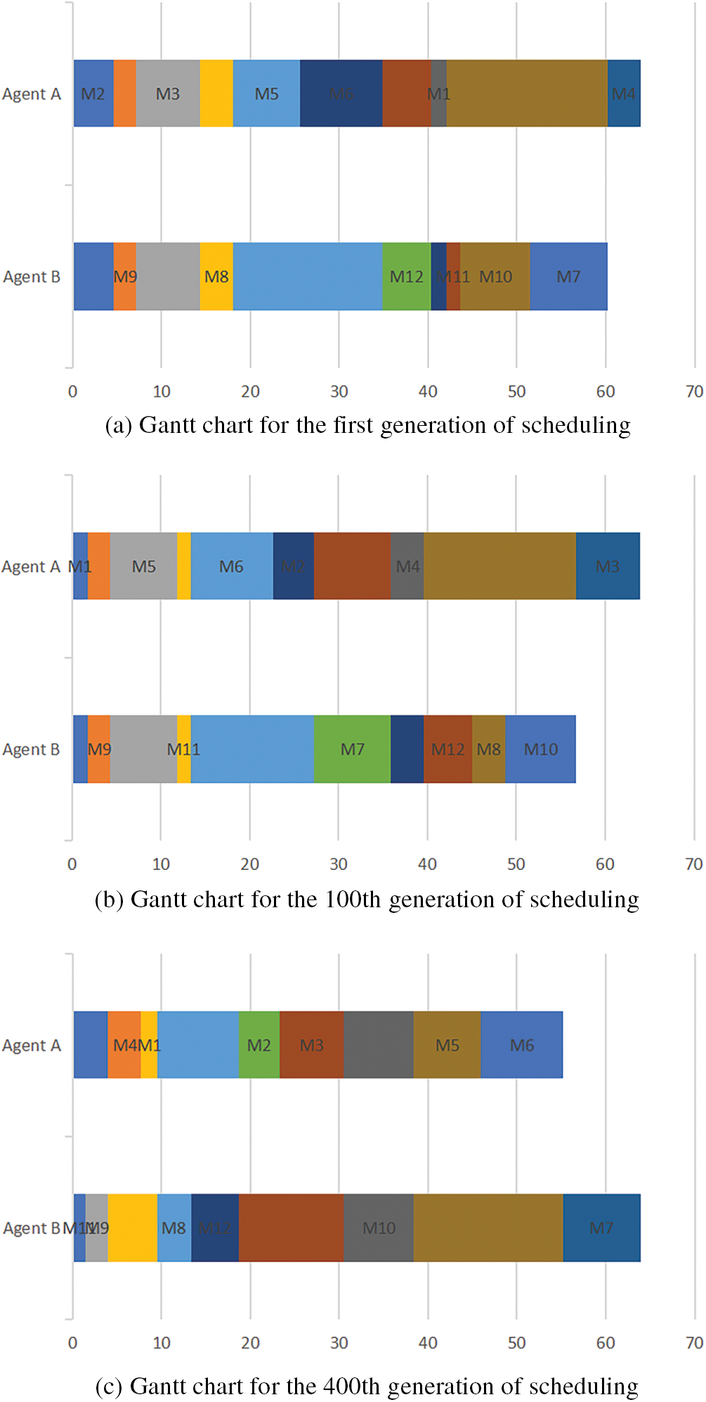
Figure 7: NE-IGA scheduling Gantt chart

4.3 Experimental Comparison

To further validate the efficacy of the proposed algorithm, a comparison analysis is done at various experimental sizes, utilizing the Longest Processing Time first (LPT) and the Shortest Processing Time first (SPT).

Fig. 8 and Table 5 illustrate the scheduling Gantt charts and payoff of the two agents for m = 6 and n = 12 under the LPT, SPT, and NE-IGA. It can be seen that the LPT rule has the worst payoff for agent A and agent B, and the scheduling plan is not reasonable. When compared to the other two rules, NE-IGA has a relatively superior payoff for both agent A and agent B, and the payoff for agent A and agent B is improved by 8.3% and 2.8% compared to SPT, and by 8.7% and 42.5% compared to the LPT rule. The average value of the two agents’ objective functions is improved by 34.3% and 4.6%, respectively, when compared to the LPT and SPT. As a result, the NE-IGA obtains a superior scheduling plan for both agent A and agent B.

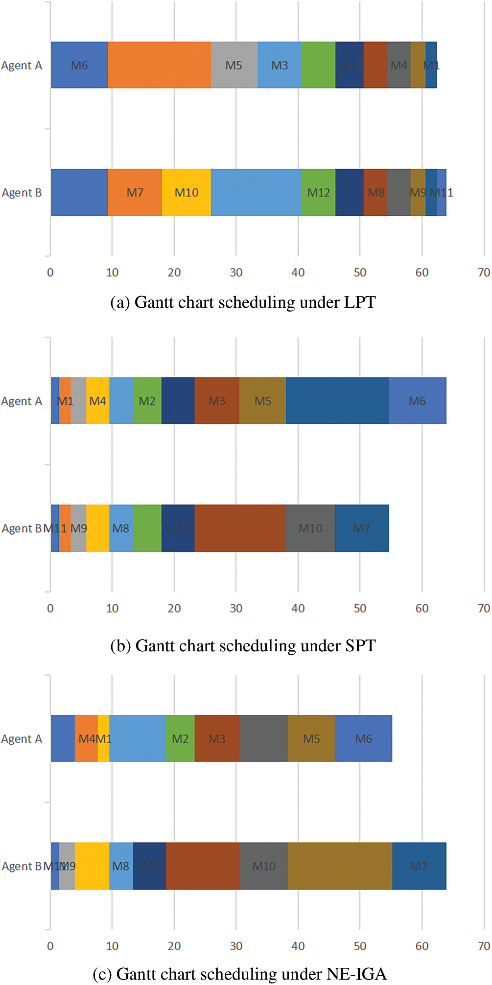
Figure 8: Gantt chart comparison of different algorithms when n = 12 and m = 6

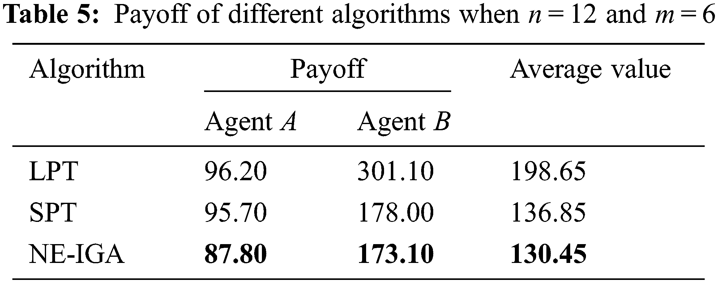
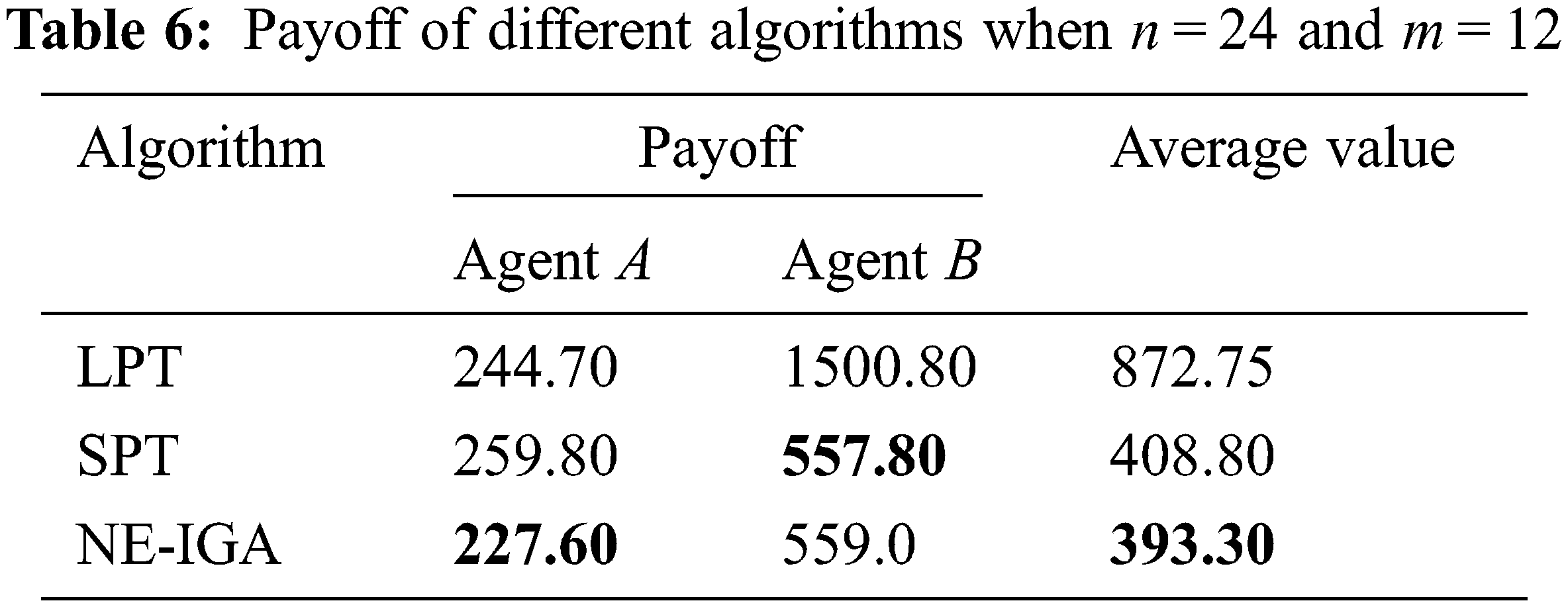
Table 6 compares the payoff of the NE-IGA to the LPT and SPT for two agents with m = 12 and n = 24. The payoff for agent B under the LPT rule is the worst, which is adverse for agent B, therefore the scheduling plan is not rational. Although the payoff of agent B is the best under the SPT, the payoff of agent A is the poorest at this moment, and the scheduling plan is likewise inappropriate. The payoff for both agent A and agent B under the NE-IGA is quite good when compared to the other two rules. The payoff of agent A is enhanced by 12.4% when compared to the SPT, while the payoffs of agents A and B are increased by 6.0% and 62.8%, respectively, when compared to the LPT. Furthermore, the average value of the objective function of both agents is the least under the NE-IGA, which is improved by 54.9% and 3.8%, respectively, over the LPT and SPT rules.

It can be seen that the objective functions of the two agents under the NE-IGA algorithm can converge to the optimum at the same time under different experimental scales, and a solution closer to the Nash equilibrium is obtained.

5  Conclusions

In this paper, we investigate the problem of coordinated production and transportation scheduling for two agents in a single machine. The jobs of two agents compete to be processed on a single machine and delivered to their respective agents after completion, and there is also competition for the transport vehicle. The objective of agent A is the sum of the makespan and the total transportation time, whereas the objective of agent B is the sum of the total completion time and the total transportation time. A non-cooperative game model is developed with two agents as players whose jobs fight for processing and transportation on the machine and vehicle; the processing and transportation position of the jobs as the game strategy; and the objective functions of the two agents as their payoff. The NE-IGA is meant to solve the approximate Nash equilibrium by designing the coding and genetic operators based on the processing and transportation sequence, as well as the fitness function based on the Nash equilibrium definition. The classic heuristic criteria are contrasted with simulation results at various experimental sizes. The experimental results show that the NE-IGA scheduling plan produces better results, with average performance improving by 44.6% and 4.2%, respectively, when compared to the LPT and SPT.

This paper assumes that the transport vehicle can only transport one job at a time and does not consider batch transport. Furthermore, the job may need to be delivered to the matching agent for the next processing within a limited time after the current machine processing is completed, which is known as the transportation waiting constraint. Therefore, the problem of two-agent production and transportation coordination scheduling considering transportation batch and transportation waiting time constraints can be further investigated in a single machine environment in the future. Furthermore, the development of new efficient algorithms is a potential research topic for the problem of two-agent production and transportation coordination.

Acknowledgement: The authors wish to acknowledge the contribution of Liaoning Key Lab of Equipment Manufacturing Engineering Management, Liaoning Research Base of Equipment Manufacturing Development, Liaoning Key Research Base of Humanities and Social Sciences: Research Center of Micro-management Theory of SUT.

Funding Statement: This work was supported in part by the Project of Liaoning BaiQianWan Talents Program under Grand No. 2021921089, the Science Research Foundation of Educational Department of Liaoning Province under Grand No. LJKQZ2021057 and WJGD2020001, the Key Program of Social Science Planning Foundation of Liaoning Province under Grant L21AGL017, the special project of SUT on serving local economic and social development decision-making under Grant FWDFGD2021019, the “Double First-Class” Construction Project in Liaoning Province under Grant ZDZRGD2020037.

Conflicts of Interest: The authors declare that they have no conflicts of interest to report regarding the present study.

References

1. M. M. E. Alemany, F. Alarcón, F. C. Lario and J. J. Boj, “An application to support the temporal and spatial distributed decision-making process in supply chain collaborative planning,” Computers in Industry, vol. 62, no. 5, pp. 519–540, 2011. [Google Scholar]

2. A. Agnetis, P. B. Mirchandani and D. Pacciarelli, “Nondominated schedules for a job-shop with two competing users,” Computational & Mathematical Organization Theory, vol. 6, no. 2, pp. 191–217, 2000. [Google Scholar]

3. O. J. Shukla, G. Soni and R. Kumar, “A review of multi agent-based production scheduling in manufacturing system,” Recent Patents on Engineering, vol. 15, no. 5, pp. 15–32, 2021. [Google Scholar]

4. Y. Q. Liu, S. D. Sun, X. V. Wang and L. H. Wang, “An iterative combinatorial auction mechanism for multi-agent parallel machine scheduling, ” International Journal of Production Research, vol. 60, no. 1, pp. 361–380, 2022. [Google Scholar]

5. E. Guzman, B. Andres and R. Poler, “A MILP model for reusable containers management in automotive plastic components supply chain,” in The Proc. of Working Conf. on Virtual Enterprises, Saint Etienne, France, pp. 170–178, 2021. [Google Scholar]

6. Z. Y. Zhao, S. Y. Li, S. X. Liu, S. Liu and Y. F. Zhao, “A review of dynamic scheduling in iron and steel production process,” Metallurgical Industry Automation, vol. 46, no. 2, pp. 65–79, 2022. [Google Scholar]

7. B. Andres, R. Sanchis, J. Lamothe, L. Saari and F. Hauser, “Integrated production-distribution planning optimization models: A review in collaborative networks context,” International Journal of Production Management and Engineering, vol. 5, no. 1, pp. 31–38, 2017. [Google Scholar]

8. B. Andres and R. Poler, “Models, guidelines and tools for the integration of collaborative processes in non-hierarchical manufacturing networks: A review,” International Journal of Computer Integrated Manufacturing, vol. 29, no. 2, pp. 166–201, 2016. [Google Scholar]

9. K. R. Baker and J. C. Smith, “A multiple-criterion model for machine scheduling,” Journal of Scheduling, vol. 6, no. 1, pp. 7–16, 2003. [Google Scholar]

10. A. Agnetis, P. B. Mirchandani and D. Pacciarelli, “Scheduling problems with two competing agents,” Operations Research, vol. 52, no. 2, pp. 229–242, 2004. [Google Scholar]

11. J. H. Liang, H. Y. Xue, D. Y. Bai and Y. H. Miao, “A branch and bound algorithm for the bi-agent single-machine scheduling problem with release dates,” Operations Research and Management Science, vol. 28, no. 10, pp. 83–88, 2019. [Google Scholar]

12. X. Y. Wang, T. Ren, D. Y. Bai, C. Ezeh, H. D. Zhang et al., “Minimizing the sum of makespan on multi-agent single-machine scheduling with release dates,” Swarm and Evolutionary Computation, vol. 69, pp. 100996–1–100996–19, 2022. [Google Scholar]

13. X. G. Zhang, J. Y. Liu and T. X. Cui, “Single machine KS fair pricing problem with two-agent based on the number of delayed jobs and the maximum cost function,” Journal of Chongqing Normal University (Natural Science), vol. 37, no. 1, pp. 16–21, 2020. [Google Scholar]

14. K. J. Zhao and X. W. Lu, “Two approximation algorithms for two-agent scheduling on parallel machines to minimize makespan,” Journal of Combinatorial Optimization, vol. 31, no. 1, pp. 260–278, 2016. [Google Scholar]

15. Q. Feng, W. P. Shang and C. W. Jiao, “Two-agent scheduling on a bounded parallel-batching machine with makespan and maximum lateness objectives,” Journal of the Operations Research Society of China, vol. 8, no. 1, pp. 189–196, 2020. [Google Scholar]

16. C. He and X. X. Han, “Two-agent scheduling on an unbounded parallel-batching machine to minimize maximum cost and makespan,” Operations Research Transactions, vol. 22, no. 3, pp. 109–116, 2018. [Google Scholar]

17. D. Y. Bai, A. Diabat, X. Y. Wang, D. D. Yang, Y. Fu et al., “Competitive bi-agent flowshop scheduling to minimise the weighted combination of makespans,” International Journal of Production Research, 2021. https://doi.org/10.1080/00207543.2021.1923854 [Google Scholar] [CrossRef]

18. J. Fan, “Integrated production and delivery scheduling problem with two competing agents,” in The Proc. of IEEE Int. Conf. on Advanced Management Science, Chengdu, China, pp. 157–160, 2010. [Google Scholar]

19. Y. Yin, Y. Wang, T. C. E. Cheng, D. Wang and C. C. Wu, “Two-agent single-machine scheduling to minimize the batch delivery cost,” Computers & Industrial Engineering, vol. 92, pp. 16–30, 2016. [Google Scholar]

20. X. L. Qi and J. J. Yuan, “A further study on two-agent scheduling on an unbounded serial-batch machine with batch delivery cost,” Computers & Industrial Engineering, vol. 111, pp. 458–462, 2017. [Google Scholar]

21. E. Guzman, B. Andres and R. Poler, “Models and algorithms for production planning, scheduling and sequencing problems: A holistic framework and a systematic review,” Journal of Industrial Information Integration, vol. 27, no. 5, pp. 100287, 2022. [Google Scholar]

22. J. Mula, M. Díaz-Madroñero, B. Andres, R. Poler and R. Sanchis, “A capacitated lot-sizing model with sequence-dependent setups, parallel machines and bi-part injection moulding,” Applied Mathematical Modelling, vol. 100, pp. 805–820, 2021. [Google Scholar]

23. G. H. Zhou, R. Wang, P. Y. Jiang and G. H. Zhang, “Non-cooperation game model and hybrid adaptive genetic algorithm for job-shop scheduling,” Journal of Xi’an Jiaotong University, vol. 44, no. 5, pp. 35–39, 2010. [Google Scholar]

24. Q. Q. Nong, S. J. Guo and L. H. Miao, “The shortest first coordination mechanism for a scheduling game with parallel-batching machine,” Journal of the Operations Research Society of China, vol. 4, no. 4, pp. 517–527, 2016. [Google Scholar]

25. Y. F. Zhang, J. Wang and Y. Liu, “Game theory based real-time multi-objective flexible job shop scheduling considering environmental impact,” Journal of Cleaner Production, vol. 167, pp. 665–679, 2017. [Google Scholar]

26. J. Wang, Y. J. Peng and G. H. Luo, “Non-cooperative game theory and RFID based integrating rush orders flexible shop floor dynamic scheduling method,” Manufacturing Technology and Machine Tools, no. 6, pp. 164–170, 2018. [Google Scholar]

27. L. Nie, G. H. Zhang, X. G. Wang and Y. W. Bai, “A Game-theory based optimization approach for job scheduling in virtual manufacturing network,” China Mechanical Engineering, vol. 30, no. 12, pp. 1492–1497, 2019. [Google Scholar]