Dynamic Allocation of Manufacturing Tasks and Resources in Shared Manufacturing

1  Introduction

With the advancements in information and computer technologies, the manufacturing industry has been undergoing a transformation from digital manufacturing to intelligent manufacturing. Particularly in recent years, the advent of technologies like cloud computing, industrial internet of things, big data, and artificial intelligence has provided a powerful impetus for the transformation and upgrading of the manufacturing industry. A new kind of manufacturing mode is increasingly emerging: shared manufacturing. As an application innovation of the sharing economy in the field of manufacturing, shared manufacturing gathers dispersed and idle manufacturing resources around each manufacturing link and dynamically shares them with demanders to effectively utilize idle capacity and satisfy the customization requirements.

Shared manufacturing is referred to as a new manufacturing mode to realize the dynamic allocation of manufacturing tasks and resources. The intelligent platform completes the service-oriented sharing of manufacturing resources through remote monitoring of resources and services, and the connections between task demanders and resource providers are strengthened as a result. This strategy helps to increase the amount of customization and the potential for rapid integration to achieve efficient manufacturing. Shared manufacturing operates through a four-layer architecture, namely the physical layer, digital agent layer, application layer, and user layer, as shown in Fig. 1. Firstly, the physical layer consists of equipment, technology, software, and human resources. Secondly, the digital agent layer is obtained by mapping the resources of the physical layer through devices such as sensors. Thirdly, the application layer completes the sharing of manufacturing resources by issuing orders to the digital agency layer, which includes the sharing of manufacturing capacity and service capability. Manufacturing capability mainly refers to sharing manufacturing resources, such as technical equipment and production tools. Service capability refers to sharing several services appropriate for the manufacturing task, including supply chain management, product monitoring, data analysis, and equipment maintenance throughout the manufacturing life cycle. Fourthly, the user layer performs the sharing activities of the application layer through contracts. In the system, four levels of feedback are bottom-up.

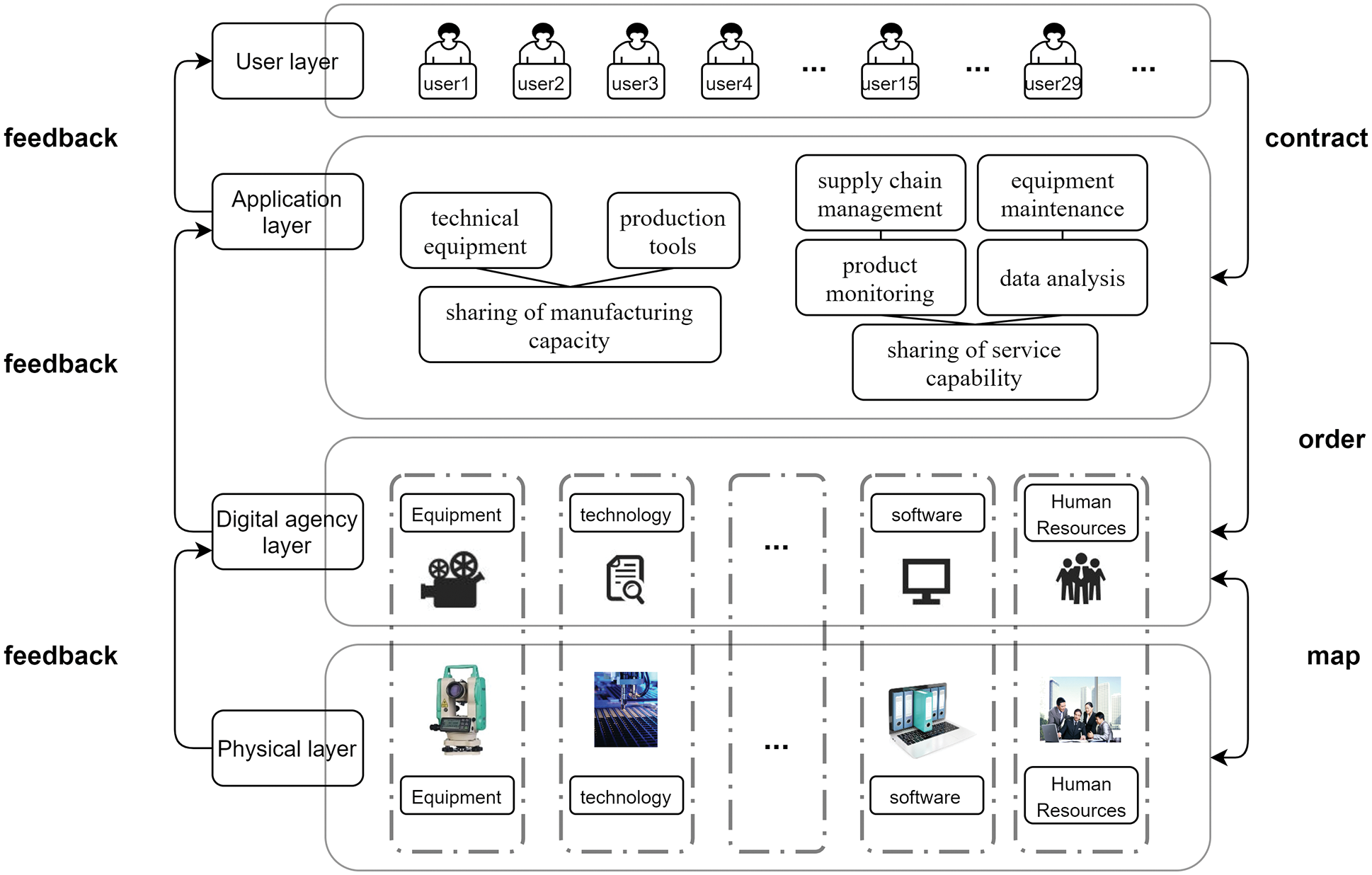
Figure 1: The architecture of shared manufacturing

As a core part of shared manufacturing, shared manufacturing resource allocation is the process of completing manufacturing tasks within a certain amount of time by wise use of restricted resources. Its primary goals are to perform competitive manufacturing resource allocation based on the shared manufacturing entities’ information models, organize manufacturing services for each manufacturing task, and provide a set of services to accommodate personalized manufacturing.

The flexible configuration mode also raises various issues that have not been considered in the conventional configuration mode. In the shared manufacturing environment, the physical resources of different regions and attributes are virtualized into agents. The initial manufacturing environment is more complex, significantly raising the unstable factors. As a result, the most fundamental and crucial area of research for dynamic allocation is the analysis of changes in resource allocation brought on by diverse uncertainty. The resource provider will enter or exit the shared manufacturing according to interest. This paper establishes a model to explore the dynamic allocation of manufacturing tasks and resources in the shared manufacturing process when considering the variation of manufacturing resources.

The rest of the paper will be arranged as follows: Section 2 reviews related work. In Section 3, the model and algorithm of the shared manufacturing resource dynamic allocation problem are proposed. Section 4 presents the numerical example analysis. Finally, the conclusions are given in Section 5.

2  Literature Review

Two streams of the literature are relevant to this section, i.e., the development of shared manufacturing and manufacturing resource allocation.

2.1 Shared Manufacturing

Some fundamental research has been conducted to discuss the concept, the architecture, and the applications of shared manufacturing.

Firstly, the concept of shared manufacturing has been emphasized. Brandt first proposes the concept of shared manufacturing in 1990 [1]. The definition and service operations of shared manufacturing are analyzed in the sharing economy [2]. Yan et al. review supply-demand matching and scheduling in shared manufacturing [3]. Young et al. explore an extension of traditional information-sharing approaches [4]. Under the shared manufacturing mode, Jiang et al. define the concepts associated with three distinct types of shared factories, sharing production-orders, manufacturing-resources, and manufacturing-capabilities [5]. Lujak et al. propose a decentralized coordination approach for multi-robot production planning in openly shared factories [6].

Secondly, it is related to shared manufacturing architecture. He et al. build the basic organizational architecture for the sharing of manufacturing capabilities based on the sharing mode of the shared manufacturing platform [7]. Li et al. propose a brand-new Enhanced Self-organizing Agent in the context of shared manufacturing, which helps the shared manufacturing resources realize cross-sharing with self-organizing communication and negotiation mechanisms [8]. Yu et al. propose the Blockchain-based Shared manufacturing framework [9]. Rozman et al. present an extensible framework for shared manufacturing to establish trust between entities based on blockchain [10]. Zhang et al. establish a reward and punishment mechanism, a subsidy mechanism, and a cost-benefit concept that offer a new framework for improving the quality of shared manufacturing [11]. A hybrid sensing-based approach for monitoring and maintaining shared manufacturing resources is proposed [12]. Wang et al. suggest an integrated architecture to solve the problems of inefficient resource allocation in shared manufacturing as well as help suppliers’ unguaranteed credit [13].

In the third aspect, the application of shared manufacturing is a significant focus of the research. Billo et al. propose a shared manufacturing solution to assess the consolidation and reconfiguration of various industrial operations [14]. Xu et al. investigate online strategy and competitive analysis of production order scheduling problems with the rental cost of shared machines [15]. Xu et al. consider a competitive algorithm for scheduling sharing machines with a rental discount [16]. Li et al. discuss the issue of the equipment manufacturer’s optimal pricing strategy in the selling model and the servitization model [17]. Wei et al. consider two-machine hybrid flow-shop scheduling problems in shared manufacturing [18]. Ji et al. consider parallel-machine scheduling problems in shared manufacturing [19].

2.2 Manufacturing Resource Allocation

The manufacturing resource allocation is to allocate the manufacturing resources of the supplier properly in accordance with its own optimization goal and use the resources as efficiently as possible to accomplish the manufacturing task.

On the one hand, part of the research focuses on the construction of manufacturing resource allocation models. To realize the optimal configuration across various enterprises, Zhang et al. propose an overall architecture for the optimal allocation of manufacturing resources based on community evolution [20]. Yu et al. propose an intelligent-driven green resource allocation mechanism under 5G heterogeneous networks to ensure the high reliability of services [21]. Wu et al. establish a multi-objective integer bi-level multi-follower programming model to simultaneously maximize SoM and QoS from the perspectives of both sides [22]. Lartigau et al. propose a method based on QoS evaluation along with the geo-perspective correlation from one cloud service to another for transportation impact analysis [23]. Tong et al. establish a bi-objective model based on peer effects with an improved grey relational evaluation that aims to maximize satisfaction and minimize individual differences [24]. Aghamohammadzadeh et al. propose a novel platform entitled Blockchain-based service composition model based on Blockchain technology [25].

On the other hand, others try to design and improve the solution method of the manufacturing resource allocation model. Yang et al. present an enhanced multi-objective grey wolf optimizer for the optimal selection problem and multi-objective service composition in cloud manufacturing [26]. Zhang et al. propose an extended flower pollination algorithm to solve the manufacturing service composition problem [27]. Wang et al. develop an evolutionary game model of manufacturing service allocation framework to ensure fairness among users [28]. Que et al. construct a comprehensive mathematical evaluation model with four critical quality of service and awareness indicators, as well as propose a new information entropy immune genetic algorithm for the model’s solution [29]. Li et al. design a Gale–Shapley Algorithm-Based Approach for service composition, which can achieve better performance than the DP method when dealing with a single task or multiple tasks [30]. Gao et al. introduce an improved particle swarm optimization for dynamic service composition. As well, the local greedy algorithm and global reconfiguration method are adopted to restructure composite services dynamically [31].

3  Model and Proposed Approach

3.1 Description of the Dynamic Allocation Problem

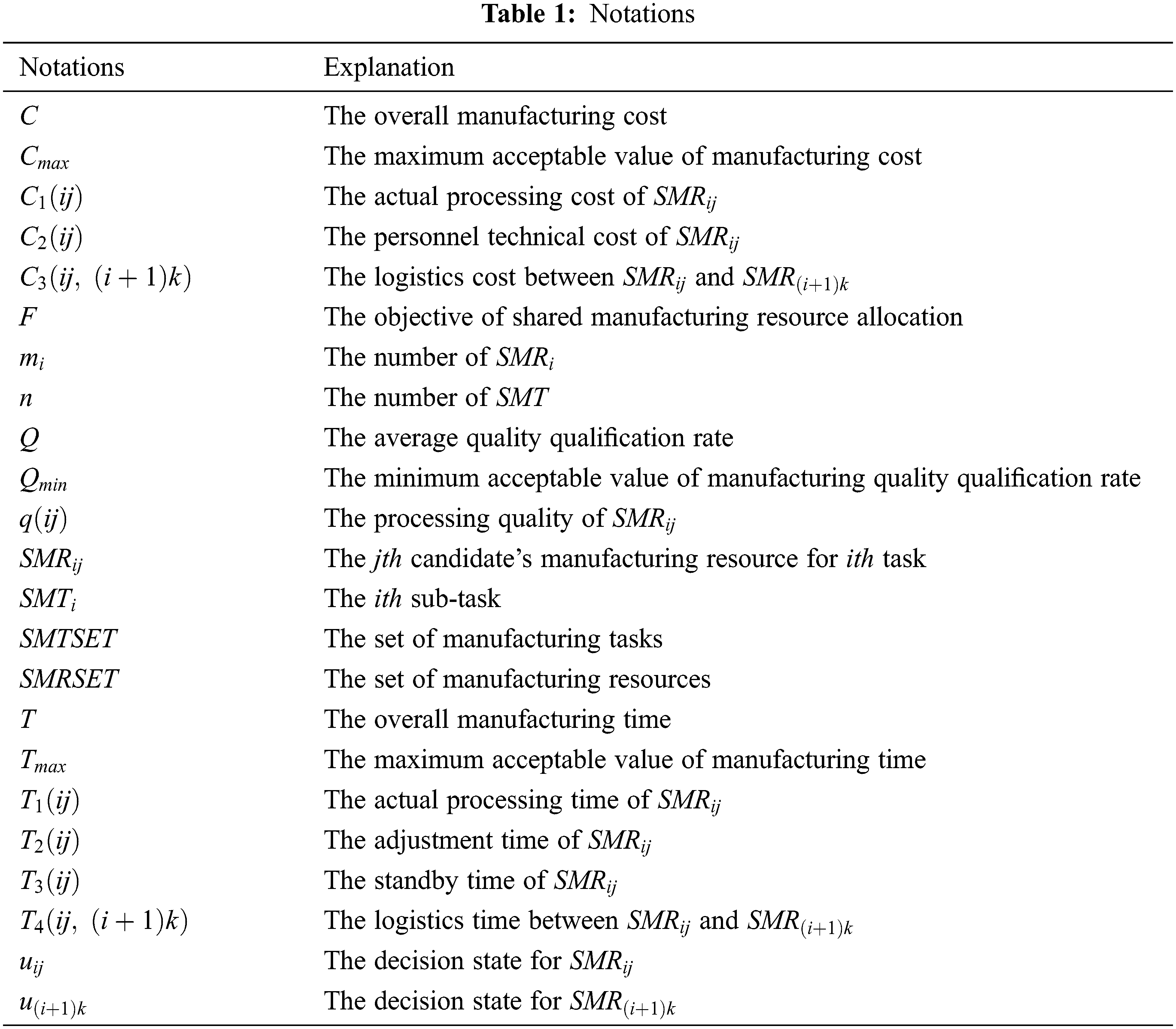
As a dynamic process, shared manufacturing resource allocation is full of changes in the whole process of task execution. The service party offers the use of manufacturing resources and has the right to enter or exit the shared manufacturing process as it sees fit. The demanders provide tasks to be performed and modify or cancel the tasks given out according to their interests. This paper studies how manufacturing resource variation in task execution alters resource allocation. Before beginning a sub-task, the platform provides the optimal configuration of the entire task according to the change in resources. If the manufacturing resources for the candidate remain the same, follow the initial configuration strategy. However, if there is a change in the candidate’s manufacturing resources, they will need to be reconfigured according to the new situation. Therefore, the most significant difference between the manufacturing resource allocation in shared manufacturing and static resource allocation is that the shared manufacturing resource allocation is carried out along with the advancement of sub-tasks, real-time monitoring, and real-time configuration. The primary notations are shown in Table 1.

There are the following provisions:

(1)   One resource can only complete one sub-task.

(2)   One sub-task can only be completed by one resource.

(3)   There is a priority relationship between the sub-tasks, so they need to be completed sequentially.

(4)   Before the sub-task begins, resources can be selected to enter or exit.

(5)   Once the sub-task starts, resources will be locked.

Requirements take the form of a set of tasks and can be denoted as SMTSET={SMTi|i=1, 2, …, n} , where SMTi refers to the ith sub-task. Resources take the form of a set of the candidate’s manufacturing resources. They are marked as SMRSET={SMRij|i=1, 2, …, n; j=1, 2, …, mi} , where the number of the candidate’s manufacturing resources for SMTi is mi , and SMRij represents the jth candidate’s manufacturing resource that can complete the sub-task SMTi .

As an example, consider the case of four sub-tasks. The result of the configuration is 2−1−1−3 before SMT1 starts. SMT1 is performed by SMR12 , SMT2 is performed by SMR21 , SMT3 is performed by SMR31 , and SMT4 is performed by SMR43 . Before the start of SMT2 , the manufacturing resource allocation is 2−2−1 . SMT2 is performed by SMR22 , and the subsequent arrangements are SMR32 for SMT3 and SMR41 for SMT4 . Before SMT3 starts, continue with the current manufacturing resource allocation of 1−2 . SMT3 is performed by SMR31 , and SMT4 is performed by SMR42 . Before SMT4 starts, the configuration result for SMT4 , based on the current candidate’s manufacturing resources, is 1 , and SMT4 is performed by SMR41 , as shown in Fig. 2.

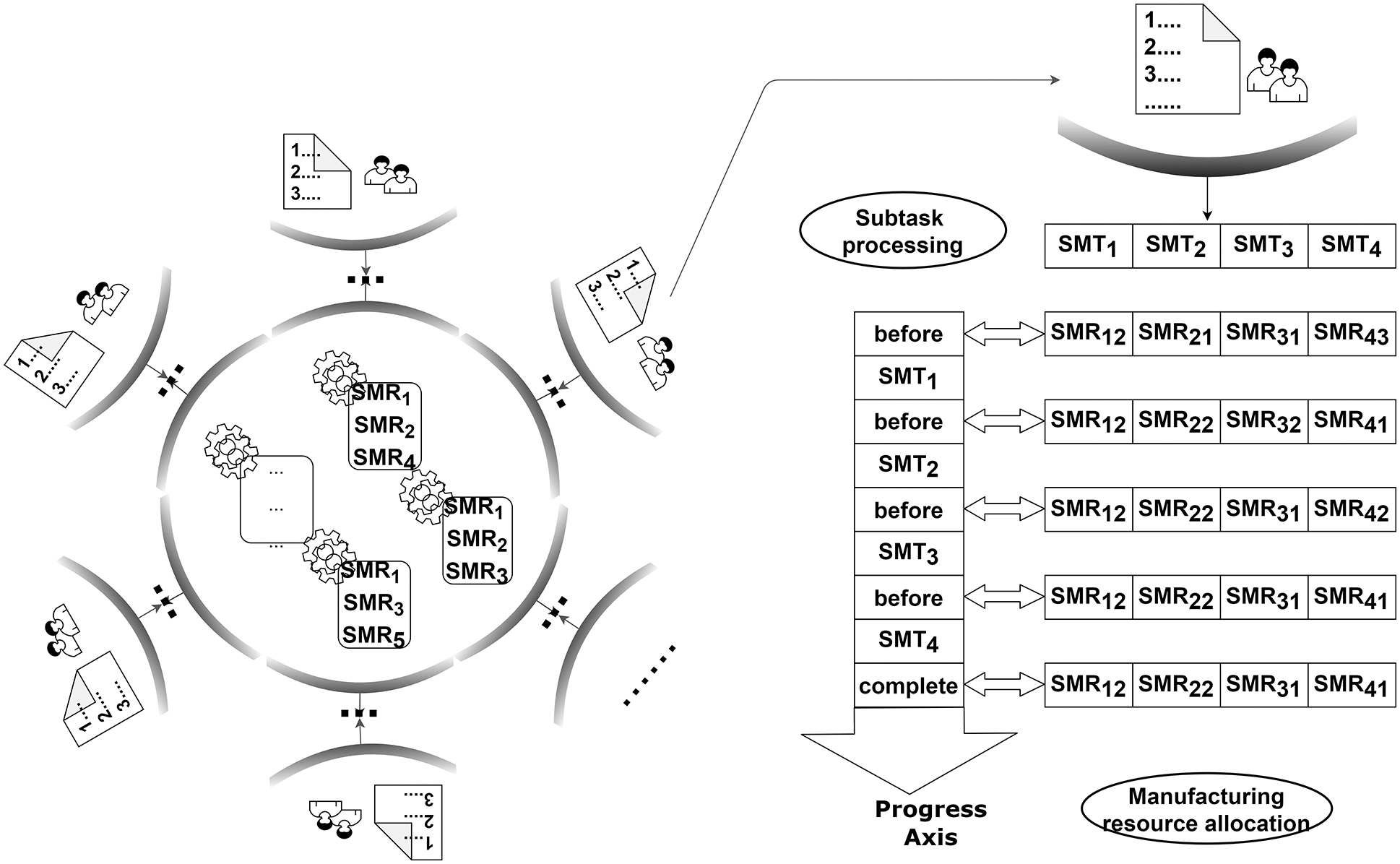
Figure 2: Dynamic allocation of manufacturing resources with sub-task processing

3.2 The Proposed Model

In the whole manufacturing resource allocation, the demanders of manufacturing services, acting as the task’s initiators, give careful consideration to the manufacturing task’s overall quality. The suppliers of manufacturing resources complete the task according to the customized requirements of the demand for manufacturing services. Thus, the demander’s satisfaction directly affects the supplier’s evaluation. Therefore, the service quality indicators become the optimization target of the dynamic allocation model.

The processing cost C is the total of all costs incurred during the production process, from task preparation to completion. The processing cost C is mainly composed of the actual processing cost C1 , the personnel technical cost C2 , and the logistics cost C3 .

Actual processing cost C1 : it is the cost associated with the actual workpieces that were processed using available equipment. The actual processing cost is judged by providers based on historical processing costs and experience, and the specific actual processing cost value is given.

Personnel technical cost C2 : it is the cost of paying related personnel, that is, the cost of human resources for direct or indirect guidance, design, and processing by technicians or experts. The personnel technical cost is evaluated by providers based on the historical processing cost and experience, and a specific personnel technical cost value is provided.

Logistics cost C3 : it is the related cost of the workpieces or materials due to the logistics process. The logistics cost is determined by providers based on the particular geographic location of the workpieces or materials and the historical transportation experience. The specific logistics cost is then given.

Eq. (1) is employed to calculate the processing cost C.

C=∑i=1n[∑j=1miuij(C1(ij)+C2(ij))]+∑i=1n−1[∑j=1mi∑k=1mi+1uiju(i+1)kC3(ij, (i+1)k)] (1)

The processing time T is the total amount of time required for manufacturing tasks, from preparation to completion. Processing time T mainly consists of the actual processing time T1 , the adjustment time T2 , the standby time T3 , and the logistics time T4 .

Actual processing time T1 : it is the amount of time it takes for manufacturing resources to complete actually processing the workpieces. The actual processing time is estimated by providers based on historical processing time and experience.

Adjustment time T2 : it is the time for the unified deployment and debugging of soft resources such as software and human resources for the execution of tasks. The adjustment time is given by providers based on the time of the historic resources call.

Standby time T3 : it refers to the time due to system and path delays when soft resources such as software and labor perform tasks. The standby time is determined by providers based on the completion time of the historical tasks.

Logistics time T4 : it is the logistics time of the actual workpieces or materials. The logistics time is given by providers based on the geographic location and historical experience of the specific sources of the workpieces and materials.

The calculation formula is as Eq. (2).

T=∑i=1n[∑j=1miuij(T1(ij)+T2(ij)+T3(ij))]+∑i=1n−1[∑j=1mi∑k=1mi+1uiju(i+1)kT4(ij, (i+1)k)] (2)

The processing quality Q is the task’s value of processing quality. According to the capability and level of complexity of the workpieces, the quality value of the equipment is given by providers. The calculation formula is Eq. (3).

Q=∑i=1n∑j=1miuijq(ij)n (3)

An optimal allocation model considering shared manufacturing resources is established, taking the lowest processing cost, the shortest processing time, and the most considerable processing quality as the optimization objectives. At the same time, the model must also conform to the constraints of maximum cost, maximum time, and minimum quality, as well as the constraint that only one candidate’s manufacturing resource completes each task, as Eq. (4) shows.

maxF=(CmaxC, TmaxT, QQmin)Ts.t.{C≤CmaxT≤TmaxQ≥Qmin∑j=1miuij=1uij={1, if SMRij is selected0, otherwiseu(i+1)k={1, if SMR(i+1)k is selected0, otherwisei=1, 2, …, n (4)

3.3 Algorithm Design for Shared Manufacturing Resource Allocation Model

The optimal allocation of shared manufacturing resources considering the entries and exits of manufacturing resources is a typical NP-hard problem, so intelligent algorithms are used to solve it. This study will design an NSGA-II and a MOPSO algorithm for the model.

3.3.1 The Operation and Process of the NSGA-II

Given the complexity of the problem of dynamic allocation of shared manufacturing tasks and resources, the chromosomal coding rules for this paper are as follows: SMTi means the ith sub-task, and SMRij means the jth candidate’s manufacturing resource for the ith task. The coding rules are shown in Fig. 3.

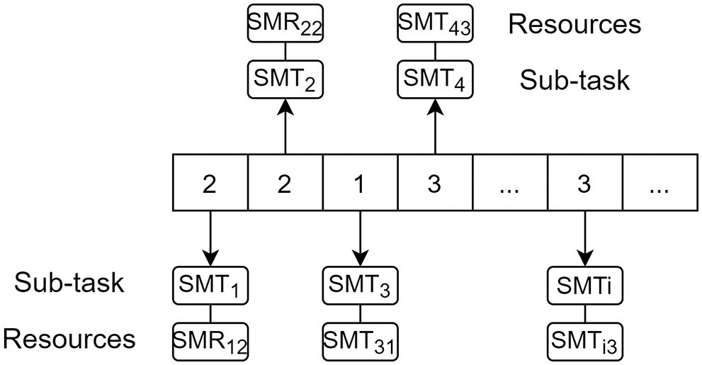
Figure 3: Rules for chromosome coding

We adjust the matrix Q from the first bit. If the value of the gene encoding i in the matrix K is K[1, i] , the value of the K[1, i]th row and the ith column in the matrix Q will be 1. This process is applied repeatedly and sequentially to each bit in the matrix K. Eventually, the matrix Q is the result of decoding, that is, the result of manufacturing resource allocation. For example, K=[2312] decodes as Q=[001010010100] .

The process of the NSGA-II is shown in Fig. 4.

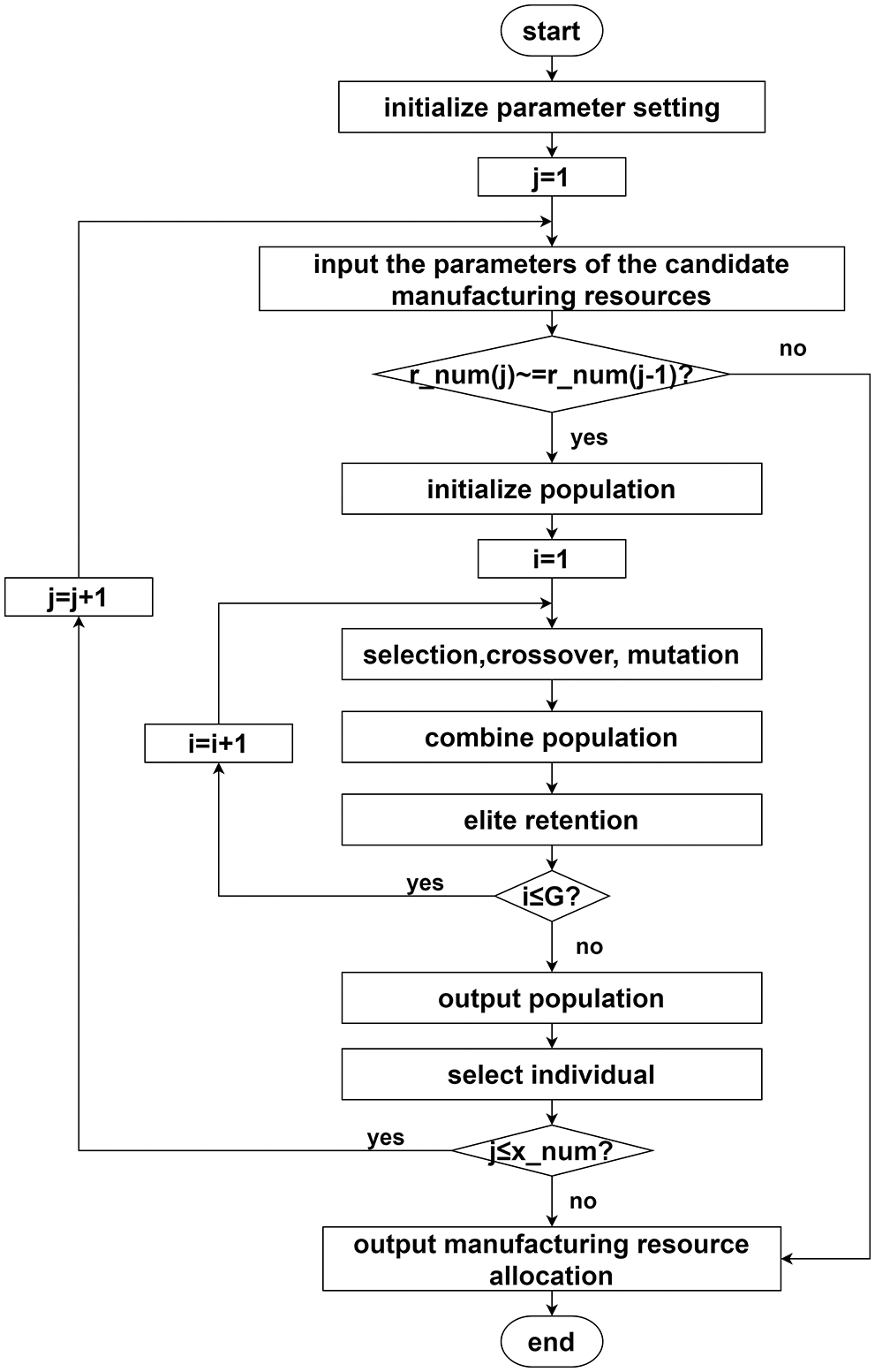
Figure 4: The process of the NSGA-II

The NSGA-II is implemented as follows:

Step 1: Set the parameters. The population size is set to NP , the maximum iteration number is G, the crossover probability is pc , the mutation probability is pm , the fitness function number is f_num , the number of tasks is x_num , and the number of the initial candidate’s manufacturing resources is r_num(0) . The maximum cost is Cmax , the longest time is Tmax , and the minimum qualified rate is Qmin .

Step 2: Input the parameters of the candidate’s manufacturing resources. Each task corresponds to actual processing cost C1 , personnel technical cost C2 , logistics cost C3 , actual processing time T1 , adjustment time T2 , standby time T3 , logistics time T4 , and processing quality Q of the candidate’s manufacturing resources.

Step 3: Judge whether r_num(j) has changed compared with r_num(j−1) before starting the sub-task. If yes, continue to the next step; if not, skip to Step 12.

Step 4: Initialize the population and generate the parent population.

The initial population is randomly generated. The number σ between 0 and 1 is random, and the initial parent population X1t is obtained according to Eq. (5).

X1t=[(x_min+(x_max−x_min)∗σ)] (5)

Step 5: Selection, crossover, and mutation operations are carried out to produce the offspring population.

Non-uniform arithmetic crossover is used. v is randomly generated with iterations, and η is determined according to Eq. (6). Then, the crossover individuals X1t+1 and X2t+1 are determined according to Eq. (7).

η={(2v)1a+1, v<0.5[12(1−v)]1a+1, v≥0.5 (6)

{X1t+1=⌈0.5[(1+η)X1t+(1−η)X2t]⌉X2t+1=⌈0.5[(1−η)X1t+(1+η)X2t]⌉ (7)

The non-uniform mutation is used. The parameter u is randomly generated, and ζ is determined by Eq. (8). Then Eq. (9) is employed to get the offspring individual X1t+1 .

ζ={(2u)1b+1−1, u<0.51−[2(1−u)]1b+1, u≥0.5 (8)

X1t+1=⌈X1t+ζ⌉ (9)

Step 6: Combine the parent population with the offspring population.

Step 7: Elite retention.

Step 8: Judge whether the number of iterations i is less than or equal to G. If yes, jump to Step 5; if no, continue to the next step.

Step 9: Output population.

Step 10: Select individuals in the Pareto frontier as the resource allocation plan for subsequent processing.

Step 11: Judge whether j is less than x_num . If yes, jump to Step 2; if no, continue to the next step.

Step 12: Output the result of manufacturing resource allocation.

3.3.2 The Operation and Process of the MOPSO Algorithm

The optimal allocation is obtained by updating the velocity of particles, the position of particles, and the inertia weight in the MOPSO algorithm. Among them, velocity represents the speed of movement, and position represents the direction of movement.

The process of the MOPSO algorithm is shown in Fig. 5.

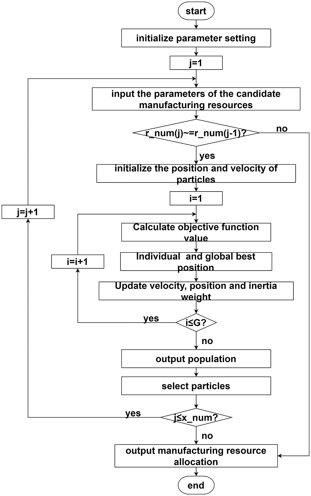
Figure 5: The process of the MOPSO algorithm

The MOPSO algorithm is implemented as follows:

Step 1: Set the parameters. The population size is set to nPop , the maximum iteration number is MaxIt , the number of tasks is nVar , the number of the initial candidate’s manufacturing resources is r_num(0) , the personal learning coefficient is c1 , the global learning coefficient is c2 , the inertia weight is w, and the inertia weight damping ratio is wdamp . The maximum cost is Cmax , the longest time is Tmax , and the minimum qualified rate is Qmin .

Step 2: Input the parameters of the candidate’s manufacturing resources. Each task corresponds to actual processing cost C1 , personnel technical cost C2 , logistics cost C3 , actual processing time T1 , adjustment time T2 , standby time T3 , logistics time T4 , and processing quality Q of the candidate’s manufacturing resources.

Step 3: Judge whether r_num(j) has changed compared with r_num(j−1) before starting the sub-task. If yes, continue to the next step; if not, skip to Step 12.

Step 4: Initialize the position and velocity of particles.

The position and velocity of particles are randomly selected in order to generate the initial population.

Step 5: Calculate the objective functions to find the optimum fitness value.

Step 6: Find the individual’s best position and global best position.

Step 7: Update velocity, position, and inertia weight.

Eq. (10) is employed to update the velocity of particles Vij(t+1) , Eq. (11) is employed to update the position of particles Yij(t+1) , and the inertia weight w is determined according to Eq. (12).

Vij(t+1)=wVij(t)+c1r1(t)[Pij(t)−Yij(t)]+c2r2(t)[Pgj(t)−Yij(t)] (10)

Yij(t+1)=Yij(t)+Vij(t+1) (11)

w=w⋅wdamp (12)

Step 8: Judge whether the number of iterations i is less than or equal to MaxIt . If yes, jump to Step 5; if no, continue to the next step.

Step 9: Output population.

Step 10: Select particles in the Pareto frontier as the resource allocation plan for subsequent processing.

Step 11: Judge whether j is less than nVar . If yes, jump to Step 2; if no, continue to the next step.

Step 12: Output the result of manufacturing resource allocation.

4  Numerical Example Analysis

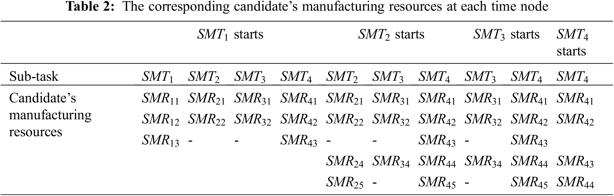
There are four sub-tasks. The sub-task SMT1 can be performed by three candidate’s manufacturing resources ( SMR11 , SMR12 , and SMR13 ), SMT2 is performed by two candidate’s manufacturing resources ( SMR21 and SMR22 ), SMT3 is performed by two candidate’s resources ( SMR31 and SMR32 ), and SMT4 is performed by three candidate’s manufacturing resources ( SMR41 , SMR42 , and SMR43 ). Then, following the completion of the sub-task SMT1 , it is found that the candidate’s manufacturing resources have changed. That is, SMR24 , SMR25 , SMR34 , SMR44 and SMR45 enter the candidate’s manufacturing resource set. Among them, SMT2 can be performed by SMR24 and SMR25 , SMT3 can be performed by SMR34 , and SMT4 can be performed by SMR44 and SMR45 . Later, after SMT2 is completed, the corresponding candidate’s manufacturing resources for each sub-task have not changed. Finally, after the sub-task SMT3 is completed, SMR45 exits, so the set of candidates’ manufacturing resources changes again.

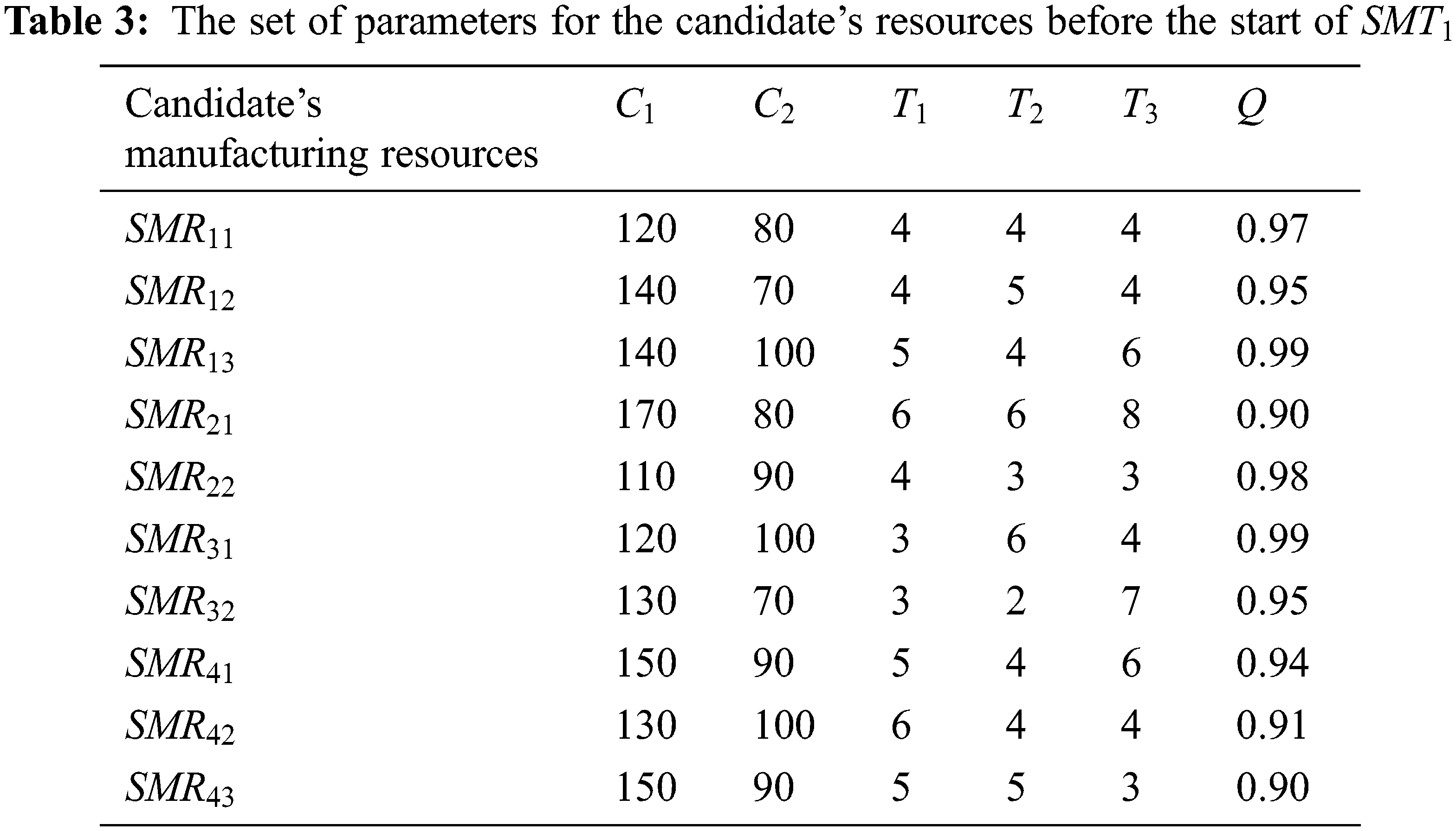
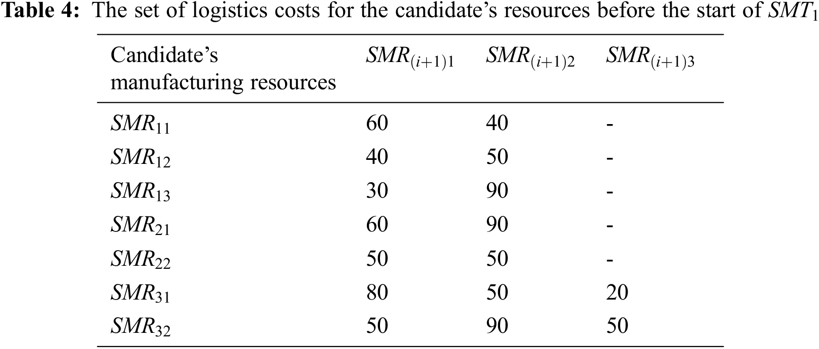
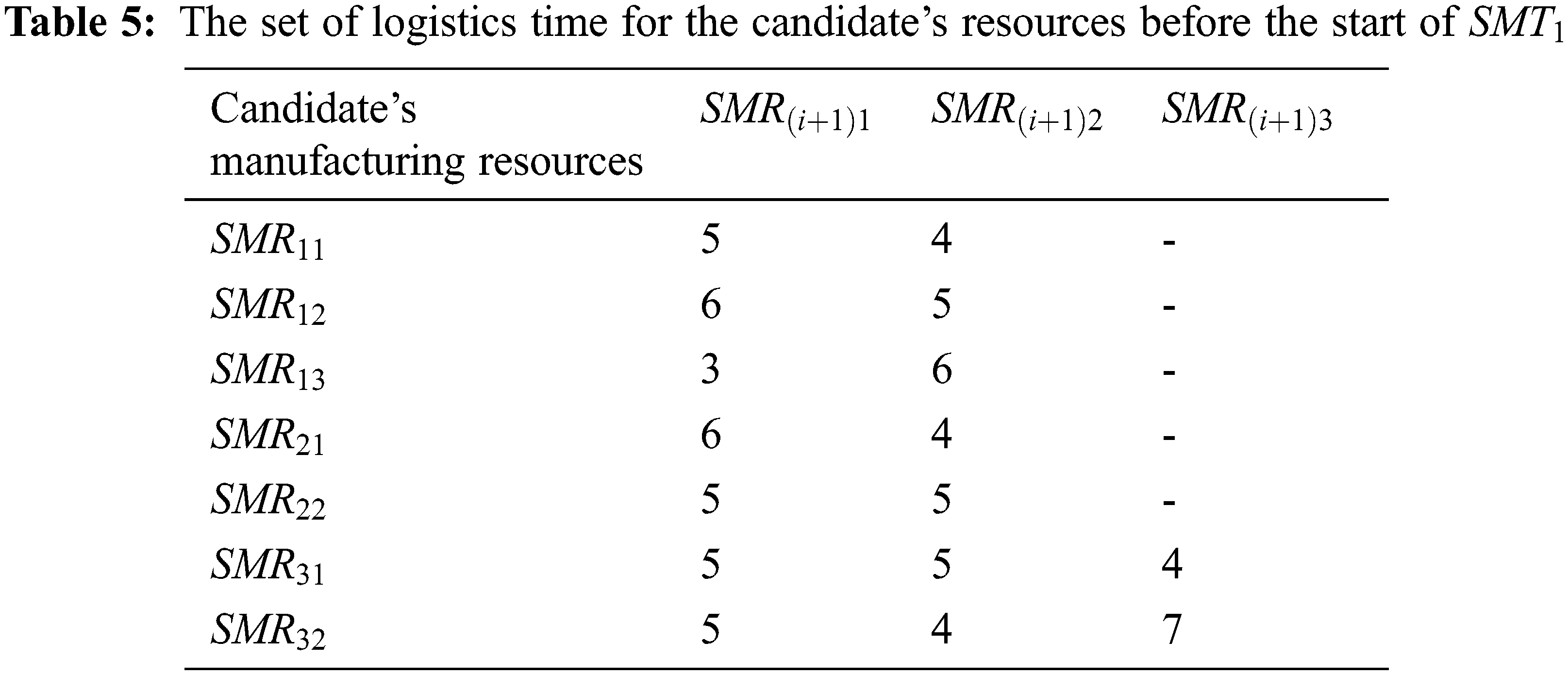
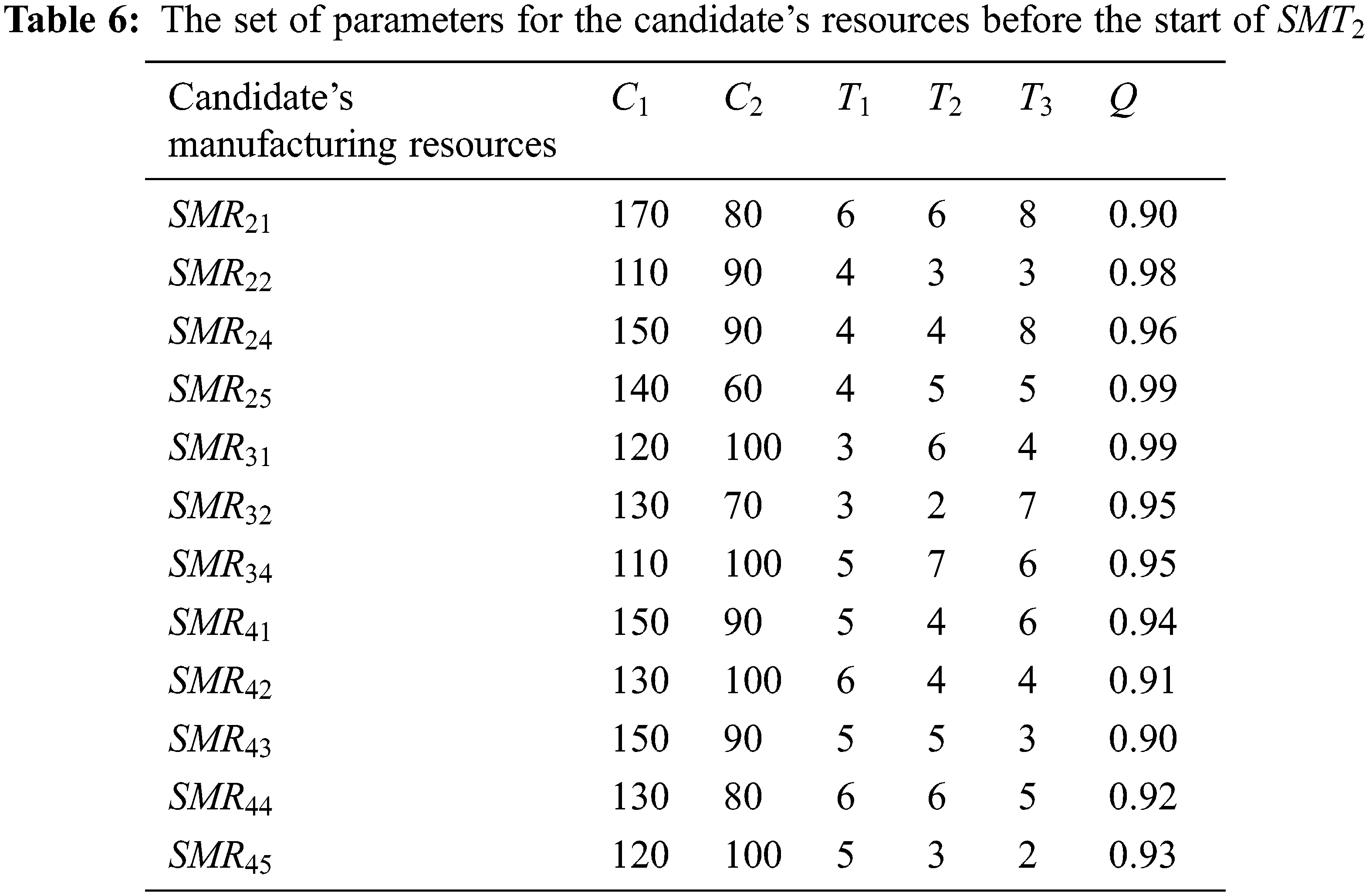
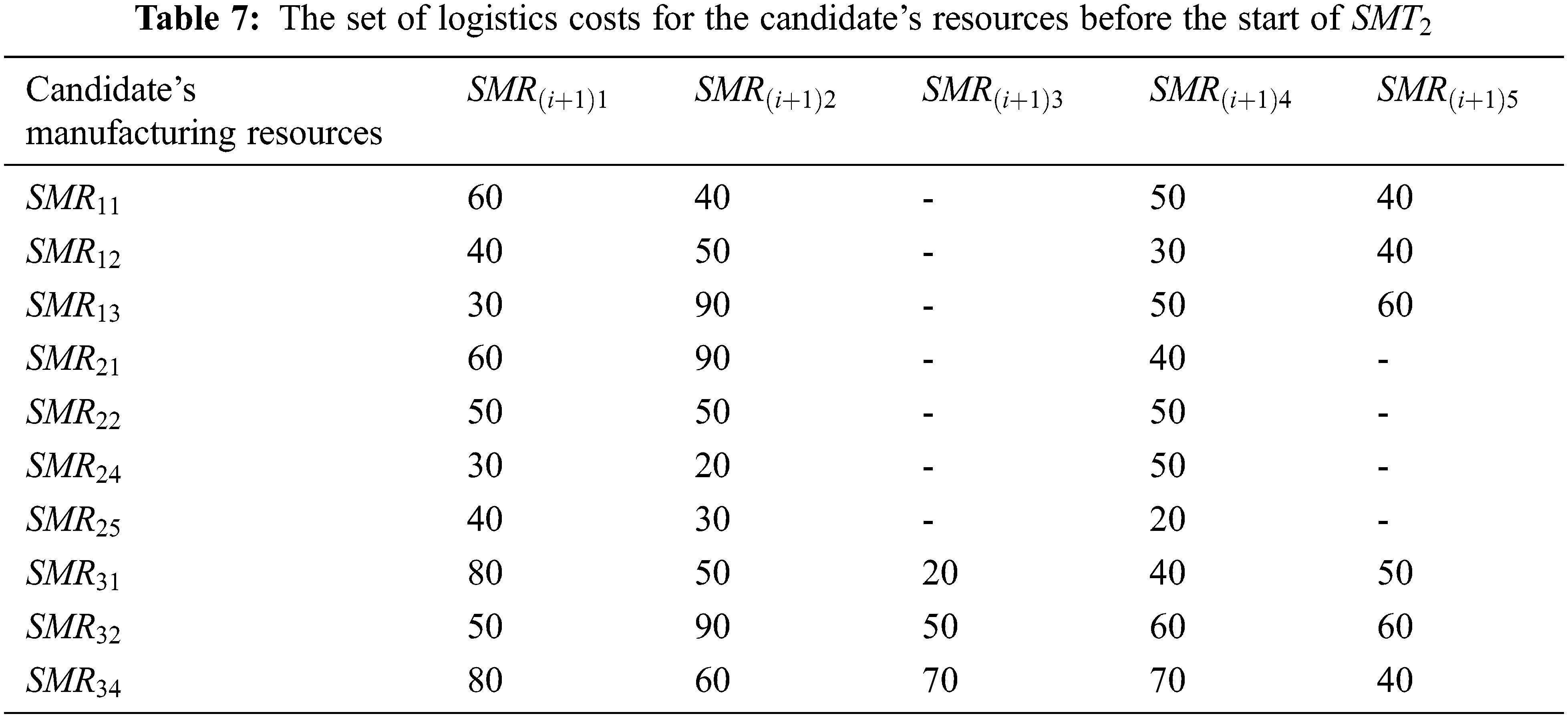
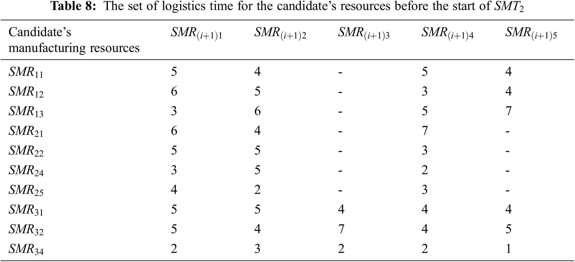
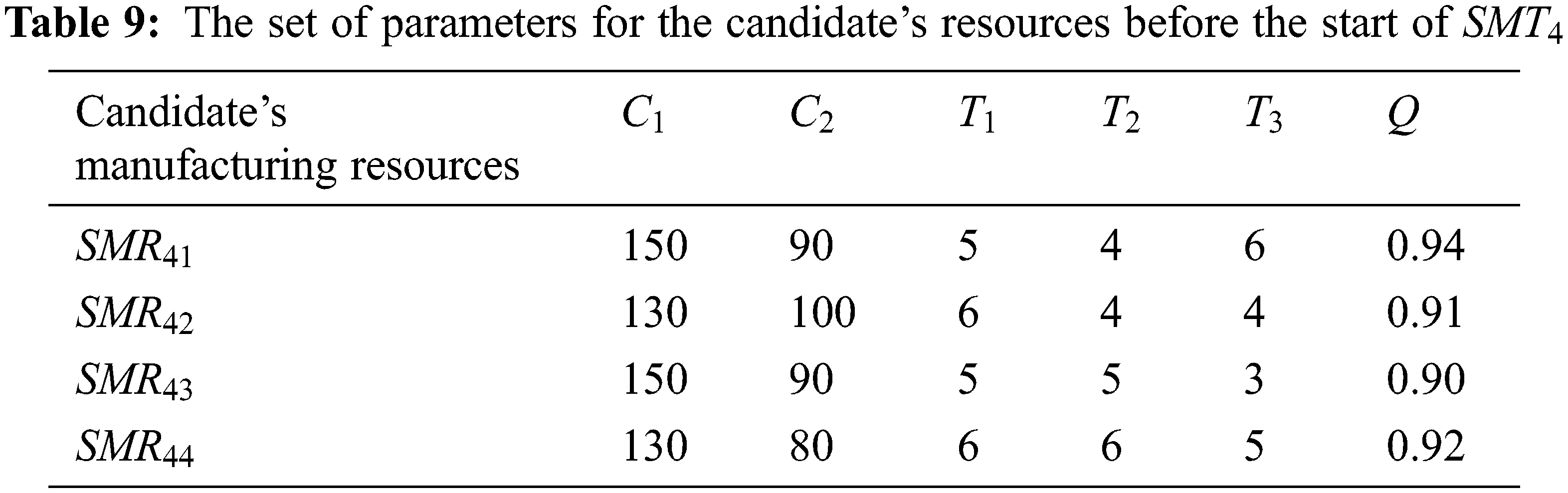
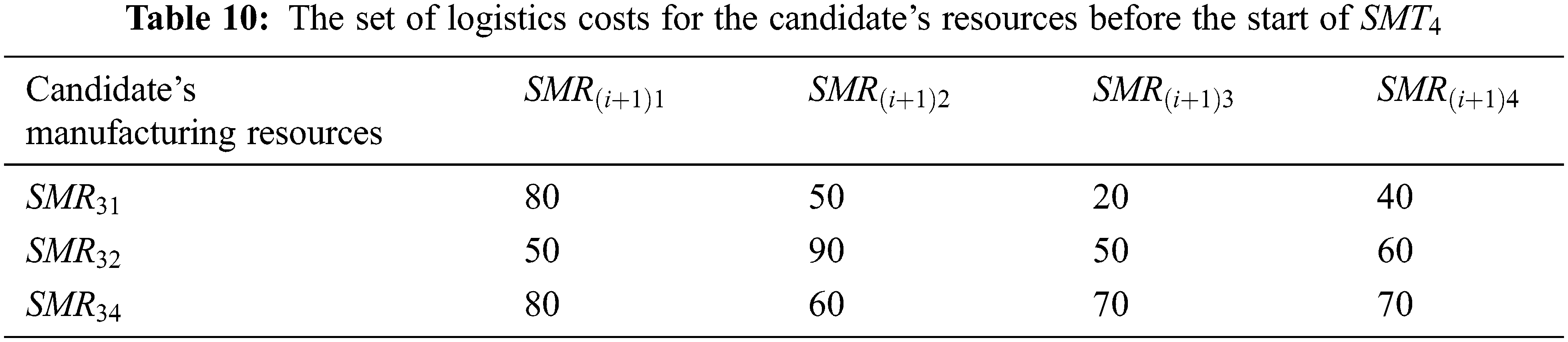
The candidate’s manufacturing resources corresponding to the manufacturing sub-tasks at each time node are shown in Table 2. The related parameters of each candidate’s manufacturing resource before the start of the sub-task SMT1 are shown in Tables 3–5. In Tables 6–8, these are the parameters before the beginning of SMT2 . In addition, the parameters before the beginning of the sub-task SMT4 are shown in Tables 9–11. Furthermore, Cmax is 1100, Tmax is 90, and Qmin is 0.6.

The NSGA-II and MOPSO algorithms are coded with MATLAB (R2018a), and all numerical experiments are performed on a computer with Intel (R) Core (TM) i5-1155G7 @2.50 GHz CPU and 16.0 GB RAM under Window 11 Home 64-bit operating environment.

4.1 The Parameters in the NSGA-II and MOPSO Algorithms

Based on the resource allocation performed before the start of SMT1 , the operating results of the NSGA-II and MOPSO algorithms are analyzed.

In NSGA-II, when the iteration number is 110, the average values of resource allocation of SMT1 with different population sizes are calculated, and the evolutions are shown in Fig. 6. Obviously, the average values of fitness remain stable after the population size reaches 120. Similarly, when the population size is 120, the average values of fitness of SMT1 running 10 times under different iterations are calculated, and the evolutions are shown in Fig. 7. Obviously, the average values of fitness remain stable after the iteration number reaches 110.

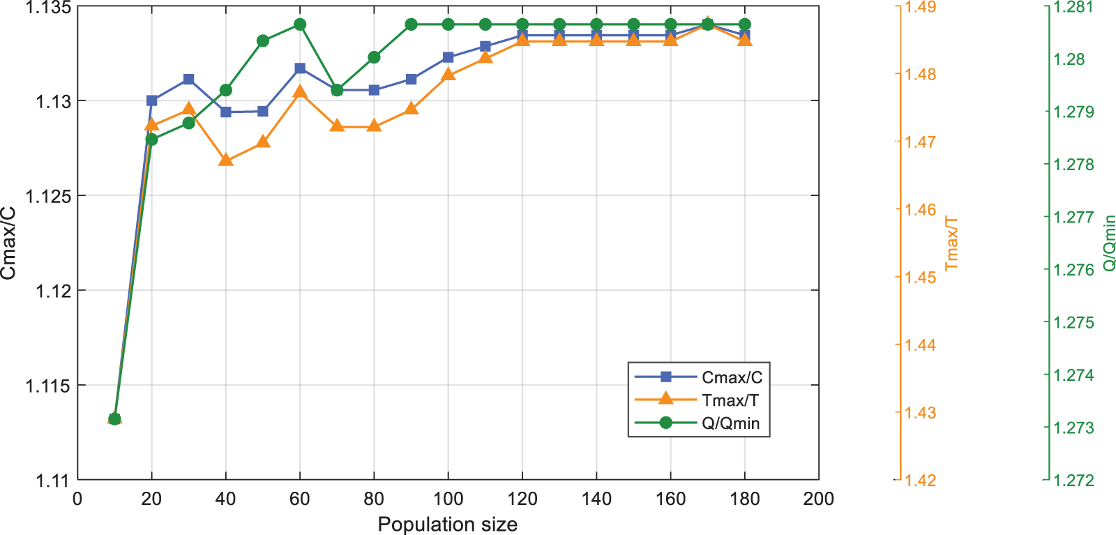
Figure 6: The average values of fitness when the iteration number is 110 in the NSGA-II

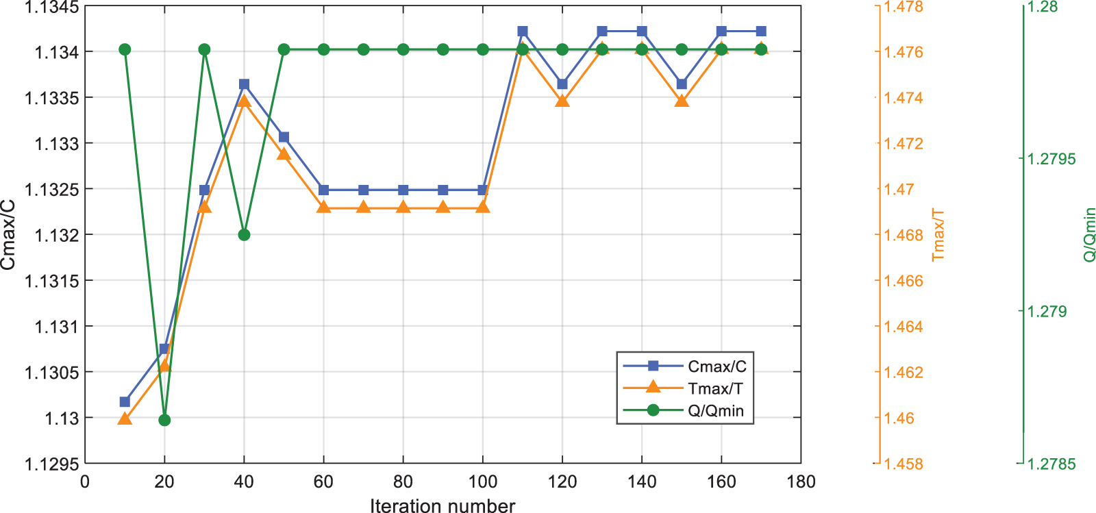
Figure 7: The average values of fitness when the population size is 120 in the NSGA-II

In MOPSO algorithm, when the iteration number is 30, the average values of resource allocation of SMT1 with different population sizes are calculated, and the evolutions are shown in Fig. 8. Obviously, the average values of fitness remain stable after the population size reaches 70. Similarly, when the population size is 70, the average values of fitness of SMT1 running 10 times under different iterations are calculated, and the evolutions are shown in Fig. 9. Obviously, the average values of fitness remain stable after the iteration number reaches 30.

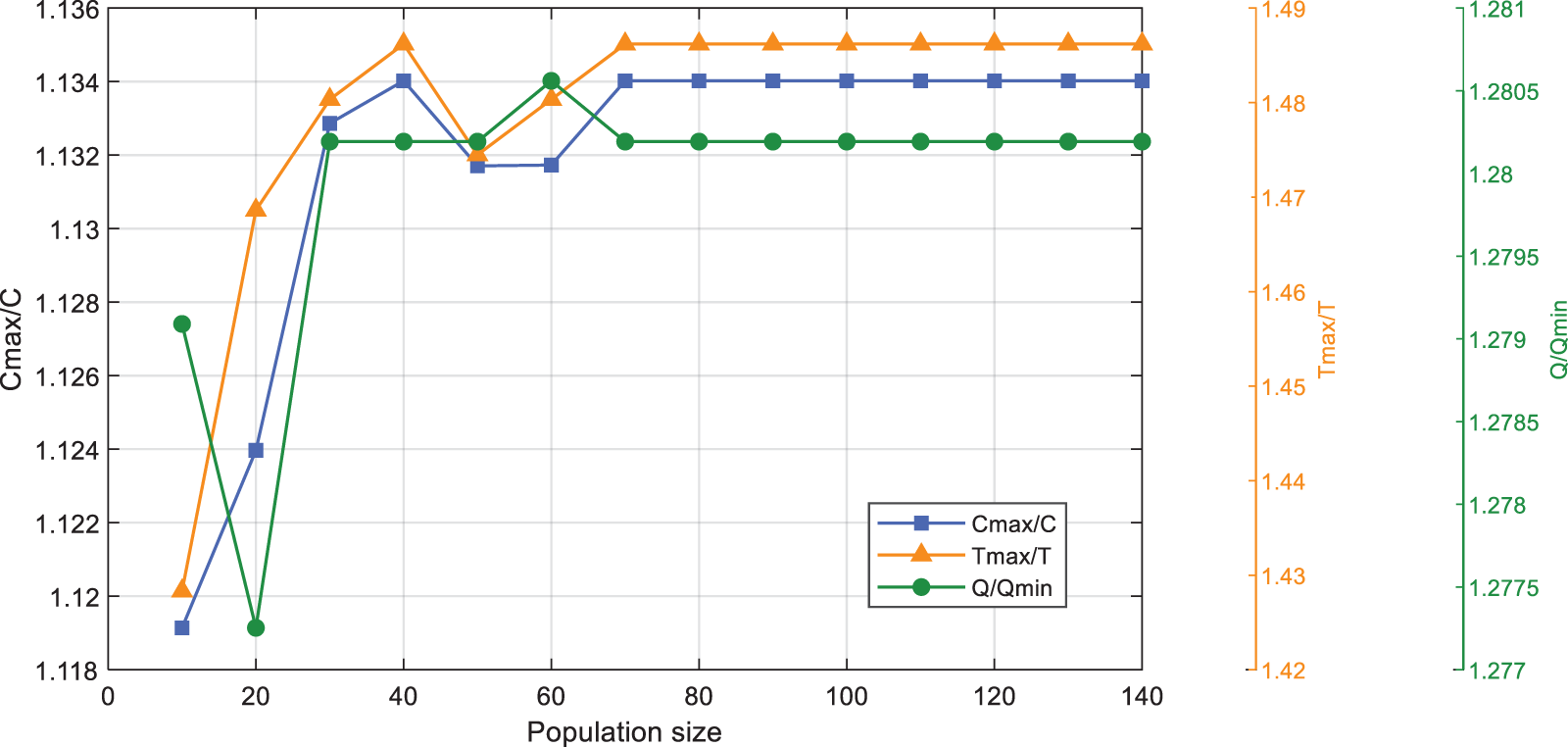
Figure 8: The average values of fitness when the iteration number is 30 in the MOPSO algorithm

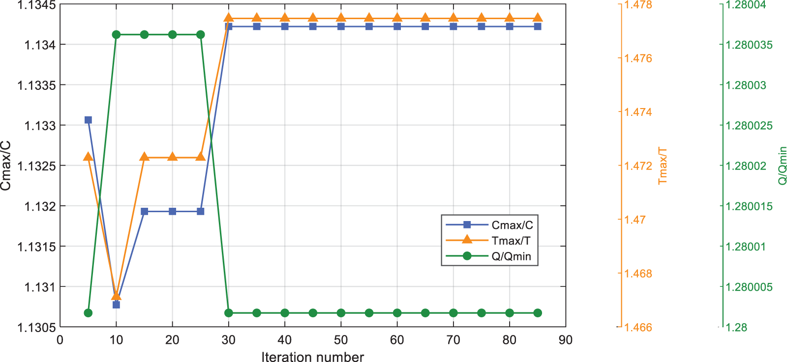
Figure 9: The average values of fitness when the population size is 70 in the MOPSO algorithm

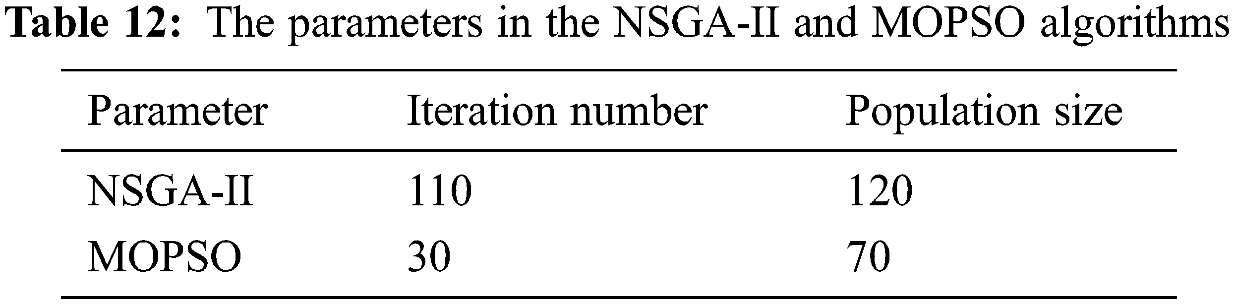
According to the above experiments, the optimal settings of parameters for operation in the NSGA-II and MOPSO algorithms have been obtained. Therefore, the population size in the NSGA-II is set to 120, and the population size in the MOPSO algorithm is set to 70. The parameters in the NSGA-II and MOPSO algorithms are listed in Table 12.

4.2 The Results of Dynamic Resource Allocation

The model’s resource allocation for each sub-tasks is obtained, as shown in Table 13.

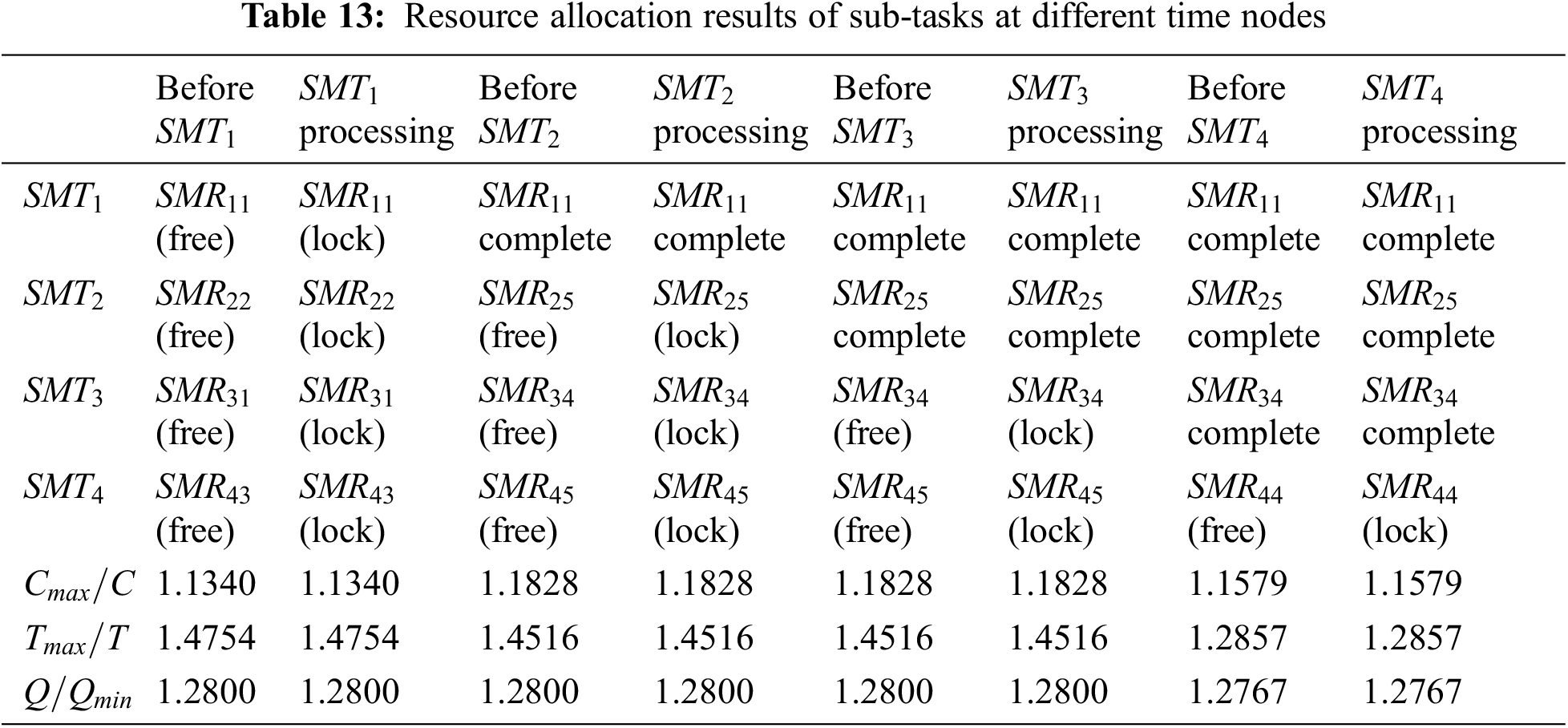
Before SMT1 starts, shared manufacturing resource allocation is that sub-task SMT1 is performed by resource SMR11 , SMT2 is performed by SMR22 , SMT3 is performed by SMR31 , and SMT4 is performed by SMR43 . During SMT1 processing, the configured resources SMR11 , SMR22 , SMR31 , and SMR43 will be locked. After SMT1 is completed, SMR22 , SMR31 , and SMR43 are unlocked and free.

Before SMT2 starts, new resources are found to enter based on the monitoring of the candidate’s manufacturing resources, so shared manufacturing resources need to be reconfigured. At this point, SMT2 is performed by SMR25 , SMT3 is performed by SMR34 , and SMT4 is performed by SMR45 . During SMT2 processing, configured resources SMR25 , SMR34 , and SMR45 will be locked. After SMT2 is completed, SMR34 and SMR45 are unlocked and free.

Before SMT3 starts, no change in the candidate’s manufacturing resources is detected, so the allocation is maintained. That is, SMT3 is performed by SMR34 , and SMT4 is performed by SMR45 . The configured resources SMR34 and SMR45 will be locked during SMT3 processing. After SMT3 is completed, SMR45 is unlocked and free.

Before SMT4 starts, some of the candidate’s manufacturing resources are detected to exit, so the resources are reconfigured, and SMT4 is performed by SMR44 .

Finally, with the progress of the sub-tasks, the dynamic manufacturing resource allocation is completed.

4.3 Analysis of Operating Results

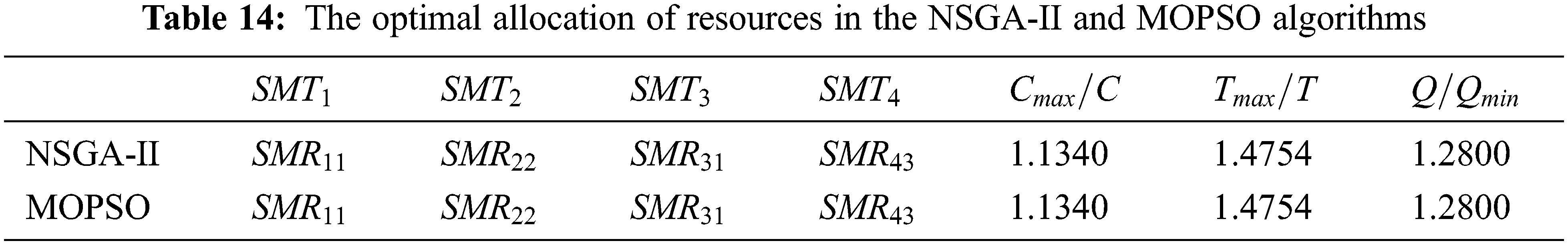
The optimal resource allocation obtained by running two algorithms overlaps, as shown in Table 14, proves the effectiveness of the model.

Through repeated experiments, it is found that the NSGA-II can generate more stable populations than the MOPSO algorithm. Figs. 10 and 11 are three-dimensional graphs of the results of multiple runs under the NSGA-II and MOPSO algorithms. On the other hand, the evolution of the running time in two algorithms with different iteration numbers is shown in Fig. 12. When the iteration count of the two algorithms is less than 20, there is not much of a difference in the running times—both take about 5 s. However, with an increase in iteration numbers, the MOPSO algorithm operates much more rapidly than the NSGA-II.

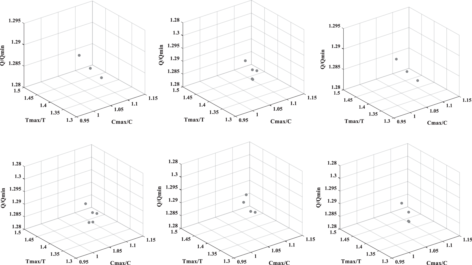
Figure 10: The running results of the NSGA-II

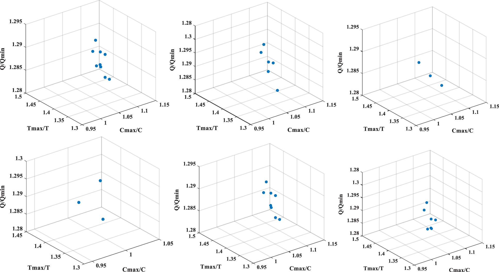
Figure 11: The running results of the MOPSO algorithm

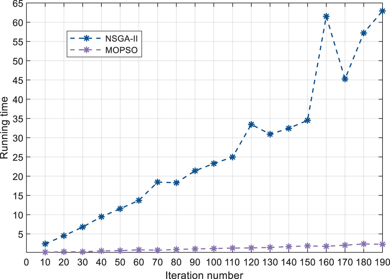
Figure 12: The running time of the NSGA-II and MOPSO varies with the iteration number

5  Conclusions and Future Work

This paper describes the dynamic allocation in the shared manufacturing environment. Furthermore, a model considering the entries or exits of the candidate’s manufacturing resources at various time nodes is put forth. Then, the NSGA-II and MOPSO algorithms are designed to solve the model. Furthermore, the two algorithms are compared and analyzed with a numerical example, and the efficiency of the model is proved. Finally, the conclusions are drawn, and future work is analyzed.

The main contributions of this paper can be summarized as follows. Firstly, we describe the problem of optimal allocation of manufacturing resources in shared manufacturing and the characteristics of shared manufacturing resource allocation. Secondly, a dynamic allocation model of manufacturing tasks and resources is proposed. Thirdly, the NSGA-II and MOPSO algorithms are designed to solve the resource allocation model with the processing of tasks. Finally, by comparing and analyzing the running results of the two algorithms through a numerical example, the effectiveness of the manufacturing resource allocation model, considering the variation of resources, is confirmed.

The future work may include several aspects: (1) Allocation of shared manufacturing resources in accordance with task variation. Task demand is another critical destabilizing factor in shared manufacturing, and its variation will inevitably lead to changes in how manufacturing resources are allocated. (2) Improvements to existing algorithms. Given the slow running speed of the NSGA-II and the unstable MOPSO algorithm, a method with a faster running speed and a more accurate result will be analyzed and discussed.

Acknowledgement: The authors wish to acknowledge the contribution of Liaoning Key Lab of Equipment Manufacturing Engineering Management, Liaoning Research Base of Equipment Manufacturing Development, Liaoning Key Research Base of Humanities and Social Sciences: Research Center of Micro-management Theory of SUT.

Funding Statement: This work was supported by the Key Program of Social Science Planning Foundation of Liaoning Province under Grant L21AGL017.

Conflicts of Interest: The authors declare that they have no conflicts of interest to report regarding the present study.

References

1. E. Brandt, “A vision for shared manufacturing,” Mechanical Engineering, vol. 112, pp. 52–55, 1990. [Google Scholar]
2. C. Y. Yu, X. Xu, S. Q. Yu, Z. Q. Sang, C. Yang et al., “Shared manufacturing in the sharing economy: Concept, definition and service operations,” Computers & Industrial Engineering, vol. 146, pp. 106602, 2020. [Google Scholar]
3. P. Y. Yan, L. Yang and A. Che, “Review of supply-demand matching and scheduling in shared manufacturing,” Systems Engineering-Theory & Practice, vol. 42, no. 3, pp. 811–832, 2022. [Google Scholar]
4. B. Young, A. F. Cutting-Decelle, D. Guerra, G. Gunendran, B. Das et al., “Sharing manufacturing information and knowledge in design decision and support,” in Proc. of 5th Int. Conf. on Integrated Design and Manufacturing in Mechanical Engineering, Univ Bath, Bath, England, pp. 173–185, 2005. [Google Scholar]
5. P. Y. Jiang and P. L. Li, “Shared factory: A new production node for social manufacturing in the context of sharing economy,” Proceedings of the Institution of Mechanical Engineers. Part B: Journal of Engineering Manufacture, vol. 234, no. 1–2, pp. 285–294, 2020. [Google Scholar]
6. M. Lujak, A. Fernandez and E. Onaindia, “Spillover algorithm: A decentralised coordination approach for multi-robot production planning in open shared factories,” Robotics and Computer-Integrated Manufacturing, vol. 70, pp. 102110, 2021. [Google Scholar]
7. J. B. He, J. Zhang and X. J. Gu, “Research on sharing manufacturing in Chinese manufacturing industry,” International Journal of Advanced Manufacturing Technology, vol. 104, no. 1–4, pp. 463–476, 2019. [Google Scholar]
8. P. L. Li and P. Y. Jiang, “Enhanced agents in shared factory: Enabling high-efficiency self-organization and sustainability of the shared manufacturing resources,” Journal of Cleaner Production, vol. 292, pp. 126020, 2021. [Google Scholar]
9. C. Yu, X. Jiang, S. Yu and C. Yang, “Blockchain-based shared manufacturing in support of cyber physical systems: Concept, framework, and operation,” Robotics and Computer-Integrated Manufacturing, vol. 64, pp. 101931, 2020. [Google Scholar]
10. N. Rozman, J. Diaci and M. Corn, “Scalable framework for blockchain-based shared manufacturing,” Robotics and Computer-Integrated Manufacturing, vol. 71, pp. 102139, 2021. [Google Scholar]
11. Z. Zhang, X. Wang, C. Su and L. Sun, “Evolutionary game analysis of shared manufacturing quality synergy under dynamic reward and punishment mechanism,” Applied Sciences, vol. 12, no. 13, pp. 6792, 2022. https://doi.org/10.3390/app12136792 [Google Scholar] [CrossRef]
12. G. Zhang, C. H. Chen, B. F. Liu, X. Y. Li and Z. X. Wang, “Hybrid sensing-based approach for the monitoring and maintenance of shared manufacturing resources,” International Journal of Production Research, 2021. https://doi.org/10.1080/00207543.2021.2013564 [Google Scholar] [CrossRef]
13. G. Wang, G. Zhang, X. Guo and Y. Zhang, “Digital twin-driven service model and optimal allocation of manufacturing resources in shared manufacturing,” Journal of Manufacturing Systems, vol. 59, pp. 165–179, 2021. [Google Scholar]
14. R. E. Billo, F. Dearborn, C. J. Hostick, G. E. Spanner, E. J. Stahlman et al., “A group technology model to assess consolidation and reconfiguration of multiple industrial operations—A shared manufacturing solution,” International Journal of Computer Integrated Manufacturing, vol. 6, no. 5, pp. 311–322, 1993. [Google Scholar]
15. Y. F. Xu, R. T. Zhi, F. F. Zheng and M. Liu, “Online strategy and competitive analysis of production order scheduling problem with rental cost of shared machines,” Chinese Journal of Management Science, 2021. https://doi.org/10.16381/j.cnki.issn1003-207x.2020.1663 [Google Scholar] [CrossRef]
16. Y. Xu, R. Zhi, F. Zheng and M. Liu, “Competitive algorithm for scheduling of sharing machines with rental discount,” Journal of Combinatorial Optimization, vol. 44, no. 1, pp. 414–434, 2022. [Google Scholar]
17. K. Li, W. Xiao and X. X. Zhu, “Pricing strategies for sharing manufacturing model based on the cloud platform,” Control and Decision, vol. 37, no. 4, pp. 1056–1066, 2022. [Google Scholar]
18. Q. Wei and Y. Wu, “Two-machine hybrid flow-shop problems in shared manufacturing,” Computer Modeling in Engineering & Sciences, vol. 131, no. 2, pp. 1125–1146, 2022. [Google Scholar]
19. M. Ji, X. N. Ye, F. Y. Qian, T. C. E. Cheng and Y. W. Jiang, “Parallel-machine scheduling in shared manufacturing,” Journal of Industrial and Management Optimization, vol. 18, no. 1, pp. 681–691, 2022. [Google Scholar]
20. Y. F. Zhang, D. Zhang, Z. Wang and C. Qian, “An optimal configuration method of multi-level manufacturing resources based on community evolution for social manufacturing,” Robotics and Computer-Integrated Manufacturing, vol. 65, pp. 101964, 2020. [Google Scholar]
21. P. Yu, M. Yang, A. Xiong, Y. H. Ding, W. J. Li et al., “Intelligent-driven green resource allocation for industrial internet of things in 5G heterogeneous networks,” IEEE Transactions on Industrial Informatics, vol. 18, no. 1, pp. 520–530, 2022. [Google Scholar]
22. Y. X. Wu, G. Z. Jia and Y. Cheng, “Cloud manufacturing service composition and optimal selection with sustainability considerations: A multi-objective integer bi-level multi-follower programming approach,” International Journal of Production Research, vol. 58, no. 19, pp. 6024–6042, 2020. [Google Scholar]
23. J. Lartigau, X. F. Xu, L. S. Nie and D. C. Zhan, “Cloud manufacturing service composition based on QoS with geo-perspective transportation using an improved artificial bee colony optimisation algorithm,” International Journal of Production Research, vol. 53, no. 14, pp. 4380–4404, 2015. [Google Scholar]
24. H. G. Tong and J. J. Zhu, “New peer effect-based approach for service matching in cloud manufacturing under uncertain preferences,” Applied Soft Computing, vol. 94, pp. 106444, 2020. [Google Scholar]
25. E. Aghamohammadzadeh and O. F. Valilai, “A novel cloud manufacturing service composition platform enabled by blockchain technology,” International Journal of Production Research, vol. 58, no. 17, pp. 5280–5298, 2020. [Google Scholar]
26. Y. F. Yang, B. Yang, S. L. Wang, T. G. Jin and S. Li, “An enhanced multi-objective grey wolf optimizer for service composition in cloud manufacturing,” Applied Soft Computing, vol. 87, pp. 106003, 2020. [Google Scholar]
27. S. Zhang, Y. B. Xu, W. Y. Zhang and D. J. Yu, “A new fuzzy QoS-aware manufacture service composition method using extended flower pollination algorithm,” Journal of Intelligent Manufacturing, vol. 30, no. 5, pp. 2069–2083, 2019. [Google Scholar]
28. T. R. Wang, C. Li, Y. H. Yuan, J. Liu and I. B. Adeleke, “An evolutionary game approach for manufacturing service allocation management in cloud manufacturing,” Computers & Industrial Engineering, vol. 133, pp. 231–240, 2019. [Google Scholar]
29. Y. Que, W. Zhong, H. L. Chen, X. A. Chen and X. Ji, “Improved adaptive immune genetic algorithm for optimal QoS-aware service composition selection in cloud manufacturing,” International Journal of Advanced Manufacturing Technology, vol. 96, no. 9–12, pp. 4455–4465, 2018. [Google Scholar]
30. F. Li, L. Zhang, Y. K. Liu and Y. N. Laili, “QoS-aware service composition in cloud manufacturing: A gale–shapley algorithm-based approach,” IEEE Transactions on Systems, Man, and Cybernetics: Systems, vol. 50, no. 7, pp. 386–397, 2020. [Google Scholar]
31. H. H. Gao, K. Zhang, J. H. Yang, F. G. Wu and H. S. Liu, “Applying improved particle swarm optimization for dynamic service composition focusing on quality of service evaluations under hybrid networks,” International Journal of Distributed Sensor Networks, vol. 14, no. 2, pp. 14, 2018. [Google Scholar]
Cite This Article
Copyright © 2023 The Author(s). Published by Tech Science Press.
This work is licensed under a Creative Commons Attribution 4.0 International License , which permits unrestricted use, distribution, and reproduction in any medium, provided the original work is properly cited.
Downloads
Citation Tools