Hyperparameter Tuned Deep Hybrid Denoising Autoencoder Breast Cancer Classification on Digital Mammograms

1  Introduction

Breast cancer (BC) has become one of the most common cancers among women; as the name defines, it starts in the breast and gradually spreads to other body parts [1]. This cancer ranks second in the list of most common cancer globally, next to lung cancers, and mainly affects the breast glands. BC cells create cancer that can be seen in X-ray images [2]. In 2020, almost 1.8 million cancer cases were identified, representing 30% of those cases. There exist 2 kinds of BC exist: benign and malignant [3]. Cells were categorized based on several features. Identifying BC at an initial stage is critical for reducing the death rate. Medical image analysis considers the effectual methodology for identifying BC [4]. Different imaging modalities were utilized for diagnoses, like magnetic resonance imaging (MRI), digital mammography, infrared thermography, and ultrasound (US). Also, mammography imaging was highly suggested. Mammography generates high-quality images for visualizing the breast’s internal anatomy. There were various pointers of BC from mammograms [5]. Some of them were architectural distortions, masses, and macrocalcifications (MCs). The former 2 indicators were the powerful pointers of cancers in the initial stage, whereas the architectural distortions were less important than the MCs and masses. Radiotherapists cannot simply offer precise manual assessment because of the rising amount of mammograms produced in widespread screening [6]. Thus, computer-aided diagnosis (CAD) systems were advanced for identifying BC’s pointers and enhancing the accuracy of diagnosis. Such a system would simplify the diagnosis procedure and remains a second opinion from the radiologist’s point of view.

For the past few years, several authors have recommended numerous solutions for automated cell classification in BC diagnosis [7]. Because of the complicated nature of classical ML approaches, like feature extraction, pre-processing, and segmentation, the system’s performance reduces accuracy and efficiency. Conventional ML difficulties were addressed by the deep learning (DL) approach, which has occurred currently [8]. This technique can achieve outstanding feature representation for solving object-localization tasks and image classification. A conventional neural network (CNN)-training task mandates a large amount of data lacking in the medical field, particularly in BC [9]. The transfer learning (TL) method from natural-images datasets comes as a solution to this issue, namely ImageNet, and applies a finely tuned method. The TL idea is used for enhancing the performances of different CNN architectures by merging their knowledge. The major benefit of TL was the improvement of classifier accuracy and quickening training procedures [10]. A suitable TL approach was a model transfer; initially, the network parameters were pre-trained utilizing the source data, then such variables were implemented in the target field, and lastly, the network variables were altered for superior performance.

In [11], CNN structure has been devised using simplified feature learning and finely tuned classification method for separating cancer and ordinary mammogram cases. BC was a predominant and mortal illness that seemed resultant the mutation of normal tissues into cancer pathology. Mammograms have become effective and typical tools for BC diagnosis. The presented DL-related method mainly focused on evaluating the pertinence of several feature-learning techniques and improving the learning capability of the DL techniques for an effective BC identification utilizing CNN. Hassan et al. [12] introduce an innovative classifier algorithm for BC masses related to deep CNNs (DCNNs). The author examined the usage of TL from GoogleNet and AlexNet pre-trained techniques, which is suitable for this task. The author, through an experiment, determined the optimal DCNN technique for precise categorization through comparison made with different approaches that vary under the hyper-parameters and design.

Cabrera et al. [13] inquiry depended on this network type for categorizing 3 classes, malignant normal and benign cancer. For this reason, the miniMIAS database employed contains lesser images, and the TL algorithm has been implemented in the Inception v3 pre-trained network. Kavitha et al. [14] provide a novel Optimal Multi-Level Thresholding-related Segmentation with DL-enabled Capsule Network (OMLTS-DLCN) BC diagnosing technique leveraging digital mammogram. The OMLTS-DLCN technique adds an Adaptive Fuzzy related median filtering (AFF) method as a preprocessing stage for eliminating the noise presented in the mammogram images. Further, the presented method includes a CapsNet-related Back Propagation Neural Network (BPNN) classification, and the feature extractor technique was used to identify the BC existence.

Saffari et al. [15] advance a fully automatic digital breast tissue classification and segmentation utilizing advanced DL methods. The Conditional generative adversarial networks (cGAN) network was implemented to segment the tissues dense in mammograms. To take a whole mechanism for breast density classifications, the author modelled a CNN for classifying mammograms related to the standard Breast Imaging-Reporting and Data System (BI-RADS). Zahoor et al. [16] intend to examine a solution for preventing the disease and offer innovative classification techniques to reduce the risk of BC among women. The Modified Entropy Whale Optimization Algorithm (MEWOA) can be projected related to fusion for in-depth feature extracting and executing the classifications. In the presented technique, the effective Nasnet Mobile and MobilenetV2 were implemented for simulation.

This paper presents a new Hyperparameter Tuned Deep Hybrid Denoising Autoencoder Breast Cancer Classification (HTDHDAE-BCC) on Digital Mammograms. The presented HTDHDAE-BCC model examines the mammogram images for the identification of BC. In the HTDHDAE-BCC model, the initial stage of image preprocessing is carried out using an average median filter. In addition, the deep convolutional neural network-based Inception v4 model is employed to generate feature vectors. The parameter tuning process uses the binary spider monkey optimization (BSMO) algorithm. The HTDHDAE-BCC model exploits chameleon swarm optimization (CSO) with the DHDAE model for BC classification. The experimental analysis of the HTDHDAE-BCC model is performed using the MIAS database.

2  The Proposed BC Classification Model

This paper devised a new HTDHDAE-BCC technique for classifying BC on digital mammograms. The HTDHDAE-BCC model encompasses preprocessing, Inception v4 feature extraction, BSMO-based hyperparameter tuning, DHDAE classification, and CSO hyperparameter optimization. Fig. 1 displays the overall process of the HTDHDAE-BCC approach.

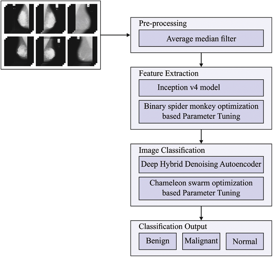
Figure 1: Overall process of HTDHDAE-BCC approach

2.1 Feature Extraction Using Inception v4

In this work, the Inception v4 model is employed to generate feature vectors. CNNs remove the need for manual extraction of features to identify features employed for classifying images. CNN operates through the extraction of features straightforwardly from images. Inception-v4 was a CNN structure constructed on earlier iterations of the Inception family by facilitating the structure and utilizing more inception modules instead of Inception-v3 [17]. The inception module has been initially presented in GoogLeNet and Inception-v1. The input went through 1 × 1, 3 × 3, and 5 × 5 conv, along with the max pooling concurrently and concatenated as output. The inception-v4 presented as a Batch normalization (BN), in which ReLU can be utilized as an activation function for addressing the saturation issue and the resultant vanishing gradients. Moreover, 5 × 5 conv has been replaced by dual 3 × 3 convs for parameter minimization while keeping the receptive field size. Additionally, a factorization idea was presented in the convolution layer to diminish the dimensionality to lessen the overfitting complexity.

2.2 Hyperparameter Tuning Using BSMO Algorithm

To optimally modify the hyperparameters related to the Inception v4 model, the BSMO algorithm is utilized. SMO discovers novel solutions and uses present solutions to accomplish optimum outcomes [18]. The summary of different stages associated with the traditional SMO process is demonstrated for the reader’s rapid reference. The logical operators such as AND ( ⊗),  OR (+ ), and XOR (⊕) are applied in the SMO equation to form binary SMO as follows.

Initialization phase

Initialization of the arbitrary binary solution is as follows:

SMij={0, if x≤p1, otherwise (1)

In Eq. (7), SMij denotes the ith monkey’s jth parameter. p indicates the likelihood taken as 0.5, and x indicates an arbitrary number within [0, 1] . The dimension becomes 0 once the arbitrary value is lesser than 0.5. The logical operator upgrades afterwards initialization, the position of the SM.

Local leader (LL) stage (LLS)

SMnewij={SMij⊕((b⊗(LL_kj⊕SM_ij))+(d⊗(SM_rj⊕SM_ij))),if b≥prSMij,otherwise. (2)

In Eq. (8), SMnewij represents the upgraded location of ithSM ,  LLkj denotes the kth local group leader in the jth parameter, SMrj indicates rth SM in jth variable so that r≠i; b and d denotes binary arbitrary numbers amongst [0, 1]. pr denotes the perturbation rate.

Global leader stage (GLS)

SMnewij=SMij⊕((b⊗(GLkj⊕SMij))+(d⊗(SMrj⊕SMij))), ifb<probi (3)

Now, GLkj indicates the kth GL in the jth parameter. The updated location depends on the following formula:

probi=0.9×fitimaxfit+0.1 (4)

In Eq. (4), probi denotes the probability, fiti indicates the fitness of ith SM, and maxflt shows the maximal fitness of the group.

Local leader decision stage (LLDS)

SMnewij={SMij⊕((b⊗(LLkj⊕SMij))+(b⊗(GLj⊕SMij)))if b≥pruse Equation l2,  otherwise.  (5)

In Eq. (5), LLkj indicates the kth LL in the jth parameter, and GLj denotes GL in the jth variable.

Global leader decision stage (GLDS)

Once the GL SM value isn’t changed to global leader limit (GLL) time, GL divides the entire group into subcategories. Once the class number is equivalent to the maximal group (MG) value, then it is regarded that the maximal potential subgroup has been generated. Next, GL integrates each subgroup to generate a single group. The position of LL is eventually upgraded.

2.3 BC Classification Using Optimal DHDAE Model

For BC classification, the DHDAE model is exploited in this study. The autoencoder (AE) variants of the Deep Hybrid Boltzmann Machine (DHBM), the DHDAE, Follow the same path as a preceding subsection; however, it starts from the HSDA basis structural design [19]. Also, this borrows the similar structure of DHBM, containing the bi-direction connection required for integrating bottom-up and top-down influences. But, rather than learning through a Boltzmann-based method, we intend to learn a stochastic decoder and encoder procedure over several layers conjointly. The DHDAE might be stacking a strongly incorporated hybrid denoising autoencoder (HdA) with the coupled predictor. An HdA is a single hidden-layer MLP that shares input-to-hidden weight with an encoder-decoder module whose weight is tied (viz., decoding weight is equivalent to the transfer of encoding weight).

A 3-layer form of the joint models (generalized to L layer and determined as the similar variable set as DHBM) is quantified as the encoder (fθ1(y,  X^, h2^),  fθ2(h1^)}) and decoder (gθ(h1^)) functions:

h1=fθ1(X^,  h2^)=ϕ(W1X+(W2)Th^) (6)

h2=fθ2(h1^)=ϕ(W2h^1) (7)

x¯=gθ(h1^)=ϕ((W1)Th^1) (8)

{W1,  W2} denotes the weight matrix interconnecting input X to h1 and h1 to h2 correspondingly (the superscript T signifies a matrixes transpose function). The output operation oθ(y|h1,  h2) required to produce prediction is evaluated through Eq. (6), similar to the DHBM method. Similar to HSDA, the DHDAE exploits a stochastic mapping function h^tl∼qD(h^tl|h) for corrupting input vector (haphazardly masking entry in provided likelihood) 4 Noted that the DHDAE needs lesser matrix operation when compared to the DHBM because it exemplified the “weak multiple level semi-supervised hypotheses”, providing it with the benefit of a speedup in comparison with the DHBM.

The information flow to collect layer-by-layer statistics is specified as the arrows (that characterize an operation like element-wise non-linearity and matrix multiplication), using the vector at the arrow origin and the suitable layer parameter matrix) that is totalled based on the consecutive computation step taken to evaluate them. Arrows (or operations) in similar computation steps are similar and point to the resultant activation value evaluated. v corresponds to the detection network (Qrec) primary guess for the mean-field, whereas μ characterizes the real mean-field statistics. Fig. 2 showcases the infrastructure of AE.

Figure 2: Structure of autoencoder

To evaluate layer-by-layer activation value for the DHDAE, one uses the detection model to attain primary guess for {h1,  h2} .

For optimal hyperparameter tuning of the DHDAE, the CSO algorithm is used. CSO algorithm stimulates the hunting and food-searching method [20]. They are many specified classes of species that can change colour to blend with their surroundings. They can live and survive in semi-desert areas, lowlands, mountains, and deserts and usually eat insects. The food hunting procedure includes the following phases: attacking, tracking, and pursuing the prey using their sight. The mathematical steps and models are described in the succeeding subsections.

CSO algorithm was a population-related meta-heuristic that arbitrarily produces an initializing population to begin the optimization procedure. The chameleon population having the size n was generated in a d -dimension search region in which every individual of the population becomes a feasible solution to the optimization issue. The position of the chameleon at iteration in the searching region can be considered as follows:

yti=[yt,1i, yt,2i, yt,di] (9)

where i=1, 2…t characterizes the iteration count, yτ,Error::0x0000i characterizes the chameleon location.

The initialized population is produced according to the problem dimension, and the chameleon count in the searching region is shown below:

yi=lj+r(uj−lj) (10)

In Eq. (10), yi represents the primary vector of i - th chameleons, uj and lj denote the upper and lower bounds of the searching region, correspondingly, and r shows a uniformly distributed value ranges from [0, 1]. The solution quality in every step can be evaluated for every novel location according to the assessment of objective function.

The chameleon movement behaviour in searching is represented according to the updated approach of location as follows:

yt+1i+j={yti,j+P1(Pτi,j−Gτj)r2+P2(Gτj−yτi,j)r1 yti ,j+μ(uj−lj)r3+lbjsn(rand−0.5)r1<Ppr1≥Pp (11)

In Eq. (11), t and (t+1) designate the tth and (t+1)th iterative phase correspondingly. i and j characterize the ith chameleons in the jth parameter. yti,j and yt+1i+j denote the existing and novel locations, correspondingly. Pti,j and Gtj suggest the finest and global finest locations, correspondingly.

Where P1 and P2 refer to a positive number that controls exploration capability. r1 , r2,  and r3 indicate uniformly distributed arbitrary values ranging from [0, 1]. ri denotes a uniform distribution value generated at index i ranges from [0, 1]. Pp shows the probability of the chameleon perceiving prey. Sgn(rand-0.5) denotes an effect on the direction of exploration and exploitation, and it ranges from [ −1 , 1]. μ indicates a function of the iteration variable, which decreases with iteration count.

Chameleon’s Eyes Rotation able to recognize prey location by rotating their eyes, and that feature assists in spotting the target via 360 degrees steps are given below:

•   The initial location was the focal point of gravity;

•   The rotation matrix was found out that identifies the prey position;

•   The situation is refreshed through a rotation matrix at the focal point of gravity;

•   At last, they were resumed to the initial location position

Chameleon assaults its target once it excessively comes closer. The chameleon adjacent to the target is the optimum chameleon and is regarded as the optimum outcome. Such chameleons assault the target through the tongue. The chameleon situation is enhanced since it could prolong the tongue by double the length. It assists the chameleon in exploiting the pursuit space and enables them to catch the target sufficiently. The speed of the tongue, once it is protracted toward the target, is arithmetically given as follows:

vt+1i,j=wvti,j+c1(Gtj−yti,j)+c2(Pti,j−yti,j)r2 (12)

In Eq. (12), vt+1i,j denotes the novel velocity of ith chameleons in the jth parameter of t+1 iteration, and vti,j shows the existing velocity of ith chameleon in the jth parameter.

3  Experimental Validation

The experimental validation of the HTDHDAE-BCC method is tested utilizing the MIAS dataset. It contains 322 images under three class labels, as depicted in Table 1. A few sample images are demonstrated in Fig. 3.

Figure 3: Sample images (a) Normal, (b) Benign, and (c) Malignant

Fig. 4 exhibits the confusion matrices generated by the HTDHDAE-BCC model under five runs. On run-1, the HTDHDAE-BCC model categorized 62 samples into benign, 49 into malignant, and 207 samples into normal. Temporarily, on run-2, the HTDHDAE-BCC approach has categorized 62 samples into benign, 48 samples into malignant, and 207 samples into normal. Meanwhile, on run-3, the HTDHDAE-BCC technique has categorized 62 samples into benign, 48 samples into malignant, and 209 samples into normal. Finally, on run-4, the HTDHDAE-BCC algorithm has categorized 62 samples into benign, 49 samples into malignant, and 206 samples into normal.

Figure 4: Confusion matrices of HTDHDAE-BCC approach (a) Run1, (b) Run2, (c) Run3, (d) Run4, and (e) Run5

Table 2 provides detailed BC classification outcomes of the HTDHDAE-BCC model under five distinct runs.

Fig. 5 provides the overall classifier results of the HTDHDAE-BCC model on run-1. The figure shows that the HTDHDAE-BCC model has enhanced results under all classes. For instance, the HTDHDAE-BCC model has categorized benign images with accuy , sensy , specy , Fscore , and Gmean of 100%, 100%, 100%, 100%, and 100%, respectively. Further, the HTDHDAE-BCC technique has categorized malignant images with accuy , sensy , specy , Fscore , and Gmean of 98.76%, 96.06%, 99.26%, 96.08%, and 97.66% correspondingly. In the meantime, the HTDHDAE-BCC technique has categorized normal images with accuy , sensy , specy , Fscore , and Gmean of 98.76%, 99.04%, 98.23%, 99.04%, and 98.64% correspondingly.

Figure 5: Result analysis of HTDHDAE-BCC approach under run-1

Fig. 6 presents the complete classifier results of the HTDHDAE-BCC method on run-2. The figure displayed the HTDHDAE-BCC approach has offered enhanced results under all classes. For example, the HTDHDAE-BCC methodology has categorized benign images with accuy , sensy , specy , Fscore , and Gmean of 100%, 100%, 100%, 100%, and 100%, respectively. Additionally, the HTDHDAE-BCC technique has categorized malignant images with accuy , sensy , specy , Fscore , and Gmean of 98.45%, 94.21%, 99.26%, 95.05%, and 96.66%, respectively. Meanwhile, the HTDHDAE-BCC algorithm has categorized normal images with accuy , sensy , specy , Fscore , and Gmean of 98.45%, 99.04%, 97.35%, 98.81%, and 98.19% correspondingly.

Figure 6: Result analysis of HTDHDAE-BCC approach under run-2

Fig. 7 illustrates the inclusive classifier results of the HTDHDAE-BCC technique on run-3. The figure represented the HTDHDAE-BCC approach has presented enhanced results under all classes. For example, the HTDHDAE-BCC method has categorized benign images with accuy , sensy , specy , Fscore , and Gmean of 100%, 100%, 100%, 100%, and 100%, correspondingly. Moreover, the HTDHDAE-BCC methodology has categorized malignant images with accuy , sensy , specy , Fscore , and Gmean of 99.07%, 94.12%, 100%, 96.97%, and 97.01% correspondingly. In parallel, the HTDHDAE-BCC approach has categorized normal image with accuy , sensy , specy , Fscore , and Gmean of 99.07%, 100%, 97.35%, 99.29%, and 98.66% correspondingly.

Figure 7: Result analysis of HTDHDAE-BCC approach under run-3

Fig. 8 portrays the general classifier results of the HTDHDAE-BCC methodology on run-4. The figure denoted the HTDHDAE-BCC technique has provided enhanced results under all classes. For example, the HTDHDAE-BCC approach has categorized benign images with accuy , sensy , specy , Fscore , and Gmean of 99.69%, 100%, 99.62%, 99.20%, and 99.81% correspondingly. Further, the HTDHDAE-BCC algorithm has categorized malignant images with accuy , sensy , specy , Fscore , and Gmean of 99.76%, 96.08%, 99.26%, 96.08%, and 97.66% correspondingly. In the meantime, the HTDHDAE-BCC technique has categorized normal images with accuy , sensy , specy , Fscore , and Gmean of 98.45%, 98.56%, 98.23%, 98.80%, and 98.40% correspondingly.

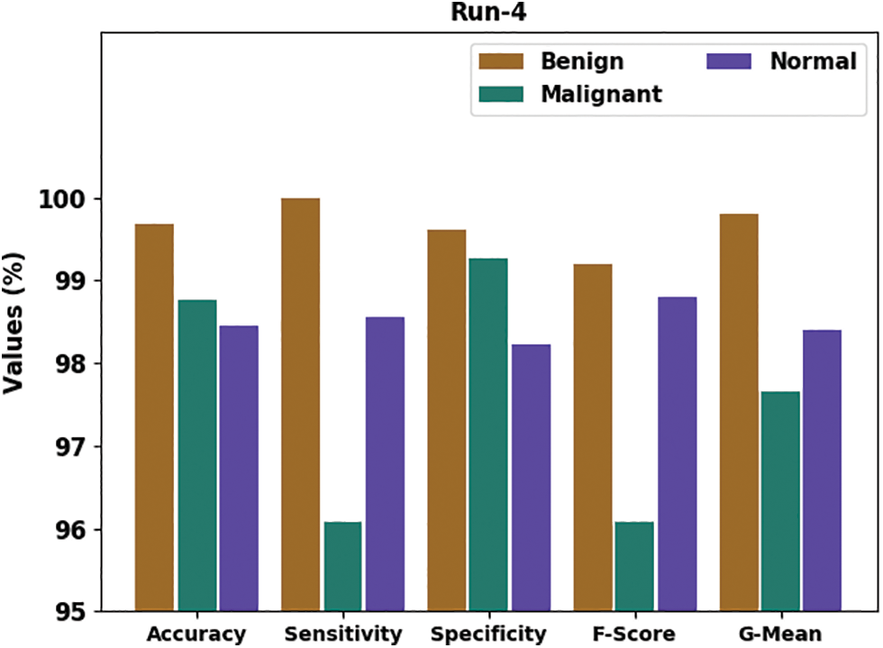
Figure 8: Result analysis of HTDHDAE-BCC approach under run-4

Fig. 9 delivers an overall classifier fallout of the HTDHDAE-BCC approach on run-5. The figure exemplified the HTDHDAE-BCC methodology has rendered enhanced results under all classes. For example, the HTDHDAE-BCC algorithm has categorized benign images with accuy , sensy , specy , Fscore , and Gmean of 100%, 100%, 100%, 100%, and 100% correspondingly. Additionally, the HTDHDAE-BCC method has categorized malignant images with accuy , sensy, specy , Fscore , and Gmean of 98.45%, 98.04%, 98.52%, 95.24%, and 98.28% correspondingly. In the meantime, the HTDHDAE-BCC approach has categorized normal image with accuy , sensy , specy , Fscore , and Gmean of 98.45%, 98.09%, 99.12%, 98.80%, and 98.60% correspondingly.

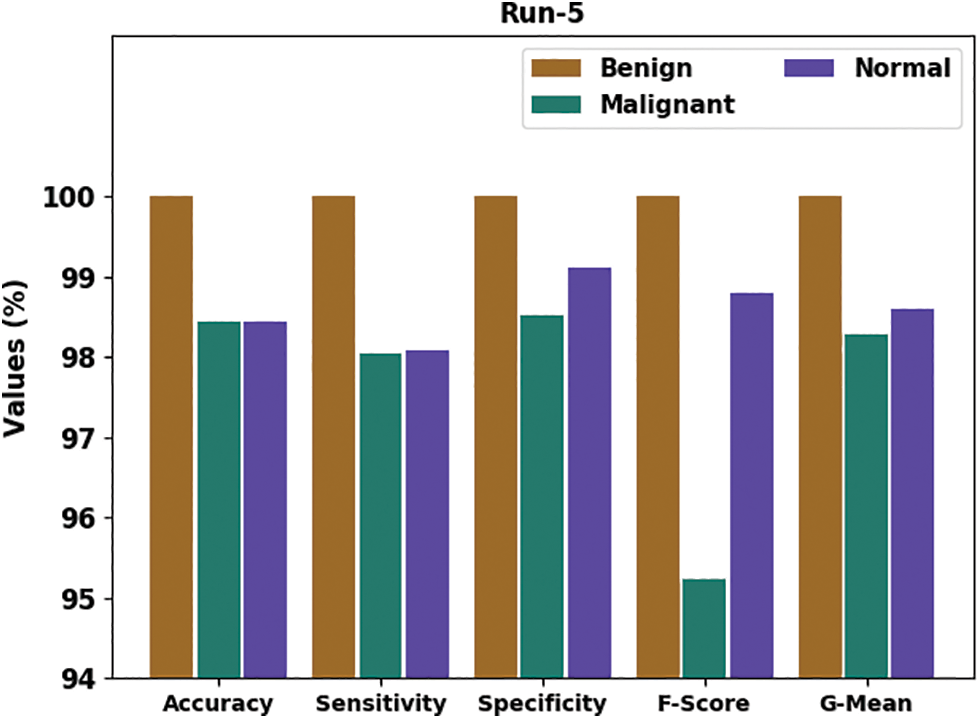
Figure 9: Result analysis of HTDHDAE-BCC approach under run-5

Fig. 10 demonstrates the average classification outcomes of the HTDHDAE-BCC model. On run-1, the HTDHDAE-BCC model has attained average  accuy , sensy , specy , Fscore , and Gmean of 99.17%, 98.37%, 99.16%, 98.37%, and 98.76% respectively. In line with, on run-2, the HTDHDAE-BCC approach has gained average  accuy , sensy , specy , Fscore , and Gmean of 98.96%, 97.92%, 98.87%, 97.95%, and 98.28% correspondingly. Additionally, on run-4, the HTDHDAE-BCC model has obtained average  accuy , sensy , specy , Fscore , and Gmean of 98.96%, 98.21%, 99.04%, 98.03%, and 98.62%, correspondingly. At last, on run-5, that the HTDHDAE-BCC approach has reached average  accuy , sensy , specy , Fscore , and Gmean of 98.96%, 98.71%, 99.21%, 98.01%, and 98.96% correspondingly.

Figure 10: Average analysis of HTDHDAE-BCC approach (a) Run1, (b) Run2, (c) Run3, (d) Run4, and (e) Run5

The training accuracy (TRA) and validation accuracy (VLA) obtained by the HTDHDAE-BCC method on the test dataset is illustrated in Fig. 11. The experimental outcome inferred that the HTDHDAE-BCC technique had achieved maximal values of TRA and VLA. Particularly the VLA seemed to be higher than TRA.

Figure 11: TRA and VLA analysis of HTDHDAE-BCC approach

The training loss (TRL) and validation loss (VLL) achieved by the HTDHDAE-BCC approach on the test dataset are established in Fig. 12. The experimental outcome implied that the HTDHDAE-BCC algorithm had accomplished the least values of TRL and VLL. In specific, the VLL is lower than TRL.

Figure 12: TRL and VLL analysis of HTDHDAE-BCC approach

A brief ROC analysis of the HTDHDAE-BCC method on the test dataset is depicted in Fig. 13. The results denoted the HTDHDAE-BCC approach has shown its ability to categorize distinct classes on the test dataset.

Figure 13: ROC analysis of HTDHDAE-BCC approach

To ensure the enhanced results of the HTDHDAE-BCC model, a brief comparative examination is offered in Table 3 [21]. The outcomes inferred the improved outcomes of the HTDHDAE-BCC model compared to existing techniques. Based on accuy , the HTDHDAE-BCC model has offered a higher accuy of 99.38%, whereas the deep computer-aided diagnosis (deep-CAD), CNN, improved CNN, Opt. DL and DL-TLT models have obtained lower accuy of 92.47%, 85.87%, 86.25%, 91.93%, and 98.90% respectively.

Simultaneously, based on sensy , the HTDHDAE-BCC model has offered a higher sensy of 98.04%, whereas the deep-CAD, CNN, improved CNN, Opt. DL and DL-TLT models have obtained lower sensy of 97.70%, 88.52%, 94.54%, 91.52%, and 97.63%, respectively. Concurrently, based on specy , the HTDHDAE-BCC model has offered a higher specy of 99.12% whereas the deep-CAD, CNN, improved CNN, Opt. DL and DL-TLT models have obtained lower specy of 88.99%, 91.46%, 94.22%, 95.63%, and 99.04%, respectively. These values ensured that the HTDHDAE-BCC model had shown effectual BC classification outcomes over existing DL models.

4  Conclusion

In this paper, a novel HTDHDAE-BCC algorithm was projected for the classification of BC on digital mammograms. In the HTDHDAE-BCC model, the initial stage of image pre-processing is carried out using an average median filter. In addition, the deep convolutional neural network-based Inception v4 model is employed to generate feature vectors. The parameter tuning process can be performed using the binary spider monkey optimization (BSMO) algorithm. The HTDHDAE-BCC model exploits the CSO algorithm with the DHDAE model for BC classification. The experimental analysis of the HTDHDAE-BCC model is performed using the MIAS database. The experimental outcomes demonstrate the betterments of the HTDHDAE-BCC model over other recent approaches. In the upcoming years, the performance of the HTDHDAE-BCC technique can be boosted by a deep instance segmentation model.

Funding Statement: This project was supported by the Deanship of Scientific Research at Prince SattamBin Abdulaziz University under research Project# (PSAU-2022/01/20287).

Conflicts of Interest: The author declares that they have no conflicts of interest to report regarding the present study.

References

1. L. Tsochatzidis, L. Costaridou and I. Pratikakis, “Deep learning for breast cancer diagnosis from mammograms—A comparative study,” Journal of Imaging, vol. 5, no. 3, pp. 37, 2019. [Google Scholar] [PubMed]

2. Y. J. Suh, J. g and B. J. Cho, “Automated breast cancer detection in digital mammograms of various densities via deep learning,” Journal of Personalized Medicine, vol. 10, no. 4, pp. 211, 2020. [Google Scholar] [PubMed]

3. A. Akselrod-Ballin, M. Chorev, Y. Shoshan, A. Spiro, A. Hazan et al., “Predicting breast cancer by applying deep learning to linked health records and mammograms,” Radiology, vol. 292, no. 2, pp. 331–342, 2019. [Google Scholar] [PubMed]

4. L. Shen, L. R. Golies, J. H. Rothstein, E. Fluder, R. McBride et al., “Deep learning to improve breast cancer detection on screening mammography,” Scientific Reports, vol. 9, no. 1, pp. 1–12, 2019. [Google Scholar]

5. A. Kumar, S. Mukherjee and A. K. Luhach, “Deep learning with perspective modeling for early detection of malignancy in mammograms,” Journal of Discrete Mathematical Sciences and Cryptography, vol. 22, no. 4, pp. 627–643, 2019. [Google Scholar]

6. C. D. Lehman, A. Yala, T. Schuster, B. Dontchos, M. Bahl et al., “Mammographic breast density assessment using deep learning: Clinical implementation,” Radiology, vol. 290, no. 1, pp. 52–58, 2019. [Google Scholar] [PubMed]

7. X. Zhu, T. K. Wolfgruber, L. Leong, M. Jensen, C. Scott et al., “Deep learning predicts interval and screening-detected cancer from screening mammograms: A case-case-control study in 6369 women,” Radiology, vol. 301, no. 3, pp. 550–558, 2021. [Google Scholar] [PubMed]

8. D. Arefan, A. A. Mohamed, W. A. Berg, M. L. Zuley, J. H. Sumkin et al., “Deep learning modeling using normal mammograms for predicting breast cancer risk,” Medical Physics, vol. 47, no. 1, pp. 110–118, 2020. [Google Scholar] [PubMed]

9. W. Lotter, A. R. Diab, B. Haslam, J. G. Kim, G. Grisot et al., “Robust breast cancer detection in mammography and digital breast tomosynthesis using an annotation-efficient deep learning approach,” Nature Medicine, vol. 27, no. 2, pp. 244–249, 2021. [Google Scholar] [PubMed]

10. S. S. Chakravarthy and H. Rajaguru, “Automatic detection and classification of mammograms using improved extreme learning machine with deep learning,” IRBM, vol. 43, no. 1, pp. 49–61, 2022. [Google Scholar]

11. G. Altan, “Deep learning-based mammogram classification for breast cancer,” International Journal of Intelligent Systems and Applications in Engineering, vol. 8, no. 4, pp. 171–176, 2020. [Google Scholar]

12. S. A. A. Hassan, M. S. Sayed, M. I. Abdalla and M. A. Rashwan, “Breast cancer masses classification using deep convolutional neural networks and transfer learning,” Multimedia Tools and Applications, vol. 79, no. 41, pp. 30735–30768, 2020. [Google Scholar]

13. J. D. L. Cabrera, L. A. L. Rodríguez and M. P. Díaz, “Classification of breast cancer from digital mammography using deep learning,” Inteligencia Artificial, vol. 23, no. 65, pp. 56–66, 2020. [Google Scholar]

14. T. Kavitha, P. P. Mathai, C. Karthikeyan, M. Ashok, R. Kohar et al., “Deep learning based capsule neural network model for breast cancer diagnosis using mammogram images,” Interdisciplinary Sciences: Computational Life Sciences, vol. 14, no. 1, pp. 113–129, 2022. [Google Scholar] [PubMed]

15. N. Saffari, H. A. Rashwan, M. A. Nasser, V. K. Singh, M. Arenas et al., “Fully automated breast density segmentation and classification using deep learning,” Diagnostics, vol. 10, no. 11, pp. 988, 2020. [Google Scholar] [PubMed]

16. S. Zahoor, U. Shoaib and I. U. Lali, “Breast cancer mammograms classification using deep neural network and entropy-controlled whale optimization algorithm,” Diagnostics, vol. 12, no. 2, pp. 557, 2022. [Google Scholar] [PubMed]

17. M. A. S. Al Husaini, M. H. Habaebi, T. S. Gunawan, M. R. Islam, E. A. Elsheikh et al., “Thermal-based early breast cancer detection using inception V3, inception V4 and modified inception MV4,” Neural Computing and Applications, vol. 34, no. 1, pp. 333–348, 2022. [Google Scholar] [PubMed]

18. N. Khare, P. Devan, C. L. Chowdhary, S. Bhattacharya, G. Singh et al., “Smo-dnn: Spider monkey optimization and deep neural network hybrid classifier model for intrusion detection,” Electronics, vol. 9, no. 4, pp. 692, 2020. [Google Scholar]

19. A. G. Ororbia II, C. L. Giles and D. Reitter, “Online semi-supervised learning with deep hybrid boltzmann machines and denoising autoencoders,” arXiv preprint arXiv:1511.06964, 2015. [Google Scholar]

20. M. Said, A. M. El-Rifaie, M. A. Tolba, E. H. Houssein and S. Deb, “An efficient chameleon swarm algorithm for economic load dispatch problem,” Mathematics, vol. 9, no. 21, pp. 2770, 2021. [Google Scholar]

21. A. Saber, M. Sakr, O. M. Abo-Seida, A. Keshk and H. Chen, “A novel deep-learning model for automatic detection and classification of breast cancer using the transfer-learning technique,” IEEE Access, vol. 9, pp. 71194–71209, 2021. [Google Scholar]