
 Submit a Paper
 Propose a Special lssue
 Open Access
ARTICLE

Approximations by Ideal Minimal Structure with Chemical Application
1 Department of Mathematics, Faculty of Science, Zagazig University, Zagazig, 44519, Egypt
2 Department of Mathematics, Faculty of Science, Zarqa University, Zarqa, 13132, Jordan
3 Department of Mathematics, Faculty of Science, Tanta University, Tanta, 31527, Egypt
* Corresponding Author: Mostafa K. El-Bably. Email:
Intelligent Automation & Soft Computing 2023, 36(3), 3073-3085. https://doi.org/10.32604/iasc.2023.034234
Received 11 July 2022; Accepted 26 October 2022; Issue published 15 March 2023
 View Full Text
 Download PDF
Abstract
The theory of rough set represents a non-statistical methodology for analyzing ambiguity and imprecise information. It can be characterized by two crisp sets, named the upper and lower approximations that are used to determine the boundary region and accurate measure of any subset. This article endeavors to achieve the best approximation and the highest accuracy degree by using the minimal structure approximation space via ideal . The novel approach (indicated by ) modifies the approximation space to diminish the boundary region and enhance the measure of accuracy. The suggested method is more accurate than Pawlak’s and EL-Sharkasy techniques. Via illustrated examples, several remarkable results using these notions are obtained and some of their properties are established. Several sorts of near open (resp. closed) sets based on are studied. Furthermore, the connections between these assorted kinds of near-open sets in are deduced. The advantages and disadvantages of the proposed approach compared to previous ones are examined. An algorithm using MATLAB and a framework for decision-making problems are verified. Finally, the chemical application for the classification of amino acids (AAs) is treated to highlight the significance of applying the suggested approximation.Keywords
Topological structures and their generalizations are of crucial importance in data analysis, which have manifested in different fields, for example, in physics [1], chemistry [2], medicine [3], soft set theory [4], etc. Lashin et al. [5] used topological notions to study different issues in rough set theory in order to generalize Pawlak’s concepts [6] in different applications and integrate the concepts of rough and fuzzy sets. Topological structures were applied in rough sets to improve evolutionary-based feature selection technique using the extension of knowledge [7], decision making of COVID-19 [8,9], and enhanced feature selection based on integration containment neighborhoods rough set approximations and binary honey badger optimization [10]. Several articles [11–19] extended the application fields of Pawlak’s model. Popa et al. introduced the minimal structure spaces [20], as a generalization of topological spaces to analyze information systems. Various consequences of minimal spaces can be viewed in [21]. EL-Sharkasy [22,23] studied several sorts of sets in minimal structure spaces with some of their characterizations. The notion of the ideal
The main contributions of this work are constructing ideal minimal structure approximation space
Herein, some vital concepts and results are introduced, which are helpful in the sequel.
Definition 1 [13] Consider the binary relation
Definition 2 [13] Suppose that
Definition 3 [22,23] For any approximation space
(i) the minimal structure of
(ii) the elements of
(iii) the class of all
Definition 4 [22,23] Let
(i) the minimal lower approximation of
(ii) the minimal upper approximation of
(iii) the minimal accuracy of
Proposition 1 [22] If
Definition 5 [23] A subset
(i)
(ii)
(iii)
The sets of all
3 Generalized Rough Approximations Relying on Minimal Structure and Ideals
This section aims to introduce the ideal minimal structure approximation space
Definition 6 Let
(i) a minimal lower approximation
(ii) a minimal upper approximation
(iii) a minimal accuracy
Remark 1 When
To study the prime properties of
Proposition 2 For an
(i)
(ii)
(iii) if
(iv)
(v)
Proof. The first item will be proved, and the others similarly.
Example 1 Let
Hence,
Remark 2 Example 1 represents the following:
(i) the inversion of statement (iii) from Proposition 2 is not true. Suppose
(ii) the inclusion of the first part of the statement (iv) of Proposition 2 cannot be exchanged by an equality symbol. Suppose
(iii) the inclusion of the second part of the statement (iv) of Proposition 2 cannot be exchanged by equality symbol. Suppose
(iv) the inclusion of the first part of the statement (v) of Proposition 2 cannot be exchanged by equality symbol. Consider
(v) the inclusion of the second part of the statement (v) of Proposition 2 cannot be exchanged by equality symbol. Consider
The succeeding proposition is realized depending on Proposition 1.
Proposition 3 Let
The next remark is devoted to clarifying the differences between the existing approximations and the preceding one of Propositions 2 & 3 in [22].
Remark 3 Let
(i)
(ii)
(iii)
(iv)
Proposition 4 Let
(i) if
(ii) if
(iii)
(iv)
(v)
(vi)
Proof. The first item will be proved, and the others similarly.
Let
Example 2 Let
Remark 4 Suppose
(i) the inversion of statement (i) from Proposition 4 is false. Suppose
(ii) the inversion of statement (ii) from Proposition 4 is not true. Suppose
Consequently, for any relation, the new kind of rough approximations
Remark 5 Table 1 compare between lower approximations, upper approximations, and the accuracy and Table 2 compare between boundary, internal edge, and external edge defined in Definitions 4 and 6 which are given by the relation
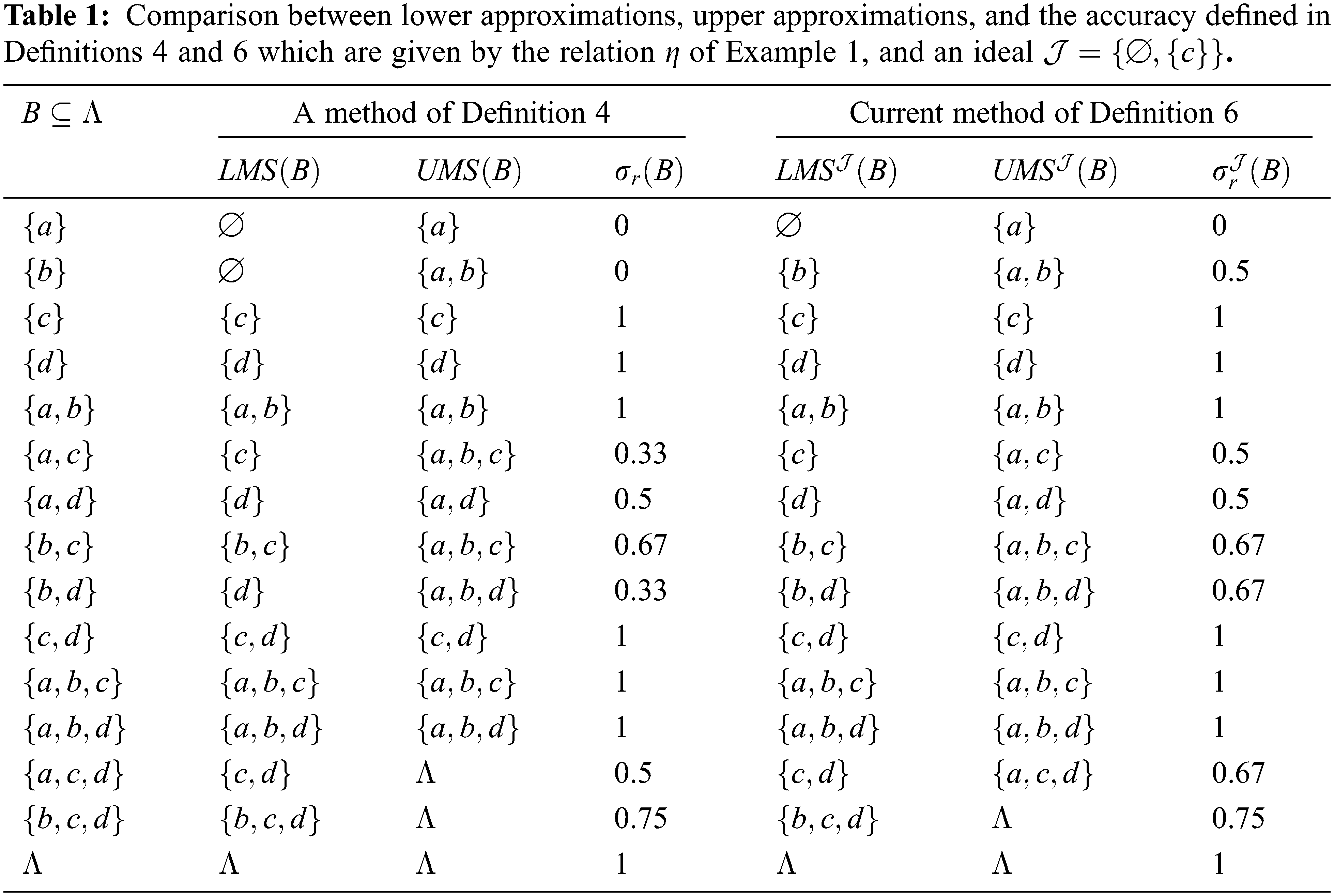
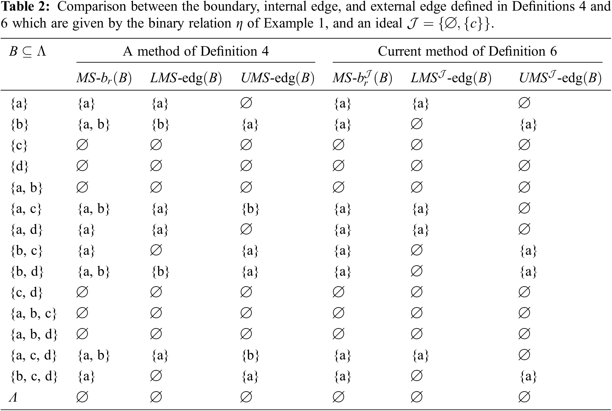
The next result exhibits the connections among the lower, and upper approximations and the degree of accuracy that were offered in both Definitions 4, and 6.
Theorem 1 Let
(i)
(ii)
(iii)
Proof. The first item will be proved, and the others similarly.
Let
Remark 6 It must be perceived that the suggested approximations
(i)
(ii)
Definition 7 For an
(i) a minimal positive of
(ii) a minimal exterior (negative) of
(iii) a minimal boundary of
(iv) a minimal internal edge of
(v) a minimal external edge of
Remark 7 According to Example 1 with
(i)
(ii)
(iii)
Definition 8 For an
(i)
(ii)
(iii)
Remark 8 According to Table 1 and Example 1 with
(i) the sets
(ii) the sets
(iii) the sets
Corollary 1 For a
(i) every
(ii) every
4 Some Near Open Sets Based on MSAS and Ideals
This section aims to introduce and investigate some sorts of near open (resp. closed) sets via the viewpoint of an
Definition 9 A subset
(i)
(ii)
(iii)
Remark 9
(i) The complement of an
(ii) The set of all
Remark 10 In a topological space, the class of semi (resp. pre-) open sets is contained in the class of ideal semi (resp. pre-) open sets. While this fact is discussed for minimal structures, surprisingly it is incorrect i.e.,
Example 3 (Continued from Example 2) Consider
(i)
(ii)
(iii)
(iv)
(v)
(vi)
Example 4 Consider
(i)
(ii)
(iii)
(iv)
(v)
(vi)
(vii)
(viii)
(ix)
According to Definition 9, the proof of the proposition 5 is obvious.
Proposition 5 Let
The next example shows that the converse of Proposition 5 is incorrect.
Example 5 In Example 4,
Remark 11 In view of Example 4, the following results are noticed:
(i) the union of
(ii) the intersection of
(iii) the intersection of
(iv) the intersection of
(v) the intersection of
(vi) the intersection of
An example in the area of chemistry is provided by utilizing the actual approximation in Definition 6 to clarify the notions practically.
Example 6 [26] Let
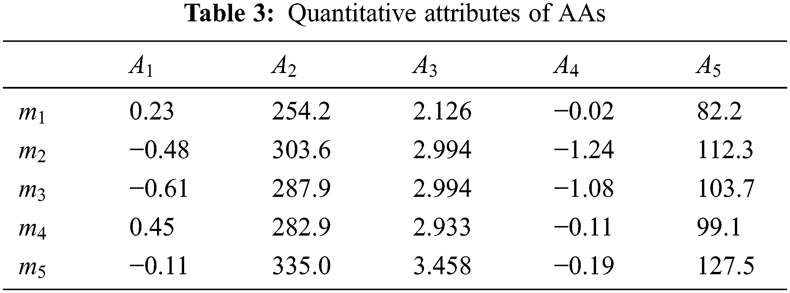
Presently, it shall be investigated five relations on
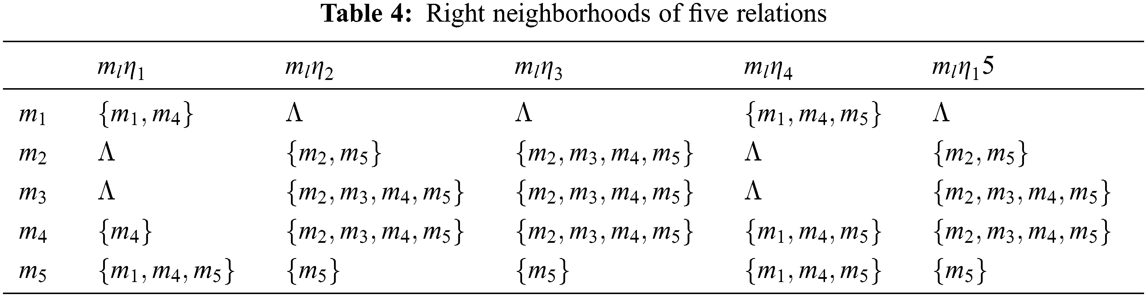
The intersection of all right neighborhoods of all elements
If
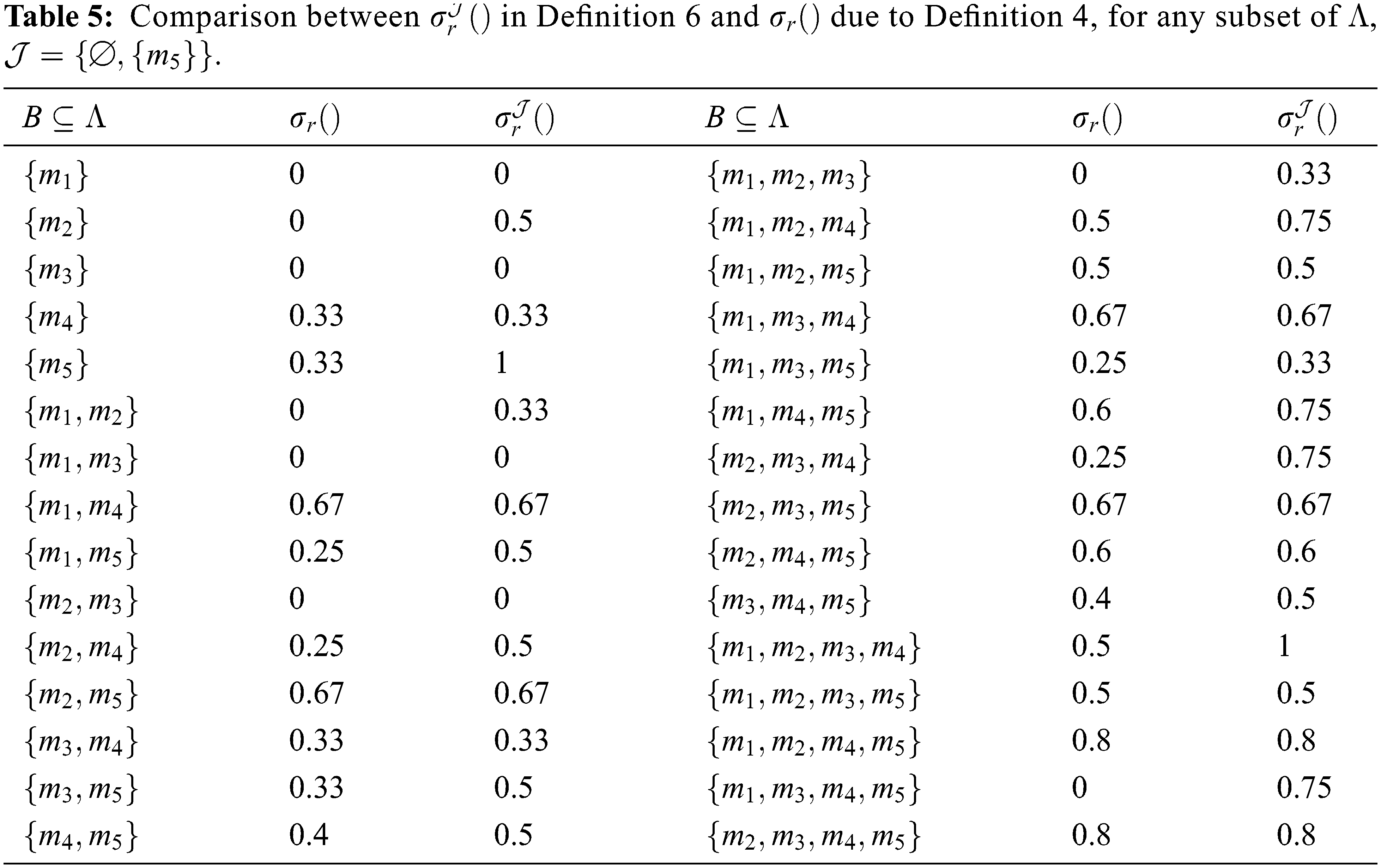
The ideal minimal accuracy measure
This section provides an algorithm and a framework for decision-making problems. The suggested algorithm is checked with fictitious data and compared to existing methods. This technique represents a simple tool that can be used in MATLAB.
Require: Initiate an information table generated from the given data such that the first column contains a set of objects
Output: An accurate decision for exact and rough sets.
Step 1: Input a finite set of data as a universal set
Step 2: Define the binary relations
Step 3: Compute all right neighborhoods of all elements by
Step 4: Construct the class of minimal structure by Step 3.
Step 5: Using the ideal
Step 6: Using the ideal
Step 7: If
The following figure (Fig. 1) illustrates a simple flowchart for calculating the degree of accuracy induced from the above algorithm.

Figure 1: A flowchart for decision making using an
The novel rough approximation space
One of the challenges in daily problems, as in the medical diagnosis, is making an accurate decision. Therefore, the applied example in biochemistry offers a clear vision that the expansion using the ideal gives better results. Thus, by the
In the forthcoming, the
Acknowledgement: We appreciate the reviewers for their invaluable time in reviewing our paper and providing thoughtful and valuable comments. It was their insightful suggestions that led to sensible improvements in the current version.
Funding Statement: The authors received no specific funding for this study.
Conflicts of Interest: The authors declare that they have no conflicts of interest to report regarding the present study.
References
1. A. Galton, “A generalized topological view of motion in discrete space,” Theoretical Computer Science, vol. 305, no. 1–3, pp. 111–134, 2003. [Google Scholar]
2. B. Stadler and P. Stadler, “Generalized topological spaces in evolutionary theory and combinatorial chemistry,” Journal of Chemical Information and Computer Sciences, vol. 42, no. 3, pp. 577–585, 2002. [Google Scholar] [PubMed]
3. R. Abu-Gdairi, M. A. El-Gayar, T. M. Al-shami, A. S. Nawar and M. K. El-Bably, “Some topological approaches for generalized rough sets and their decision-making applications,” Symmetry, vol. 14, no. 1, pp. 95–119, 2022. [Google Scholar]
4. M. K. El-Bably, M. I. Ali and E. A. Abo-Tabl, “New topological approaches to generalized soft rough approximations with medical applications,” Journal of Mathematics, vol. 2021, no. 2559495, pp. 1–16, 2021. [Google Scholar]
5. E. F. Lashin, A. M. Kozae, A. A. Abo Khadra and T. Medhat, “Rough set theory for topological spaces,” International Journal of Approximate Reasoning, vol. 40, no. 1–2, pp. 35–43, 2005. [Google Scholar]
6. Z. Pawlak, “Rough sets,” International Journal of Computer Information Sciences, vol. 11, no. 5, pp. 341–356, 1982. [Google Scholar]
7. M. Abdelaziz, H. M. Abu-Donia, R. A. Hosny, S. L. Hazae and R. A. Ibrahim, “Improved evolutionary-based feature selection technique using extension of knowledge based on the rough approximations,” Information Sciences, vol. 594, pp. 76–94, 2022. [Google Scholar]
8. M. A. El-Gayar and A. A. E. Atik, “Topological models of rough sets and decision making of COVID-19,” Complexity, vol. 2022, no. 2989236, pp. 1– 10, 2022. [Google Scholar]
9. R. Abu-Gdairi, M. A. El-Gayar, M. K. El-Bably and K. K. Fleifel, “Two different views for generalized rough sets with applications,” Mathematics, vol. 9, no. 18, pp. 2275–2296, 2021. [Google Scholar]
10. R. A. Hosny, M. Abdelaziz and R. A. Ibrahim, “Enhanced feature selection based on integration containment neighborhoods rough set approximations and binary honey badger optimization,” Computational Intelligence and Neuroscience, vol. 2022, no. 3991870, pp. 1–17, 2022. [Google Scholar]
11. K. Qin, J. Yang and Z. Pei, “Generalized rough sets based on reflexive and transitive relations,” Information Sciences, vol. 178, no. 21, pp. 4138–4141, 2008. [Google Scholar]
12. M. Kondo, “On structure of generalized rough sets,” Information Sciences, vol. 176, no. 5, pp. 589–600, 2006. [Google Scholar]
13. Y. Y. Yao, “Two views of the theory of rough sets in finite universes,” International Journal of Approximation Reasoning, vol. 15, no. 4, pp. 291–317, 1996. [Google Scholar]
14. M. K. El-Bably and M. E. Sayed, “Three methods to generalize Pawlak approximations via simply open concepts with economic applications,” Soft Computing, vol. 26, no. 10, pp. 4685–4700, 2022. [Google Scholar]
15. M. E. Abd El-Monsef, M. A. EL-Gayar and R. M. Aqeel, “On relationships between revised rough fuzzy approximation operators and fuzzy topological spaces,” International Journal of Granular Computing, Rough Sets and Intelligent Systems, vol. 3, no. 4, pp. 257–271, 2014. [Google Scholar]
16. M. E. Abd El-Monsef, M. A. El-Gayar and R. M. Aqeel, “A comparison of three types of rough fuzzy sets based on two universal sets,” International Journal of Machine Learning and Cybernetics, vol. 8, no. 1, pp. 343–353, 2017. [Google Scholar]
17. A. T. Azar, M. S. Elgendy, M. Abdul Salam and K. M. Fouad, “Rough sets hybridization with mayfly optimization for dimensionality reduction,” Computers, Materials & Continua, vol. 73, no. 1, pp. 1087–1108, 2022. [Google Scholar]
18. A. B. Khoshaim, S. Abdullah, S. Ashraf and M. Naeem, “Emergency decision-making based on q-rung orthopair fuzzy rough aggregation information,” Computers, Materials & Continua, vol. 69, no. 3, pp. 4077–4094, 2021. [Google Scholar]
19. X. Li, S. Zhou, Z. An and Z. Du, “Multi-span and multiple relevant time series prediction based on neighborhood rough set,” Computers, Materials & Continua, vol. 67, no. 3, pp. 3765–3780, 2021. [Google Scholar]
20. V. Popa and T. Noiri, “On the definitions of some generalized forms of continuity under minimal conditions,” Kochi University, vol. 22, pp. 9–18, 2001. [Google Scholar]
21. M. Alimohammady and M. Roohi, “Linear minimal space,” Chaos, Solitons & Fractals, vol. 33, no. 4, pp. 1348–1354, 2007. [Google Scholar]
22. M. M. EL-Sharkasy, “Minimal structure approximation space and some of its application,” Journal of Intelligent & Fuzzy Systems, vol. 40, no. 1, pp. 973–982, 2021. [Google Scholar]
23. M. M. EL-Sharkasy and F. Altwme, “Some new types of approximations via minimal structure,” Journal of the Egyptian Mathematical Society, vol. 26, no. 1, pp. 287–296, 2018. [Google Scholar]
24. K. Kuratowski, Topology, vol. 1. New York: Academic Press, 1966. [Google Scholar]
25. R. A. Hosny, T. M. Al-shami, A. A. Azzam and A. S. Nawar, “Knowledge based on rough approximations and ideals,” Mathematical Problems in Engineering, vol. 2022, no. 3766286, pp. 1–12, 2022. [Google Scholar]
26. A. S. Nawar, M. A. El-Gayar, M. K. El-Bably and A. R. Hosny, “θβ-ideal approximation spaces and their applications,” AIMS Mathematics, vol. 7, no. 2, pp. 2479–2497, 2022. [Google Scholar]
27. R. A. Hosny, B. A. Asaad, A. A. Azzam and T. M. Al-shami, “Various topologies generated from Ej-neighbourhoods via ideals,” Complexity, vol. 2021, no. 4149368, pp. 1–11, 2021. [Google Scholar]
Cite This Article
 Copyright © 2023 The Author(s). Published by Tech Science Press.
This work is licensed under a Creative Commons Attribution 4.0 International License , which permits unrestricted use, distribution, and reproduction in any medium, provided the original work is properly cited.
 Downloads
 Citation Tools