Novel Vegetation Mapping Through Remote Sensing Images Using Deep Meta Fusion Model

1  Introduction

Detection of invasive species is a complex task in vegetation mapping systems. Remote sensing techniques are helpful in the invasive methods of vegetation mapping. In coastal areas, the densely turned cloud cover disturbs the process of phonological information deriving. Scene-based methods are less applicable in these areas [1]. Vegetation is crucial for global changes and plays a significant role in the carbon cycle, land-atmosphere interactions, and ecosystem maintenance. Advanced microwave scanning radiometer-earth observing system (AMSR-E) measurements are utilized for passive vegetation mapping [2].

On the other hand, vegetation mapping is also essential for soil moisture analysis using microwave remote sensing. The Radar vegetation index (RVI) is helpful in the estimation of vegetation water content (VWC). Due to frequent variations in vegetation structure and surface roughness, high-level observations are required [3]. The Convolution neural network approach is used for vegetation mapping through image recognition in buildings [4]. The author utilized the MODIS NDVI dataset in the interior location of Mongolia and China to analyze the grassland using Unmanned Aerial Vehicles (UAV). The spatial distribution and temporal grassland classification in the large coverage areas are examined. The Random Forest algorithm is utilized here, provided with the efficient Kappa Score of 0.62 and an accuracy of 72.17%. Further, the algorithm is used only for the static classification of grassland images. The work needs to be extended to include climate changes, topography, and type of soil coverage, through mapping and surveying. They were tuning hyper-parameters to help model the vegetation mapping system using digital images that attract the relevant degradation. Lower-altitude carbon images are captured using drones for mapping the vegetation area [5]. Accurate detection of vegetation mapping areas is essential to maintaining the environmental ecology. Estimating vegetation mapping in forests and densely covered areas is complex. Unique prediction alone is not enough to map the vegetation accurately. Fractional vegetation mapping is required to estimate the regular coverage in the spatial resolution method [6]. Considering the surface analysis framework in urban areas, the intensity variations and heat are monitored despite temperature changes in various zones. The presented approach defines the invaded vegetation and growth area in the selected zones by identifying the intensity variations. The presented system also captures the thermal changes using intensity mapping [7]. The standard method utilized for vegetation mapping through the NDVI technique is discussed. The concept of NDVI lies in the process of plant reflections that respond to infrared light, where the visible light strongly determines the plant’s photosynthesis. The measure of the index is helpful in two ways to stop calibrated results helpful in understanding the vegetation growth and mapping of vegetation area that is highly dense in specific features [8].

The Research Perspectives of this paper are as follows:

1.    To protect the land surfaces, it is important to utilize the resources and map the vegetation areas. Globally mapping the various vegetation spaces enable the proper utilization of resources. Interpreting and mapping locations are essential to safeguard the unauthorized vegetation area, water resources, surfaces, and crop cultivation areas.

2.    Further, keeping these constraints as the research motive, the goal of the proposed system is formulated with deep extraction of regions to be utilized for vegetation using eMODIS NDVI dataset from earth explorer. The proposed framework is modelled with three different phases of feature study using Region-based features, Unique covariate-based features and Intensity-based features etc., to map the regions globally.

3.    Various statistical measures are made and compared with the existing system in terms of the accuracy of the Kappa score, and a formulated confusion matrix is derived.

The rest of the Paper is structured with a Background study relevant to the existing research in Section 2 and followed by the system design frameworks discussed in Section 3. The research is based on existing drawbacks discussed in the background study and sorting out the problem statement defined in the system design section. Detailed design architecture and methodology of implementation are discussed in Section 4. Various results are briefly discussed in Section 5 followed by the Conclusion of the research paper with future extensions.

2  Background Study

Urban vegetation mapping using deep neural network is significantly explained with stopper explainable AI (XAI) can help different insights of training data set. This method evaluates the vegetation area from the given data set. This classification process uses aerial imagery based on spectral and textural features and achieves an accuracy of 94.4% for vegetation cover mapping. This study also reveals that spectral characteristics are insufficient for mapping vegetation coverage [9]. The multi-temporal downscaled imaging technique is available in the present system. Spatial heterogeneity in soil shows the vegetation area. Images are downscaled to account for spatial heterogeneity using rapid eye images. The downscaling technique of vegetation mapping evaluated the results. The process helps maintain low cost and hiring coverage of vegetation mapping. The proposed random forest classifier (RFC) achieved an accuracy of 92.4% [10]. A Bilateral extended short-term memory network is created for vegetation index mapping using European standard agricultural policy. Recurrent neural networks and convolutional neural networks help predict the vegetation mapping area with accurate interpretation. Given static information using the temporal values, an adaptive back-propagation process in Long Short Term Memory (LSTM) accuracy of 99% is achieved. This method helps analyze the behaviour of deep learning models in agricultural applications [11]. The author presented a deep learning approach using DeepLabV3+ customized with convolution neural network architecture. The NVDI dataset, based on RGB colour feature extraction, achieved the detection and mapping accuracy of 86% [12]. Utilizing the LandSat dataset with a convolution neural network, the vegetation mapping model achieves an accuracy of 97%. Based on precision and mapping, increased validation score, the vegetation is observed with 0.53 to 0.83 precisions [13]. The author presented a framework using the Google earth engine (GEE) images’, using multi-spectral satellite captures. Collecting various multi-spectral images from NVDI, Landsat, BEVI, and BSI, combined with GEE, the most frequent occurrence of Spectral correlations are mapped. The proposed approach attained an accuracy of 86% with an RMSE of 0.09. The method is helpful for the distribution of forest resources that are densely covered in the specified locations. In a further expansion of the work, suggest improving the accuracy by exploring more spatial resolution images and modelling new, improved accuracy [14]. The author discussed the remote sensing images-based water use efficiency in the specified region. Through the evapotranspiration method, the spatial mapping of water resources has collaborated. The mean error rate of 4.3% is formulated. The presented approach achieved a kappa coefficient of 0.86, and an RMSE of 0.52 is achieved [15].

2.1 Problem Definition

Due to the significant changes in climate and environment, various earth locations are changing, and many resources, such as water resources and vegetation, are not visible for utilization. Remotely sensed images are available in a massive collection, helpful for mapping the vegetation area correctly and accurately to use it to the maximum. Resources such as water resources, vegetation resources, different soil types, and cultivation lands are left untreated because of locating the pathways and features of the natural behaviour. The proposed study considers how vegetation mapping from remotely sensed images can help make use of the land, and surface area, for the benefit of everyone to safeguard the environment and natural resources.

2.2 Datasets Available

SPOT dataset contains 1 km covered full coverage of global vegetation maps with High-resolution visible points down to 2.5 m. High-resolution infra-red, multi-spectral mode and panchromatic scans of SPOT 1, 2, 3, 4 and 5 are covered [16]. BIOME 6000 data set contains the potential natural vegetation data collected from equilibrium climate that provides data with non-impacted human activity. It consists of forest trees distributed in an ample space with 1,546,435 ground observations available. It acts as one of the standard datasets for vegetation mapping systems [17]. Some of the Multi-spectral datasets named IKONOS, Quick-Bird, SPOT and World-View are available with complete arctic and boreal ecosystems. Landsat contains the exploratory view of Alaska. However, these datasets offer a multi-spectral view, which is also required in many cases to measure vegetation coverage effectively [18]. The Greater Hunter Native Vegetation Mapping (GHM) dataset is collected from the water areas’ North-south Wales (NSW) office. The GHM geodatabase contains two different vegetation layers used for vegetation classification and mapping [19].

3  System Design

The traditional method involves a vegetation mapping system that consists of a collection of remote sensing images, satellite image pre-processing and noise removal techniques. A pre-processed image deals with all necessary steps towards the image-enhancing process and a classification model in deep learning and machine learning. These images are categorized concerning vegetation points. Fig. 1 shows the architecture of the proposed vegetation mapping model using novel. The system is developed using MATLAB 2017 software with computer vision and image processing toolbox, statistical and neural network toolbox for making evaluations.

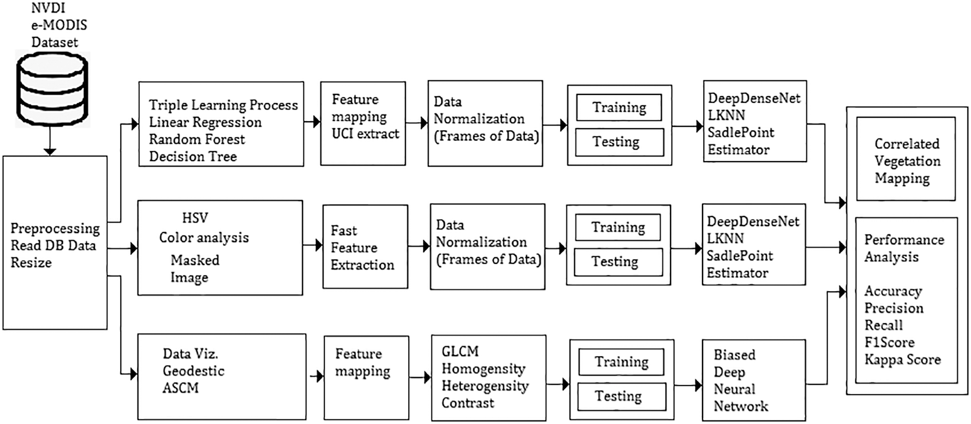
Figure 1: Cumulative architecture of proposed deep meta fusion model (DMFM)

Fig. 1 shows the system architecture of the proposed Deep Meta fusion model (DMFM) model. The proposed work considers the stacked operation of novel machine learning models for feature extraction and Deep learning Sense net for classification and mapping. Further, incorporating machine learning models within the system also improves the secure handling of data. The data originality is transformed and cannot disturb the uniqueness of the raw data.

3.1 Dataset Collection

The proposed model considers the USGS-Earth explorer data that provides access to the different global locations. It contains the geospatial data of earth’s imaginary collection from Unmanned aerial vehicles (UAV), IKONOS and National maps data accessed via interactive maps; it has geology, ecosystem, oceanic, water resources, and multi-media global access data. The proposed work considers the east European forest with few desert images collected for differentiation.

Fig. 2 shows the Sample test images of the USGS Earth Explorer NDVI eMODIS dataset, containing the vegetation and non-vegetation area covered globally. Despite various vegetation mapping techniques discussed in Section 2 and vegetation features discussed in Fig. 3, the proposed approach utilized (Colour) region-based mapping (CF), Unique feature-based mapping (UCF) and intensity-based mapping (IF).

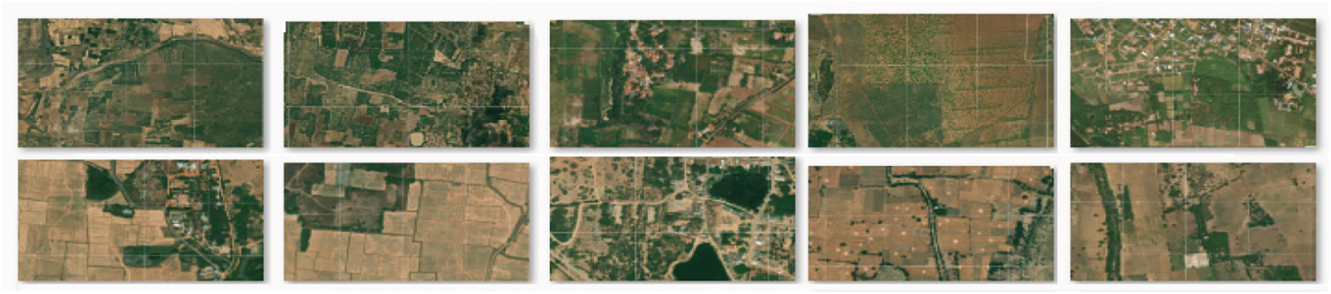
Figure 2: Sample test images of USGS earth explorer NDVI eMODIS dataset

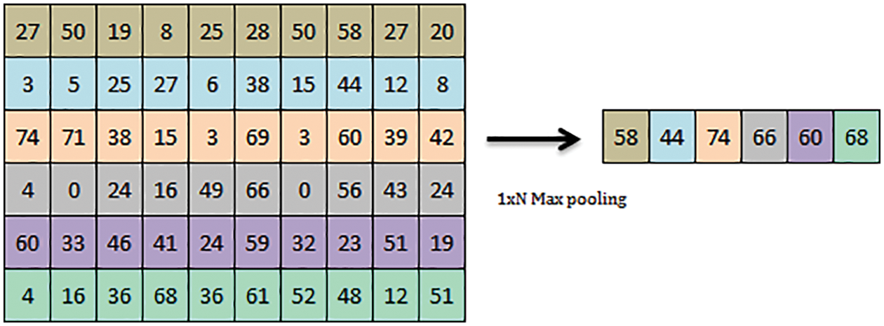
Figure 3: 1 x N maxpooling operation

3.2 Implementation Summary

The input images for the vegetation mapping process are collected from earth Explorer USGS. The input images are initially pre-processed by scaling the image size into constant since the data set images are different in scale. Colour masking and RGB segmentation are the first and foremost processes done with the pre-processing images. A unique colour masking process is done concerning the threshold of each channel of the images. The image consists of red, green and blue channels with a specific threshold ranging from 0 to 255. The requirement of vegetation colour lies at the channel, which is altered explicitly by the image masking tool. A slider is created based on the obtained minimum and maximum channel histogram threshold levels. A colour mask is projected concerning the channel minimum and maximum value and applied to the three channels equally. After the channel masking, the images are converted into constant projections by rotating colour space. A masked RGB image is created from 2D colour space pixels after the polygon application of slider value. These images are translated into the region of interest (ROI) location by using an image transformation matrix. The masked RGB image has a unique intensity pixel between the given space. Before the triple learning feature extraction, ionic components in the masked RGB images are extracted. The individual points are randomly distributed for the sample size. The sampling size used here is 100. The triple learning process for multi-feature extraction here uses logical regression, random forest regression and decision tree algorithms. A novel intermediate feature convergence technique is utilized in which the output of the loud linear regression is not required to grab the unique features of the input photos. On the other hand, the intermediate features of the logical regression random forest and decision tree algorithm for extracted and mapped. The proposed model is analyzed in two different steps; the first one extracts the unique features and formulates the feature-based analysis. The second one extracts the masked image for the region’s map using the colour masking technique and performs the region-based analysis. A detailed loop KNN that runs iteratively for the given features using a saddle for point estimator is evaluated. The resultant of lubrication and the saddle point estimator provides the masked features corresponding to the input images. A novel deep sense net technique is here assessed to analyze the region- and feature-based analysis in parallel. The modules of the proposed approach are categorized as three phases of operations to determine the novel method of vegetation mapping to the next level, comparing the existing frameworks [20,21].

4  Methodology

The proposed novel methodology is the fusion technique that incorporates the intermediate feature extraction using a Linear regression algorithm, Random Forest regression algorithm and Decision tree algorithm. Each machine learning algorithm has a unique way of representing the correlation score. The novelty of the proposed model is derived by extracting the intermediate values that act as unique point features of the input test and train images.

4.1 Preprocess

The pre-processing module consists of the following steps. Reading the input image Dataset from the specified location, we created a dataset of images collected from the USGS-eMODIS NDVI V6 dataset (Earth Explorer). We are segmenting the required area through the Colour Space mapping technique using the Colour Threshold application available with the image processing toolbox. The Colour Thresholder app lets you threshold colour images by manipulating the colour components of these images based on different colour spaces. Using this app, you can create a segmentation mask for a colour image. Colour Threshold opens the Colour Threshold app, enabling users to create a segmentation mask of a colour image based on exploring different colour spaces. We are initializing the length of the iterative loop and Sample size to be considered for each frame of analysis (100 samples of unique Pixels intensities). Display the input image, binary masked image, Colour Space mapped image etc.

4.2 Feature Study

The unique pixel intensities from the masked image are extracted using an individual command. Apply linear regression, Random Forest and Decision Tree algorithms separately to analyze the pixel intensities related to associated pixel intensities. For example, the vegetation area has a specific range of image intensities. The data split within the samples as Train intensity and Test intensity to transform the input unique pixel values into another form of intensity. These Correlated intensity values provide the exact vegetation area in the test image.

4.3 Significance of Machine Learning Models in Vegetation Feature Extraction

The feature extraction process is determined to grab the unique information in the form of numerical data from the given raw input, to secure the original data, and to allow the detection algorithm to make specific statistics and relativity between the data patterns.

•   It provides better results when applied to the raw data. The goal of the feature extraction process with the machine learning algorithm is discussed here, like Random Forest (RF), Decision Tree (DT) [22] and logistic regression (LR) to provide a multi-variation data pattern that provides unique identification of the input pattern [23].

•   The original image data from the dataset is transformed into pixels processing, and the originality of the image pixels is also secured.

•   In terms of existing feature extraction techniques, such as Principle component analysis (PCA) and Linear discriminant analysis (LDA) [24], the component axis maximizes until complete data coverage. Both the supervised and unsupervised methods lack user control over data separation complexity. Hence the automated process is applied for the Eigenvalues and Eigenspace vectors that are calculated.

•   The triple learning process developed here considers various aspects of intermediate features of RF, LR, and DT models to provide the top cumulative feature points.

4.4 Triple Learning Model (TLM)

The suggested approach uses a robust feature fusion technique, which combines three machine-learning techniques. The intermediate features are immediate values extracted after the colour masking process. Once the RGB colour space masking has been done, the triple-learning process maps the feature points together. In statistical analysis, linear regression considers the inputs linear and gathers the dependent variable from the given pattern. These values determine the relationship between the dependent variable with one or more independent variables. The generalized form of random forest regression is defined as.

Yilr=f(xilr,  β)+eilr  (1)

where Yilr→Dependent Variable , xilr→Independent Variable , β→Unknown parameter , eilr→Error terms

The Random Forest algorithm formulates the accumulation of numerous decisions. The forest depends on each independent decision of the trees. Higher the number of decisions, the denser the forest associated. Random forest is the summation of independent performance and is stated in (2) and (3).

Ynf=nfΣjεmax(nf)  (2)

Where nf→independent feature,  j→iterativenodes, Ynf→individual decision

In the same way, the random forest regression is denoted as the summation of total independent decision-making trees available to the total count of the trees.

Yirf=YnfT  (3)

T→Total number of trees

Similarly, the Decision tree algorithm is nothing but numerous intermediate decision makers that divides the large dataset into smaller couples of decision values. These decisions are regression results of the given input pattern at smaller spans. The decision-making process is the same as that of Eq. (2).

Feaife={Yilr, Yirf, Ynf } { j→Random Node} (4)

Feaife→intermediate feature extracted

The common features considered here are a colour feature, intensity feature, and unique attributes in the form of pixels are determined. Fig. 4 shows the proposed vegetation mapping framework using a multiple-feature extraction model with Deep Dense Net.

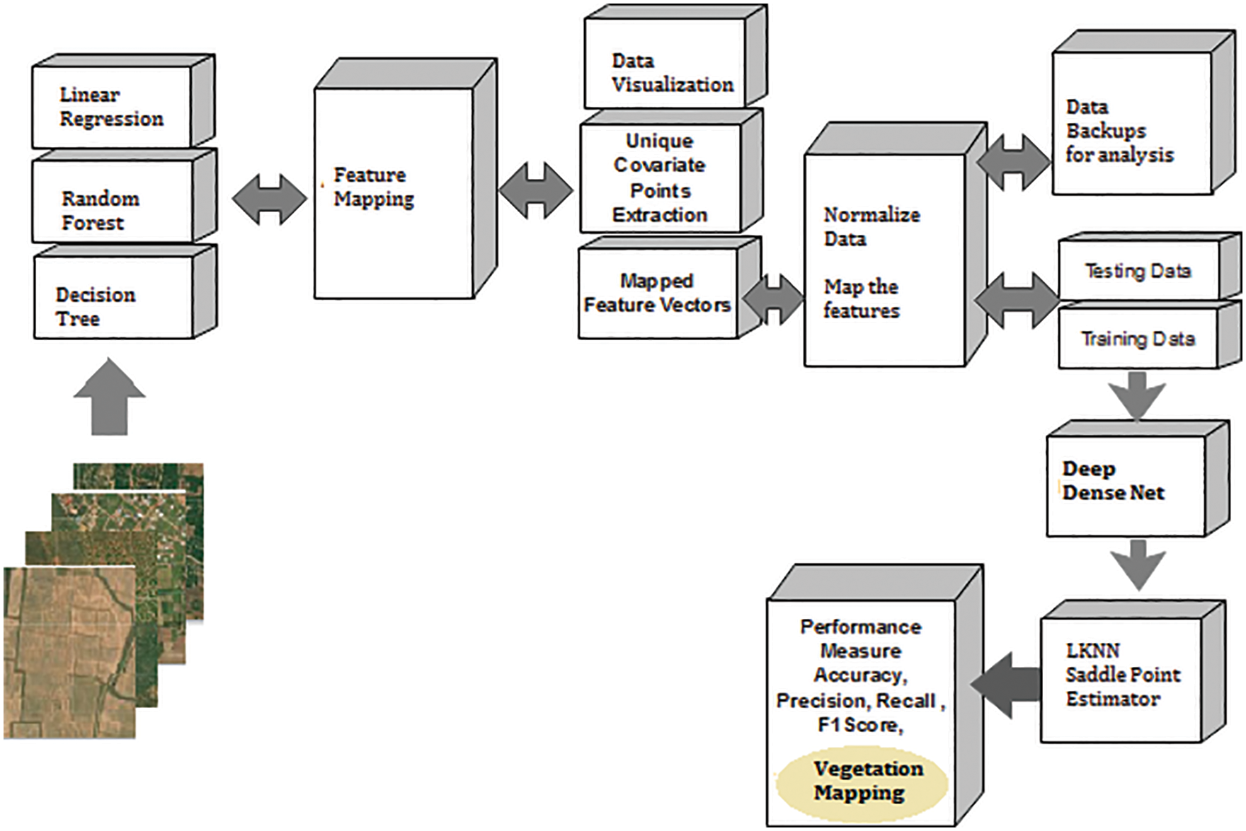
Figure 4: Unique covariate feature based vegetation mapping (UCF)

4.5 Novel Deep Sense-Net (NDSN)

Deep convolutional neural network act as the common deriving model for novelty in Deep Sense net. The convolution architecture comprises an image input layer of 100 × 100 ×1 and a 2D convolution layer of 1 × 10. The transfer function used in the Deep Sense net is Relu. The max-pooling of the 2D layer is evaluated, which consolidates the kernel to extract the maximum value from the patch. Max-pooling is used to convolute and downsample the long stream of the input layer. The max pooling operation minimizes the total scale of the convoluted input samples. Fig. 3 shows the max-pooling operation of 1 × 6 max pooling operation given as a sample. Further fully connected layers of scale 10 are repeated for 2 layers, followed by fully connected layer 1 is structured. The softmax layer is used to normalize the values to round off the nearest equivalent for flexible classification. The final classification layer formulates the matched pattern of vegetation images for further mapping the regions.

The convolution neural network is trained with a stochastic gradient descent optimizer (SGD). The classification process is performed with two modes of operation, feature-based analysis and region-based analysis. SGD optimizer is used for complete training of masked images in the region-based analysis and features mapped study in the second method.

4.6 Stochastic Gradient Descent Optimizer (SGD)

The feature input values fetched from the triple learning process are further optimized with a stochastic gradient Descent process which is an attractive method for optimizing the input values for the objective function. These optimizers must tune the difference and sub deference input values adaptively. The feature values are not exactly matching with the training values. To make a matching score, these values need to be differentiated by tuning the values with the tolerance. Gradient Descent optimizers are helpful for randomly making the subset of the data required to prevent it from being used for dimensionality reduction. The stochastic approximation method is based on the Robbins-Monroe algorithm.

Q(w)=1n∑i=1nQi(w)  (5)

w→Parameter that minimizes Q(w) 

Qi(w)→Each equivated function is associated with ith variable

w=w−μΔQi(w)

μ→learning rate of the algorithm

In stochastic gradient descent, the true gradient of Q(w) is approximated by a gradient of different samples. As the Novel algorithm sweeps through the full span of the training set, it performs the above update for each training example. Several passes can be made over the training set until the algorithm converges. If this is done, the data can be shuffled for each pass to prevent cycles.

4.7 Looped K-Nearest Neighbor

The K-nearest neighbour algorithm is used for non-parametric classification and regression needs. The closest training sample is compared with the given test sample in which the object related to the training sample is identified by differentiation. At K, the nearest neighbour algorithm defines the Kth nearest value applicable to the training data for the complete iterations.

4.8 Saddle Point Estimator

From the iterative analysis with Deep Sensenet with two modes, feature-based analysis and region-based analysis, the complete correlation process runs to the maximum of looped k-nearest neighbour (KNN). The saddle point is the maximum occurring threshold in the complete iteration process. The saddle points help to reach the nearest match of the image features with the training features that maps the vegetation area. The saddle point is defined as the maximum threshold value frequently occurring within the looped k-nearest neighbour (KNN). The saddle point estimator formulates the threshold value that frequently occurs from the n iterations of the looped k-nearest neighbour (KNN). The match score determines the exactness of the vegetation pattern match with the training images.

4.9 Unique Covariate Feature Based Vegetation Mapping (UCF)

The unique covariate points are extracted from LR, DT, and RF collaborated triple feature learning (TFL) process. The intermediate features are fetched to extract the unique covariate pixel features (UCF) (Fig. 4).

These points are nothing but the normalized feature vectors created to test the proposed model. The data split up is implemented using test data and fetched into Deep Densenet for classification. Further, the Looped KNN is the iterative loop of the nearest point calculator required to correlate with the relative match score. The saddle point estimator is the final suggestion maker that considers the decision made by the proposed different parametric results and further estimates the final decision.

4.10 Colour Feature or Region Based Vegetation Mapping (CF)

Fig. 5 shows the Colour feature-based segmentation process called the region-based segmentation model. Here colour threshold app is utilized to vary the colour space to the required level, and the region is extracted. The region extracted is masked with the background elimination scheme and further, using mean square error (MSER) feature points, the combined feature mapping is done as shown in Section 5. A hexagon is a 3D representation of the HSV colour space, where the central vertical axis represents the intensity of the pixels. Here, Hue is defined by the ranges [0, 2S], Red axis with red at angle 0, green at 2S/3, blue at 4S/3 and red again at 2S. Overload is the depth of the colour, and it is changed from the axis with a value between 0 at the center to 1 at the outer surface.

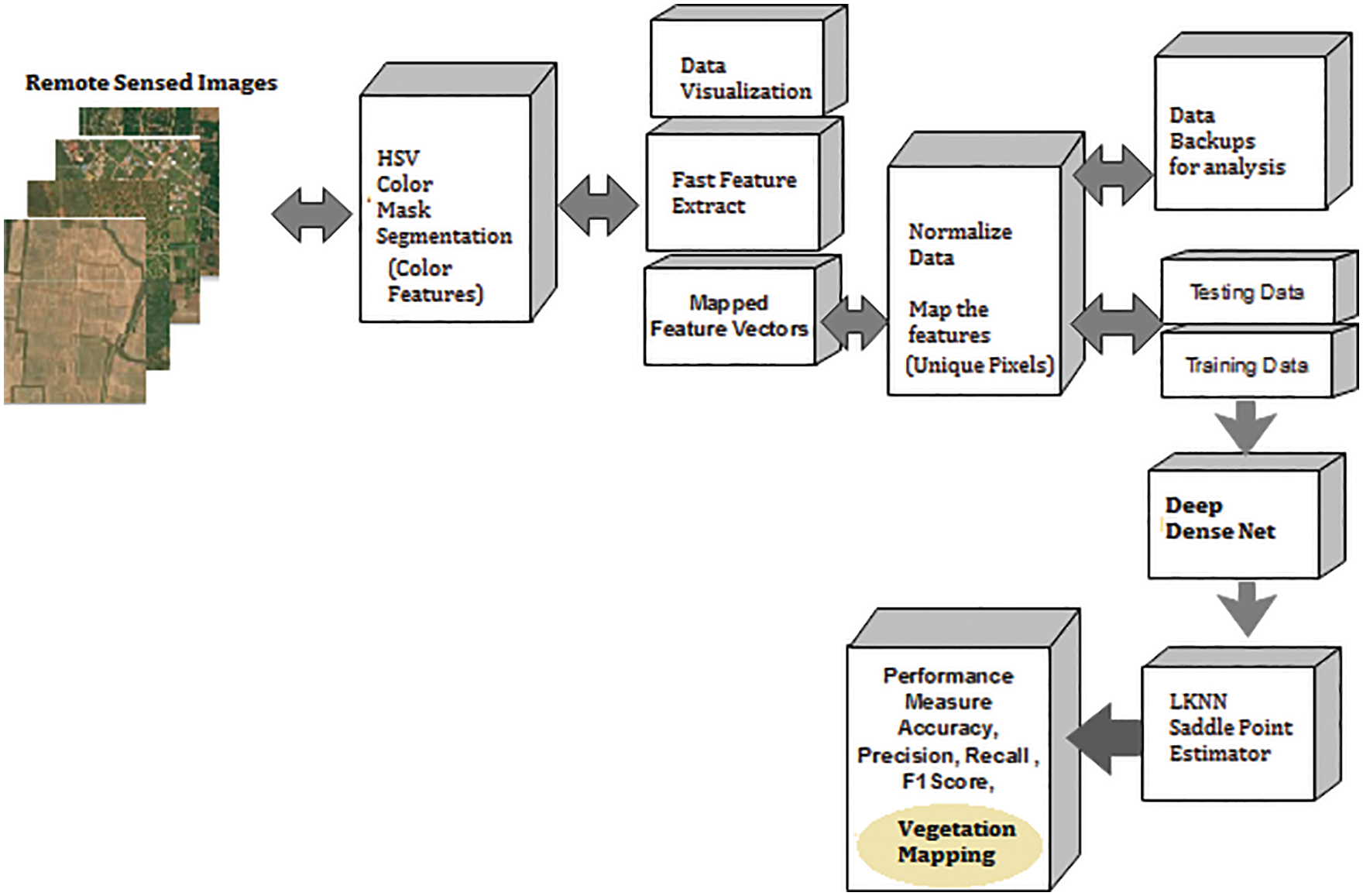
Figure 5: Colour feature or region based vegetation mapping (CF)

4.11 Intensity Feature-Based Vegetation Mapping (IF)

Fig. 6 shows the proposed novel intensity-based vegetation mapping model using the Geodetic automated snake convergence model (ASCM) model with gray level co-occurrence matrix (GLCM) for texture feature extractions. Parameters such as Heterogeneity, homogeneity and Contrast are evaluated.

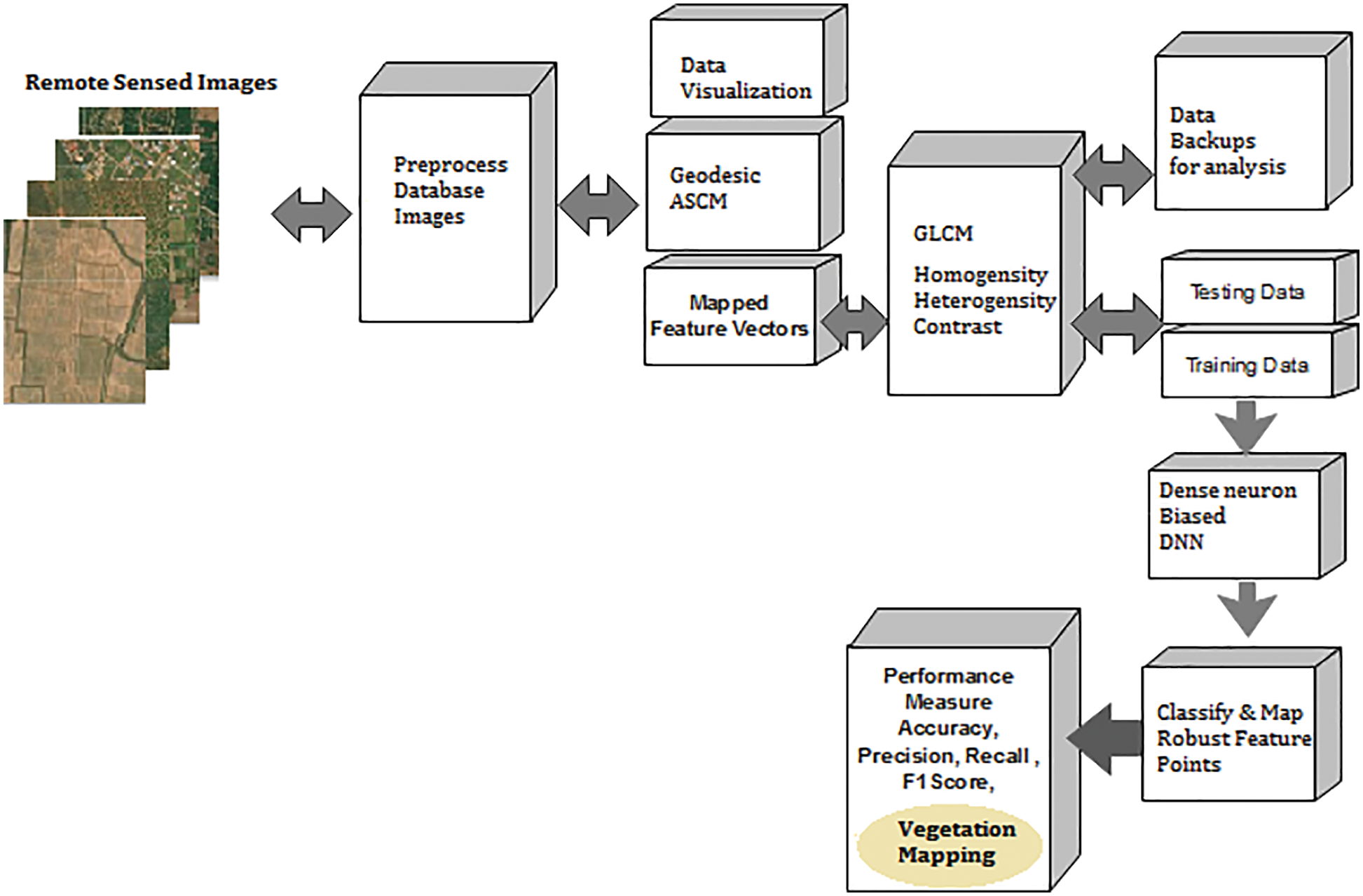
Figure 6: Proposed novel intensity-based vegetation mapping model

4.12 Automated Snake Convergence Model (ASCM)

Mathematical dynamic shape (GAC) is a form model that changes the Euclidean smooth bend by changing the bend’s focus in opposite directions. The focus moves at a rate proportionate to the shape of the picture’s district. The mathematical progression of the angle and the acknowledgement of things are utilized to portray forms. Mathematical stream envelops inside and outside mathematical measures in the area of interest. During the time spent recognizing things in an image, a mathematical substitution for snakes is used. These form models depend vigorously on fair and square set works that determine the picture’s special locales for division. GLCM gray covariance matrix is one of the robust techniques for extracting the features present in the test images. Further, the images estimate the probability that distant sets of pixel values will occur in the image. This calculation is known as GLCM. The framework characterizes the likelihood of joining two pixels with values I and j with distance d and as a precise direction.

4.13 Performance Metrics

Kappa Score-Cohen’s kappa is the statistical evaluation technique used to represent the amount of system accuracy and reliability in statistical calculations. It is identified between two recommended results to evaluate accuracy. The Kappa score is calculated by the formula below.

k=p0−pe1−pe (6)

where P0 is a relatively observed agreement, Pe defines the hypothetical probability of chance agreement. A value nearer to 1.0 represents a high agreement.

5  Results and Discussions

RGB masking is done, and the equivalent feature component after the Triple learning process is shown in Fig. 7. The features of single frame 1 × 100 are displayed with the results above, which determines the pixel intensity of the given test image.

Figure 7: RGB colour masking, feature component extraction

Fig. 8 shows the various stages of Vegetation mapping Region segmentation, Pseudo colour mapping of segmented regions and Region extraction through the ASCM model is shown. Finalize the combined feature mapped into the complete area available for vegetation using Markers Evaluation.

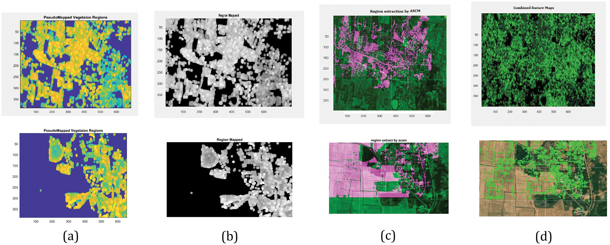
Figure 8: Simulated results of various stages of vegetation mapping (a) Pseudocode mapped vegetation region, (b) Region mapped, (c) Region extracted by ASCM, (d) Combined feature mapped

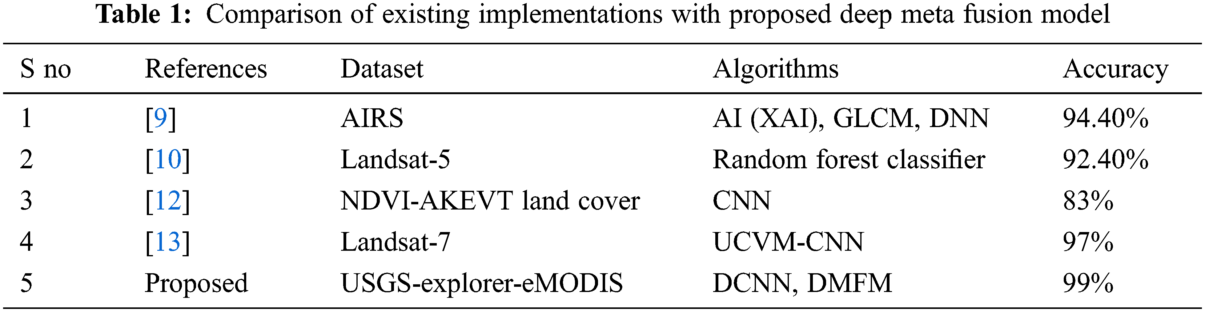
Table 1 shows the comparison of similar frameworks implemented with different datasets of vegetation mapping [9]. Using the AIRS dataset, an Explainable AI architecture is discussed. The Deep neural network model, combined with GLCM-based feature extraction study statistical measures, implies classifying the vegetation mapping with an accuracy of 94.4%. This existing implementation is a basic ideology for utilizing machine learning algorithms in the vegetation mapping system [12]. Discuss the NDVI-AKEVT Land Cover dataset with Convolutional Neural network (CNN) architecture, the accuracy of 83% is achieved [13]. Discuss the Landsat-7 dataset using the unsupervised classification method of Vegetation mapping (UCVM) with CNN is performed. An accuracy of 97% is achieved with the presented method. Comparatively, the proposed method of the Deep-meta fusion model combines the achieved accuracy of 99%. With limited iterations in the looped KNN, the classification process is done. The utilization of CNN architecture increases GPU engagement and system overhead if more complex data is provided. GLCM considers the grayscale features only. On the other hand, vegetation exploration is not only considered by the texture but also important colour features. The comprehensive data with labels are not available for all dataset, and real-time dataset need to be analyzed. Hence random forest algorithm explained in [10, 25–30] needs to be improved. The proposed DMFM considers all these constraints and details the features, classification and computation time.

Kappa Coefficient of Existing Model and Proposed DMFM Technique Table 2 shows the comparison chart of existing and proposed Kappa Coefficient values with existing and proposed DMFM model, calculated by kappa = (total accuracy-random accuracy)/(1-random accuracy). Lee et al., discussed the NDVI vegetation mapping framework and achieved KC = 0.8. Shaik et al., in terms of detecting the Wildfire framework using a vegetation mapping system, achieved the KC = 0.79 with PRISMA data. Weil et al., utilized a woody vegetation framework with UAV images and achieved the KC = 0.82. Despite a damaged vegetation mapping system, Haque et al., using Sentinel-2 data, achieved the KC = 0.1. The proposed DMDF system achieved the KC = 0.9.

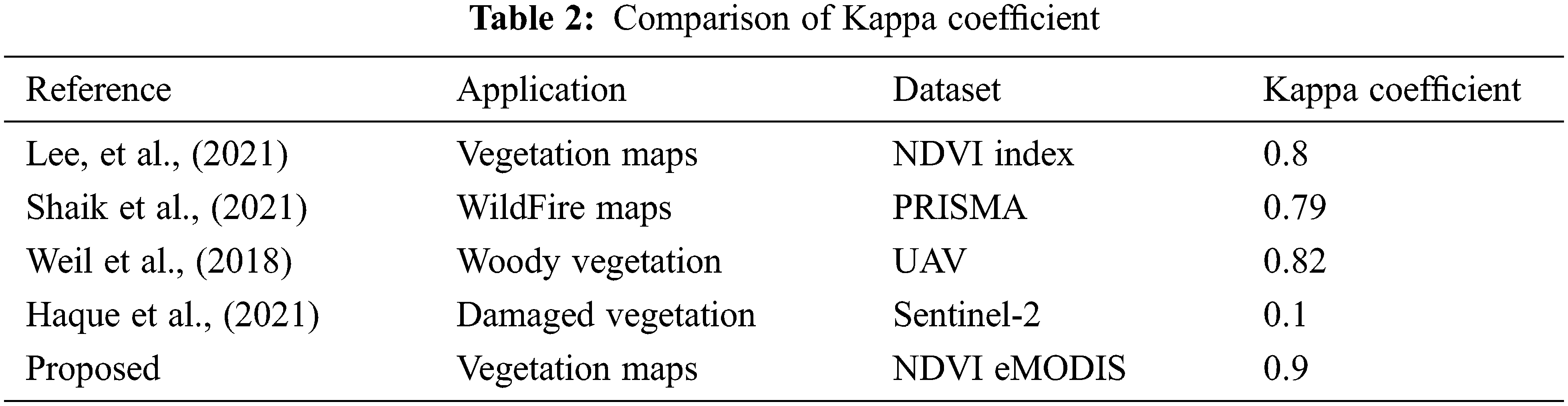
Table 3 shows the comparison of various performance metrics obtained from three levels of implementations done with the proposed work. The metrics include accuracy, Precision, Recall, F1Score, Specificity, sensitivity, etc. The table shows the justification of each method that is helpful in finding the vegetation maps accurately. The UCF-based technique achieved 98%, the CF method derived 96%, and the IF method achieved 97% accuracy (see Fig. 9). The final accuracy of 99% is obtained using the DMFM method.

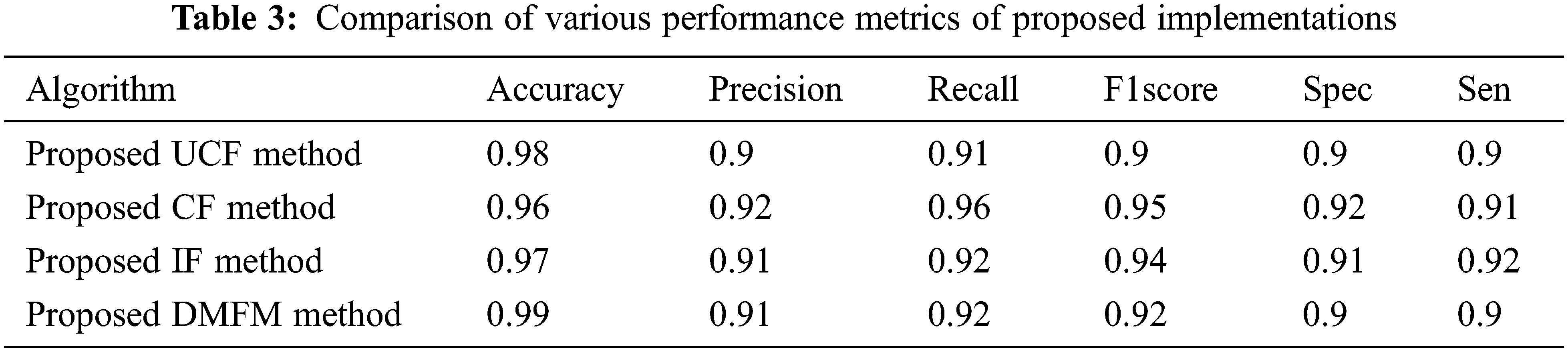
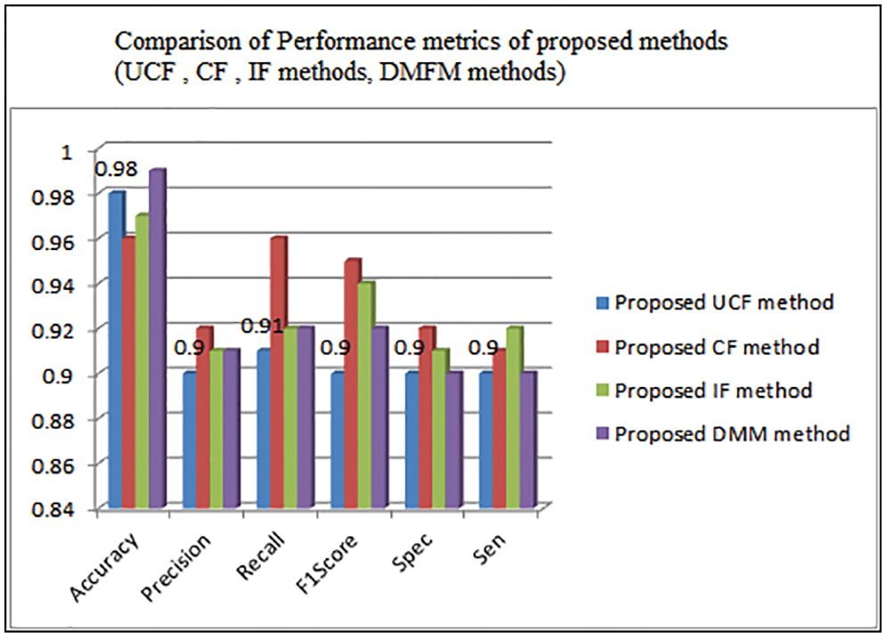
Figure 9: Comparison of performance metrics of UCF,CF,IF,DMFM methods

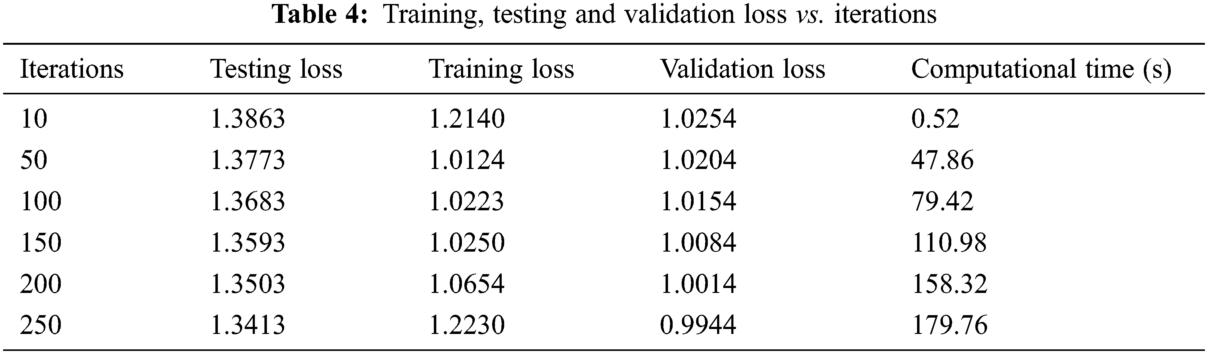
Fig. 10 and Table 4 shows the Training, Testing and Validation Loss to the number of iterations the test is being conducted. The average Training loss is 1.0937, and the average testing loss is 1.3638, the average validation loss is 1.0909 etc. The proposed system achieves less training, testing and validation loss as the number of iterations increases.

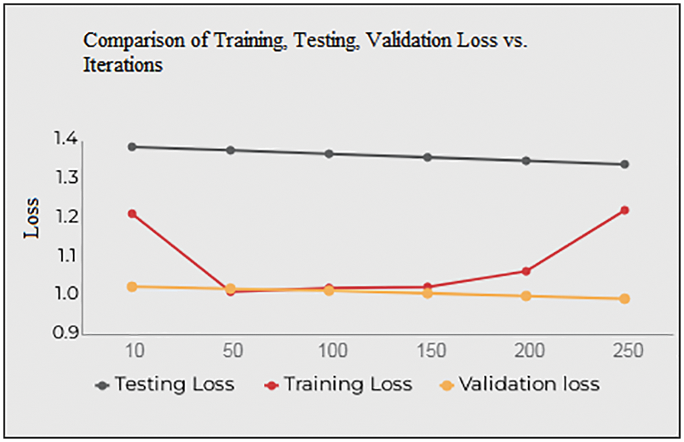
Figure 10: Training, testing, validation loss vs. iterations

6  Conclusion

The novel implementation of vegetation mapping is evaluated here. Vegetation mapping is important to maintain the ecosystem and formulate the vegetation areas’ healthiness. Mapping the vegetation patterns using remote sensing images is discussed here. The presented model considers the Earth Explorer-USGS-eMODIS-NDVI V6 dataset that contains the overall images of earth vegetation areas in high resolution. The novel Deep Meta fusion model (DMFM) is implemented here to create a robust architecture that extracts the features of the input images through a feature- and region-based approach. Based on the evaluated features, Deep Sensenet architecture performs a higher accuracy of 99% for the static data given from the USGS dataset. The system developed here is a lightweight architecture to map global data effectively. The accuracy of the proposed model is 99%, precision is 91%, Recall is 92%, F1Score is 92% precision, Specificity is 90% specificity, 90% etc. The looped KNN presented here is dynamic that adaptively adjusts the weights of the threshold and length of the loop depending on the complexity of the input images. Validation of similar pattern structure to training images and considering UCF, IF, and CF parameters further help to make robust decisions. It adds strength to the decision rule. Various parametric measured even the Kappa coefficient is achieved around 0.9, nearer to Score 1, which is the positive highlight of the proposed work. Further, the proposed model is extended by utilizing the categorized vegetation data using YoLo frameworks.

Acknowledgement: The authors would like to thank the Department of Computer Science and Engineering, Saveetha School of Engineering, SIMATS, for their support till the completion of this project.

Funding Statement: The authors received no specific funding for this study.

Conflicts of Interest: The authors declare they have no conflicts of interest to report regarding the present study.

References

1. R. Xu, S. Zhao and Y. Ke, “A simple phenology-based vegetation index for mapping invasive spartina alterniflora using google earth engine,” IEEE Journal of Selected Topics in Applied Earth Observations and Remote Sensing, vol. 14, no. 1, pp. 190–201, 2021. [Google Scholar]
2. Y. Li, J. Shi, Q. Liu, Y. Dou and T. Zhang, “The development of microwave vegetation indices from windsat data,” IEEE Journal of Selected Topics in Applied Earth Observations and Remote Sensing, vol. 8, no. 9, pp. 4379–4395, 2015. [Google Scholar]
3. Y. Huang, J. P. Walker, Y. Gao, X. Wu and A. Monerris, “Estimation of vegetation water content from the radar vegetation index at L-Band,” IEEE Transactions on Geoscience and Remote Sensing, vol. 54, no. 2, pp. 981–989, 2016. [Google Scholar]
4. B. Meng, Y. Zhang, Z. Yang, Y. Lv, J. Chen et al., “Mapping grassland classes using unmanned aerial vehicle and MODIS NDVI data for temperate grassland in inner Mongolia, China,” Remote Sensing, vol. 14, no. 9, pp. 1–17, 2022. [Google Scholar]
5. A. L. C. Ottoni and M. S. Novo, “A deep learning approach to vegetation images recognition in buildings: A hyperparameter tuning case study,” Latin America Transactions, vol. 19, no. 12, pp. 2062–2070, 2021. [Google Scholar]
6. T. Wu, J. Luo, L. Gao, Y. Sun, Y. Yang et al., “Geoparcel-based spatial prediction method for grassland fractional vegetation cover mapping,” IEEE Journal of Selected Topics in Applied Earth Observations and Remote Sensing, vol. 14, no. 1, pp. 9241–9253, 2021. [Google Scholar]
7. T. D. Mushore, O. Mutanga and J. Odindi, “Determining the influence of long term urban growth on surface urban heat islands using local climate zones and intensity analysis techniques,” Remote Sensing, vol. 14, no. 9, pp. 1–22, 2022. [Google Scholar]
8. C. Pelletier, I. Webb and F. Petitjean, “Temporal convolutional neural network for the classification of satellite image time series,” Remote Sensing, vol. 11, no. 1, pp. 523–527, 2019. [Google Scholar]
9. A. Abdollahi and B. Pradhan, “Urban vegetation mapping from aerial imagery using explainable AI (XAI),” Sensors, vol. 21, no. 14, pp. 1–16, 2021. [Google Scholar]
10. M. S. Beon, K. H. Cho, H. O. Kim, H. K. Oh and J. C. Jeong, “Mapping of vegetation using multi-temporal downscaled satellite images of a reclaimed area in Saemangeum, Republic of Korea,” Remote Sensing, vol. 9, no. 272, pp. 1–17, 2017. [Google Scholar]
11. M. Campos-Taberner, F. J. García-Haro and B. Martínez, “Understanding deep learning in land use classification based on Sentinel-2 time series,” Scientific Reports, vol. 10, no. 1, pp. 17188, 2020. [Google Scholar] [PubMed]
12. B. Ayhan, C. Kwan, B. Budavari, L. Kwan, Y. Lu et al., “Vegetation detection using deep learning and conventional methods,” Remote Sensing, vol. 12, no. 15, pp. 2502, 2020. [Google Scholar]
13. Z. J. Langford, J. Kumar, F. M. Hoffman, A. L. Breen and C. M. Iversen, “Arctic vegetation mapping using unsupervised training datasets and convolutional neural networks,” Remote Sensing, vol. 11, no. 69, pp. 1–23, 2019. [Google Scholar]
14. B. Xie, C. Cao, M. Xu, X. Yang, R. S. Duerler et al., “Improved forest canopy closure estimation using multi-spectral satellite imagery within google earth engine,” Remote Sensing, vol. 14, no. 9, pp. 1–15, 2022. [Google Scholar]
15. L. Jiang, Y. Yang and S. Shang, “Remote sensing-based assessment of the water-use efficiency of maize over a large, arid, regional irrigation district,” Remote Sensing, vol. 14, no. 9, pp. 1–16, 2022. [Google Scholar]
16. S. Vijayalakshmi and G. Dilip, “A newest data set analysis for remote sensing applications,” Journal of Advanced Research in Dynamical & Control Systems”, vol. 11, no. 4, pp. 1064–1067, 2019. [Google Scholar]
17. J., Xu, G. Feng, B. Fan, W. Yan, T. Zhao et al., “Landcover classification of satellite images based on an adaptive interval fuzzy c-means algorithm coupled with spatial information,” International Journal of Remote Sensing, vol. 41, no. 6, pp. 2189–2208, 2020. [Google Scholar]
18. S. Vijayalakshmi and M. Kumar, “Accuracy prediction of vegetation area from satellite images using convolutional neural networks,” Turkish Journal of Physiotherapy and Rehabilitation, vol. 32, no. 3, pp. 1730–1741, 2022. [Google Scholar]
19. S. Vijayalakshmi, S. Magesh Kumar and M. Arun, “A study of various classification techniques used for very high-resolution remote sensing [VHRRS] images,” in Proc. Materials Today: Proc., Chennai, India, vol. 37, no. 2, pp. 2947–2951, 2021. [Google Scholar]
20. J. Zhou, Y. Huang and B. Yu, “Mapping vegetation-covered urban surfaces using seeded region growing in visible-NIR air photos,” IEEE Journal of Selected Topics in Applied Earth Observations and Remote Sensing, vol. 8, no. 5, pp. 2212–2221, 2015. [Google Scholar]
21. W. Yang and W. Qi, “Spatial-temporal dynamic monitoring of vegetation recovery after the wenchuan earthquake,” IEEE Journal of Selected Topics in Applied Earth Observations and Remote Sensing, vol. 10, no. 3, pp. 868–876, 2017. [Google Scholar]
22. K. L. Bakos and P. Gamba, “Hierarchical hybrid decision tree fusion of multiple hyperspectral data processing chains,” IEEE Transactions on Geoscience and Remote Sensing, vol. 49, no. 1, pp. 388–394, 2011. [Google Scholar]
23. A. A. Kzar, H. S. Abdulbaqi, H. S. Lim Ali, A. Al-Zuky and M. Z. Mat Jafri, “Using of linear regression with THEOS imagery for TSS mapping in Penang Strait Malaysia,” European Journal of Research, vol. 5, no. 1, pp. 26–39, 2020. [Google Scholar]
24. E. Hidayat, N. A. Fajrian, A. K. Muda, C. Y. Huoy and S. Ahmad, “A comparative study of feature extraction using PCA and LDA for face recognition,” in Proc. 2011 7th Int. Conf. on Information Assurance and Security (IAS), New York, USA, pp. 354–359, 2011. [Google Scholar]
25. T. Rajendran, P. Valsalan, J. Amutharaj, M. Jennifer, S. Rinesh et al., “Hyperspectral image classification model using squeeze and excitation network with deep learning,” Computational Intelligence and Neuroscience, vol. 2022, no. 9430779, pp. 01–09, 2022. [Google Scholar]
26. M. B. Sudan, T. Anitha, A. Murugesan, R. C. P. Latha, A. Vijay et al., “Weather forecasting and prediction using hybrid C5.0 machine learning algorithm,” International Journal of Communication Systems, vol. 34, no. 10, pp. e4805, 2021. [Google Scholar]
27. C. Narmatha and P. M. Surendra, “A review on prostate cancer detection using deep learning techniques,” Journal of Computational Science and Intelligent Technologies, vol. 1, no. 2, pp. 26–33, 2020. [Google Scholar]
28. S. Manimurugan, “Classification of Alzheimer's disease from MRI images using CNN based pre-trained VGG-19 model,” Journal of Computational Science and Intelligent Technologies, vol. 1, no. 2, pp. 34–41, 2020. [Google Scholar]
29. R. S. Alharbi,H. A. Alsaadi, S. Manimurugan,T. Anitha and M. Dejene, “Multiclass classification for detection of COVID-19 infection in chest X-Rays using CNN,” Computational Intelligence and Neuroscience, vol. 2022, no. 3289809, pp. 1–11, 2022. [Google Scholar]
30. M. Shanmuganathan, S. Almutairi, M. M. Aborokbah, S. Ganesan and V. Ramachandran, “Review of advanced computational approaches on multiple sclerosis segmentation and classification,” IET Signal Processing, vol. 14, no. 6, pp. 333–341, 2020. [Google Scholar]
Cite This Article
Copyright © 2023 The Author(s). Published by Tech Science Press.
This work is licensed under a Creative Commons Attribution 4.0 International License , which permits unrestricted use, distribution, and reproduction in any medium, provided the original work is properly cited.
Downloads
Citation Tools