A Novel Deep Learning Representation for Industrial Control System Data

1  Introduction

With the continuous development of cloud computing and industrial Internet, malicious attacks against industrial control systems are also constantly emerging. Therefore, it is becoming more and more important to determine in a timely manner whether an industrial control system is attacked based on the features of its operating states [1,2]. Machine learning technology provides a feasible, efficient, effective potential solution for in-depth analyses of the operating state data of industrial control systems. It can help system administrators obtain the risk information of a system through the analysis of a large amount of data, so as to take corresponding appropriate countermeasures and greatly improve system security [3,4]. In addition, in the practical application of industrial control systems, many complex features of the system’s operating states collected by its administrators usually contain numerous communication network data features extracted from industrial sensors, industrial actuators, industrial transmitters, and industrial controllers. Therefore, the development of high-performance and high-accuracy machine learning algorithms to analyze the operating state data of industrial control systems has become one of the hottest research topics in the field of information security of industrial control systems.

The success of machine learning algorithms largely depends on feature selection and data representation [5,6]. However, it is challenging to represent and model industrial control data due to their high dimension, noise, heterogeneity, sparsity, incompleteness, random errors, and systematic deviations. In particular, it is a very important and difficult task to achieve effective dimensionality reduction for high-dimensional industrial control datasets in the presence of inevitable noise. The main purpose of dimensionality reduction is to eliminate redundant data in the original datasets and represent them in a more efficient and economical way.

At present, supervised feature selection strategies are the most popular method. In current practice, the feature selection process of industrial control datasets mainly depends on domain experts to specify patterns (i.e., learning tasks and learning objectives) and reasonably extract the corresponding features [7]. Several other supervised feature selection algorithms, such as linear discriminant analysis [8], compressive sensing [9], and the hidden Markov model [10], have been developed and obtained good application effects in different fields. Although the above-mentioned supervised methods are suitable in certain cases, their actual effects will largely depend on the prior information of domain knowledge and data structure, which is not entirely available in every case, and the supervised definition scale of feature space is very poor. Consequently, some new patterns or hidden features in the original data are always missed, which eventually makes such supervised feature selection methods difficult to be well popularized.

To avoid the shortcomings of supervised methods, research on unsupervised feature selection methods has attracted extensive attention. As one of the most representative conventional unsupervised methods, principal component analysis (PCA) [11] ignores the important nonlinear relationship between features of high-dimensional data and only makes a linear low-dimensional representation, which leads to limited applications. Recently, deep-learning-based unsupervised feature selection methods have seen significant development; their core idea is to attempt to overcome the limitations of the supervised feature space definition by automatically identifying patterns and dependencies in data, so as to learn compact and general representations, making it easier to automatically extract useful information when constructing classifiers or other predictors [12,13]. In particular, autoencoder-based unsupervised feature selection methods have been widely used in many fields due to their ability to display and learn compact representations. As a type of special unsupervised neural network framework, an autoencoder consists of two parts: 1) the encoder realizes the dimensionality reduction of high-dimensional features; 2) and the decoder reconverts the low-dimensional representations [14]. Finally, the encoded and decoded network parameters are trained by reconstructing the errors between input and output. However, to our knowledge, the use of autoencoder-based feature selection techniques that enable the original data to form a low-dimensional representation with abstract features for subsequent efficient data processing and analysis have not been well popularized in the field of industrial control.

In practice, the multi-sensor features of industrial control data are usually strongly correlated, which is ignored in the full connection layer of the conventional autoencoder. On the other hand, due to the strong sensor noise in industrial control systems, autoencoders are facing a new development challenge to further realize better low-dimensional representations and information recovery of the original data.

Based on the above discussions, in this paper, a novel industrial control data expression model framework is presented; its specific scheme is outlined in Fig. 1. First, a convolutional neural network with a powerful ability for feature selection is employed to replace the full connection layer of traditional autoencoders to further mine the correlations between data. Then, to solve the noise problem, a deep neural network composed of denoising autoencoders is used to process the industrial control data in an unsupervised way, and capture the stable structure and regular patterns of the data. Subsequently, these patterns are combined to form a deep industrial control representation that does not require any manpower or expert experience for additional feature selection tasks and can be easily applied to different prediction applications, as well as supervised and unsupervised learning. Finally, the effectiveness and superiority of the proposed representation method are verified based on an operating state experiment of a large-scale SWaT water treatment industrial control system and a bearing dataset. We input the low-dimensional features captured by the proposed novel autoencoders into the machine learning model and demonstrate the reliability of the autoencoder model for deep industrial control safety state data. To summarize, our major contributions are as follows:

A)   We propose a novel autoencoder model for large-scale industrial control system (ICS) data. The deep industrial feature learning model (DIFL) can better obtain higher-order features while preserving the original data information.

B)   This study contributes to the effective analysis of large-scale ICS data, which promotes the stable operation of ICS.

C)   We showcase how well our proposed model performs in the ICS based on two case studies.

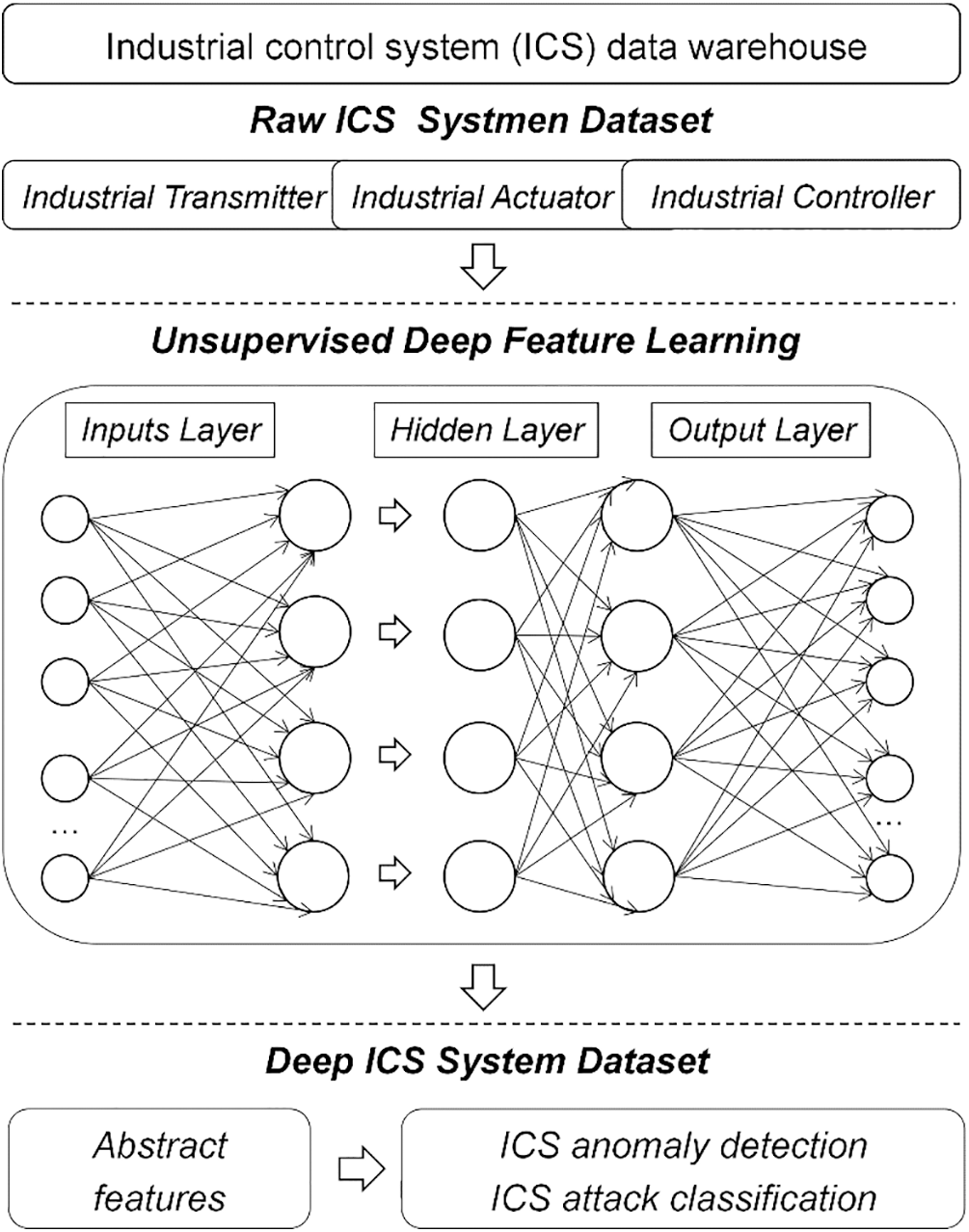
Figure 1: A novel industrial control data expression model framework

The remainder of this paper is organized as follows. Section 2 elaborates upon our proposed method. Section 3 verifies the effectiveness and superiority of the proposed method through a series of comparative experiments. The major conclusions are made in the Section 4.

2  Methods

In this section, we introduce our deep feature learning framework for ICS data in three parts (Fig. 2). In the preprocessing part, we regularized the ICS data by data standardization and data balance. In the feature learning part, the high-dimensions ICS data were transformed into low-dimensions using our DIFL framework efficiently. In the classification part, two normal machine learning methods were applied to industrial control risk status assessment using our low-dimensions features.

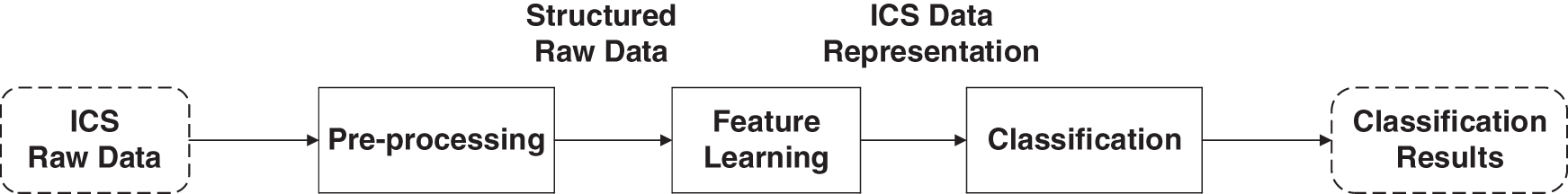
Figure 2: Deep feature learning framework

2.1 Preprocessing

ICS data With the development of Industry 4.0, more and more industrial data are collected through different sensors. These features in ICS data have different dimensions and orders of magnitude, and features have effects on the operating state of the system. In ICS datasets, there is a serious imbalance between the amounts of normal and attacked states [15]. Therefore, data preprocessing is necessary.

2.1.1 Data Standardization

Data standardization refers to the conversion of data into dimensionless evaluation indicators, thereby unifying the order of magnitude of the data. Data standardization can balance the impact of various characteristics on the operating state of the system and lay the foundation for subsequent data analysis.

We use the z-score standard deviation standardization method to preprocess the data, namely x=(x−avg)/σ) , where (x) is the data to be processed, (avg) is the average value of the data, and ( σ ) is the standardized variance.

2.1.2 Data Balance

To address the impact of data balance on the classification results, this paper adopts the Borderline SMOTE oversampling method to delete the normal state data. This method synthesizes new samples for a small part of the samples on the data boundary and then improves the distribution of the overall sample.

For the entire sampling process, we divide the minority samples in the data samples into three categories: safe samples, danger samples, and noise samples (see Fig. 3. below for details).

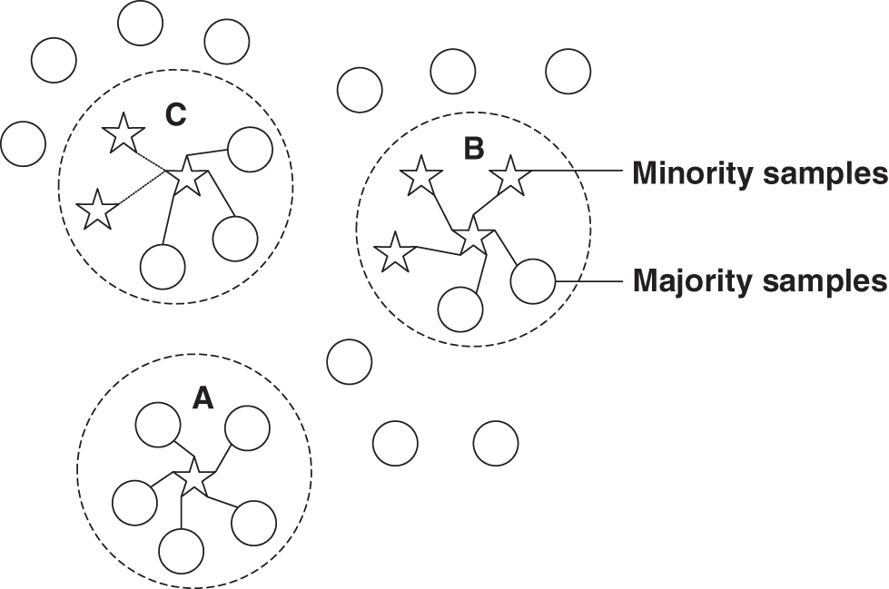
Figure 3: Classification of samples. Point B represents when more than half of the samples around the sample are minority samples, which is a safe sample. Point C when more than half of the samples around the sample are majority samples, which is a danger sample. Point A represents when there are no minority samples around the sample, which is a noise sample.)

2.2 Feature Learning

2.2.1 Autoencoder

An autoencoder is a neural network that uses a back-propagation algorithm to make the output value equal to the input value. It first compresses the input into a latent space representation and then reconstructs the output through this representation. The autoencoder consists of two parts:

Encoder: This part compresses the input into a latent space representation.

Decoder: This part reconstructs the input from the latent space representation.

The mapping of the autoencoder consists of two processes: encoding and decoding, where the encoding process compresses the input high-dimensional data into low-dimensional data, and the decoding process reverts the low-dimensional data to high-dimensional data.

The function of the autoencoder is to perform dimensionality reduction operations, transform the original data into low-dimensional data through the encoding process, then analyze the low-dimensional data and convert the analysis results into high-dimensional data through the decoding process. High-dimensional processing effects are achieved through low-dimensional processing methods.

The purpose of this network is to reconstruct its input so that its hidden layers learn a good representation of that input. If the input is exactly equal to the output, the network is meaningless. Therefore, some constraints need to be imposed on the autoencoder so that it can only approximately replicate the raw data. These constraints force the model to consider which parts of the input data need to be replicated preferentially, so it tends to learn useful properties of the data. There are generally two constraints:

1.    Making the dimension of the hidden layer smaller than that of the input is called being under-complete. The encoder reduces the dimension of the data, and the decoder restores the data (similar to PCA). If there are fewer hidden nodes than visible nodes (input, output), due to the forced dimensionality reduction, the autoencoder will automatically learn the features of the training samples (the most varied and informative dimension).

2.    Making the dimension of the hidden layer larger than the dimension of the input data is called being over complete. If the number of hidden nodes is too large, the autoencoder may learn an “identity function,” which directly copies the input as the output. Therefore, other constraints need to be added, such as regularization and sparsity.

The structure of the autoencoder is shown in Fig. 4.

Figure 4: The structure of the autoencoder

2.2.2 Deep Industrial Feature Learning

To solve the problem that the data collected by ICS sensors often contain significant noise, this paper uses an improved denoising autoencoder (DAE), named DIFL, to extract the features of the original data. DIFL is based on the traditional AE, adding noise data to the input data to form a complex sample containing noise, and then reconstructing the characteristic data. When training, we input the noise-added data into the input layer, and the reconstruction target of the autoencoder (AE) is still the data without noise. Through this training method, the effective essential characteristics of the data can be obtained. This process does not create a simple copy of the data of the traditional AE. At the same time, this training method can solve the overfitting problem of traditional autoencoders. We build a three-layer DIFL, which consists of an input layer (x), a hidden layer (h), and a reconstruction layer (y), as shown in Fig. 5, where a random noise generation step is added after the input layer. For the hidden layer, we focus on the relationship between the features of industrial control data. In the process of inputting data, similar features often come from the same data source and have local relevance. The traditional fully connected layer often makes our features global, which ignores the local correlation of the same data source [16,17]. Therefore, we introduced a convolutional layer based on a traditional autoencoder and a maximum pooling layer. By introducing sparse characteristics in the hidden layer representation, our industrial control data compression representation has a certain generalization. Consequently, with a max-pooling layer, there is no obvious need for L1 or L2 regularization over hidden units and weights.

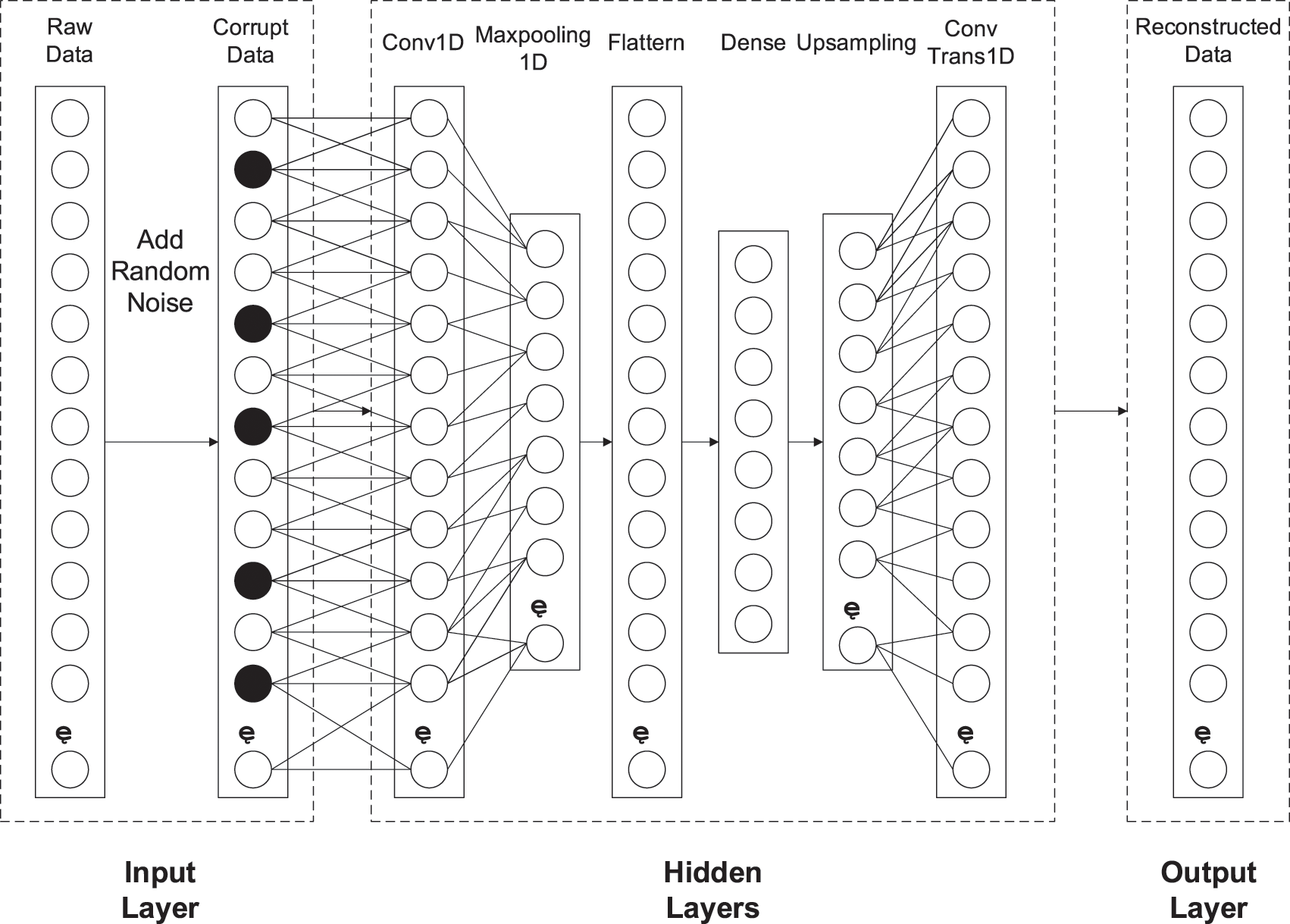
Figure 5: DIFL feature learning model (The name of each layer is displayed at the top). The dense layer is the data after dimensionality reduction

For the input data sample (y=[y1, y2]T) , we randomly insert noise on it to obtain the damaged data (y= [y1′, y2′]T).

The common method of adding noise uses Gaussian noise. In this paper, a certain probability (q) is used to make the value of the input layer node 0:

{P(y~=θy)=1−qP(y~=0)=q (1)

To make corrupted inputs fair, undamaged values are entered with their original values:

θ=1/(1−q) (2)

Next, the damaged data are processed and converted by the activation function to reach the hidden layer. The hidden layer usually has a much smaller data volume than the input data, and this will force the autoencoder to reduce the high-dimensional data to abstract feature data with efficient internal representation.

The input signal is (y∈RD) and the signal after adding noise is y′∈RD) . Inputting the latter signal to the encoder link will get the feature output of the hidden layer:

F=f(ωy′+b) (3)

where (F) is the implicit internal data of the hidden layer, (f) is the encoder transposition function, (ω) is the conversion weight, and (b) is the conversion bias value.

After obtaining the internal data of the hidden layer, the output layer data use the same method to inversely transform the implicit internal data, and the internal data (F) are decoded into output data, (yout∈RD) , which is represented as follows:

yout=g(ω′F+c) (4)

where (yout) is the reconstructed data, (ω′) is the reconstruction weight (c) is the reconstruction offset value, and (g) is the decoder transposition function.

After obtaining the output data, the DIFL will optimize the reconstruction error between the input data and the output data. The parameters (ω) and (ω′) are adjusted to minimize the reconstruction error measured by the loss metric L(y, yout) on the given training set. In our work, we use the mean square error as the loss metric to train the parameters of the DIFL. The loss function is defined as follows:

L(y, y^)=−∑i=1m[yilog⁡y^i+(1−yi)log⁡(1−y^i)] (5)

The equation to minimize the reconstruction error is defined as follows:

minω,ω′LDRL=1P∑P=1P||g(ω′(fω′+b)+c)−Y||L22 (6)

2.3 Classification

This section introduces the classifier used for our deep learning features.

2.3.1 Logistic Regression Classification

Logistic regression classification (LRC) is a linear regression analysis that is currently widely used in medical diagnosis, financial situations, and other fields [18]. The method is simple and intuitive, so it can be easily applied to industrial problems; however, it has poor regression performance for high-dimensional data. Also, there is a problem of underfitting, and accuracy is greatly affected by the quality of the data.

2.3.2 Decision Tree Model

A decision tree model (DT) is a tree structure used in classification and regression. A DT is composed of nodes and directed edges. Generally, a DT contains a root node, several internal nodes, and several leaf nodes. The decision-making process of the DT needs to start from its root node. The data to be tested are compared with the characteristic nodes in the DT, and the next comparison branch is selected according to the comparison result until the leaf node is the final decision result. In this paper, we choose information entropy as our classification criterion because it is the most widely used.

3  Experimental Verification

3.1 Description of the Dataset

A.   SWaT Dataset

The dataset used in the experiment of this paper is the SWaT safety water treatment ICS operating state dataset. The dataset contains the system operating status data contained in the SWaT water treatment process, which includes normal data samples and samples of the system under attack. Data features include the operating status of ICS components such as liquid level indicator transmitter status, flow indicator transmitter status, temperature indicator transmitter status, and solenoid valve status [19]. Since 2015, the dataset has collected a total of more than 50,000 samples, and there is a significant data imbalance problem, which can be a good effect verification of the method proposed in this article.

B.   Bearing dataset

The bearing dataset of Case Western Reserve University is used in this paper. The test stand consists of a 2-hp motor, a torque transducer/encoder, a dynamometer, and control electronics. The test bearings support the motor shaft. Single point faults were introduced to the test bearings using electro-discharge maching with fault diameters of 7, 14, 2, 28, and 40 mils (1 mil = 0.001 inches). SKF bearings were used for the 7, 14, and 21 mils diameter faults, and NTN equivalent bearings were used for the 28 and 40 mil faults [20]. Outer raceway faults are stationary faults; therefore, placement of the fault relative to the load zone of the bearing has a direct impact on the vibration response of the motor/bearing system. In order to quantify this effect, experiments were conducted for both fan and drive bearings with outer raceway faults located at the 3, 6, and 12 o’clock positions [21].

The samples with missing values in the features were removed before data splitting. We tested the model performance in two ways: absolute accuracy and relative accuracy experiments. The case study was carried out on the PYTHON 3.6 platform. We trained our model on a desktop computer with an i7-8700 CPU, 16 GB of RAM, and an Nvidia GTX1080Ti graphics card. Keras was implemented as a deep learning library for the program.

3.2 Comparison Algorithm

3.2.1 Manual Feature Selection

Manual feature selection (MFS) is a method that selects several specific important features from high-dimensional features based on expert experience [22]. Through investigation, we introduced expert experience to extract the 8-dimensional key features: liquid-level indicator transmitter status, flow indicator transmitter status, temperature indicator transmitter status, composition indicator transmitter status, electromagnetic pump status, solenoid valve status, hydraulic valve status, and PLC status. These states cover each key step in the production process. Based on expert experience, these characteristics can effectively assess the security status of the system.

3.2.2 Raw Feature Selection

Raw feature selection (RFS) is a method where we directly use the original high-dimensional feature dataset as the feature set [23]. For industrial control datasets, the original measured values are irregular. We interpolate the measured values to generate a structured original dataset. Therefore, RFS includes 51-dimensional features.

3.2.3 Principal Component Analysis

PCA is one of the commonly used methods to extract low-dimensional features from high-dimensional data. The main idea of the PCA method is to map n-dimensional features to k dimensions to form new orthogonal features [24]. The essence of this method is a k-dimensional feature reconstructed on the basis of the original n-dimensional feature. The goal of PCA is to sequentially find a set of mutually orthogonal coordinate axes from the original space. The choice of new coordinate axes is closely related to the data itself. The number of principal components is usually less than or equal to the number of original variables. In this paper, we apply PCA to the dataset after data processing to generate a feature set based on eight principal component dimensions as a comparison method.

3.2.4 Deep Industrial Feature Learning

DIFL was applied to extract features based on DAE, as introduced in the Methods section. The number of obtained features set was determined by the number of output layers of the encoder network, which could be arbitrary sizes. In this paper, we define a finite unit set U to represent the possible number of hidden layers that can be added. For the industrial control data, we choose U = {2, 3, 4, 5, 6, 7, 8} After some preliminary experiments, we found that using three hidden layers can yield better results by considering the loss error and the classification results. Therefore, we set the number of layers of the encoder network in DIFL to three. Then, we define a finite unit Y = {36, 24, 16, 12, 8, 4, 2} to represent the number of units in the last hidden layer of the encoder network. Finally, we set the number of hidden layer units to be eight. Therefore, for the industrial control dataset, we obtain an encoder network with three hidden layers, and the number of hidden layer units in the last layer of the encoder is eight. After data preprocessing, the original data are input into the DIFL framework, and the generated feature set is eight for each sample.

At the same time, we designed a fully connected DAE, which contains three coding layers and three decoding layers. The activation function of each layer is defined as rectified linear unit (RELU), and the number of overall network layer units is {51, 36, 16, 8, 16, 36, 51}.

3.3 Simulation Experiment Verification

3.3.1 Absolute Accuracy Experiment

The original data were passed through the data preprocessing part, the feature learning part, and the classification part of the framework in succession. To test the absolute accuracy of the feature extraction method in this paper, a convolutional neural network is used as the classification algorithm, and the data after feature extraction are classified after 50 iterations. The results given in this section are average values obtained after multiple experiments with different training and test sets.

Three indicators are used to evaluate the results, namely accuracy and loss. Loss is used to evaluate the degree to which the predicted value of the model is different from the actual value. When training the model with deep learning, it calculates the loss function and updates the model parameters, thereby reducing the optimization error until the loss function value decreases to the target value.

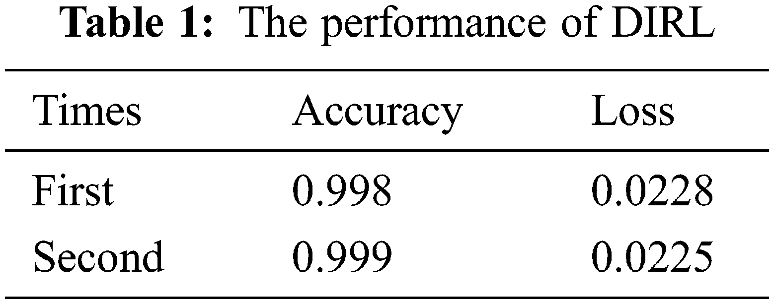
It can be seen in Fig. 6 that the DIFL feature extraction algorithm has good accuracy and fast convergence. The specific values are shown in Table 1. It can be seen that the algorithm provided in this paper guarantees the accuracy, and the degree to which the predicted value of the model is different from the actual value is small.

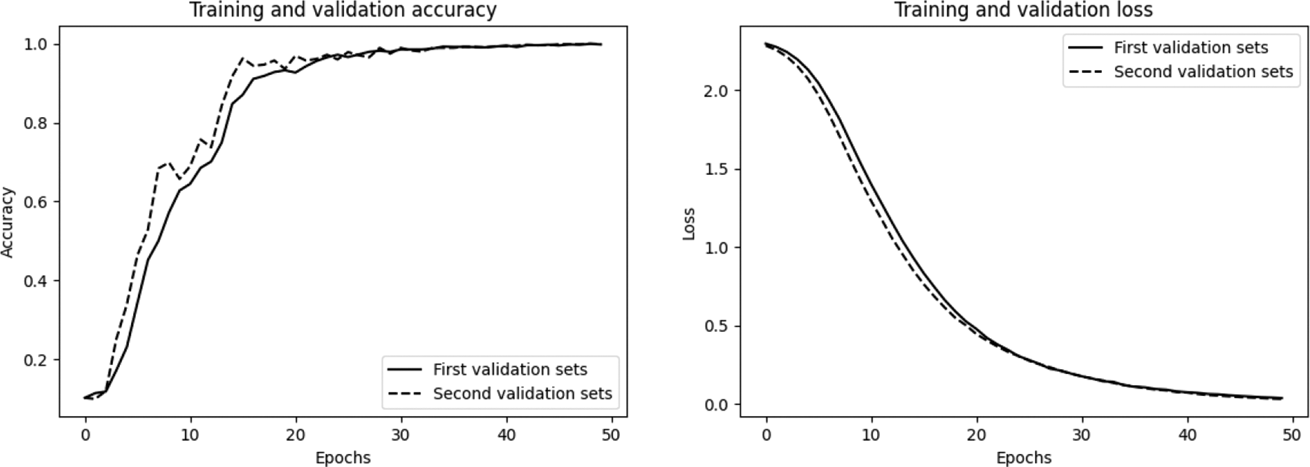
Figure 6: Performance of various feature extraction algorithms (Left: Accuracy, Right: Loss)

3.3.2 Relative Accuracy Experiment

The dataset used in this paper came from the SWaT safe water treatment experimental platform, which has been running since 2015 and is a relatively modern ICS for water treatment.

The staff of the SWaT secure water treatment platform carried out a series of attack behaviors on some transmitters, solenoid valves, and pumps by means of protocol security vulnerabilities; they tampered with their values and realized ICS attack operations. The dataset in this paper was collected under the normal operation of the system and also under data-tampering attack by using the above-mentioned vulnerabilities. The collected data includes the data of the sensors and actuators in the industrial process, as well as the communication network data during the operation of the ICS [25].

In Tables 2 and 3, we compare the performance of classification algorithms using the feature sets determined by the various feature selection methods described in the previous section. Fig. 7 shows the whole workflow of the feature selection experiment.

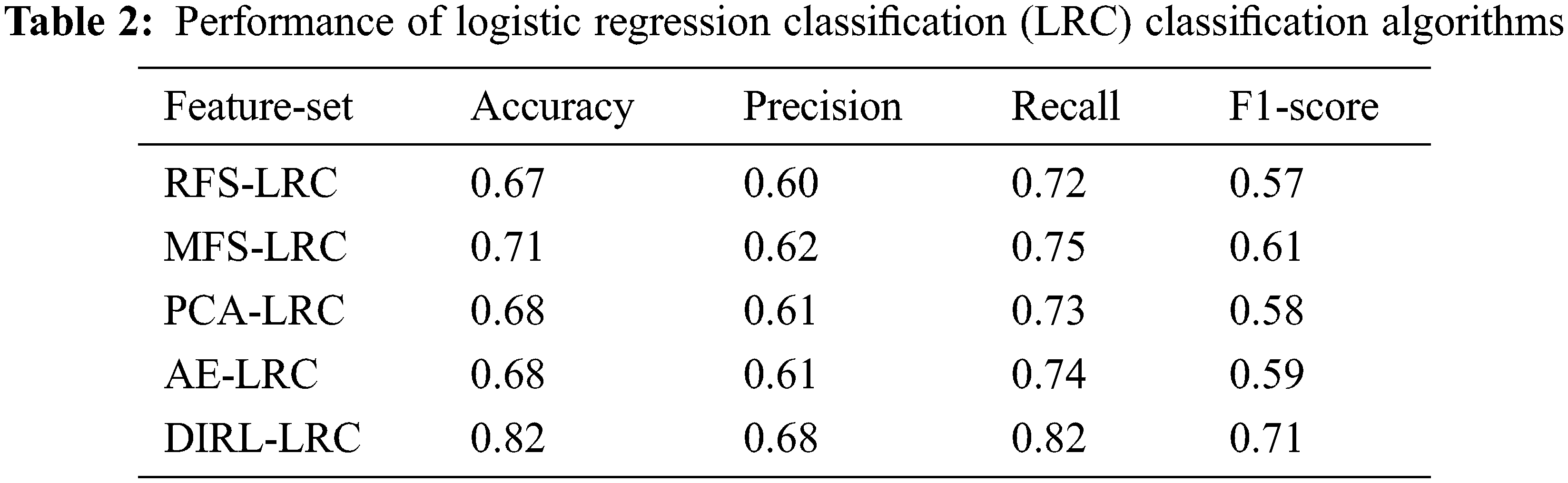
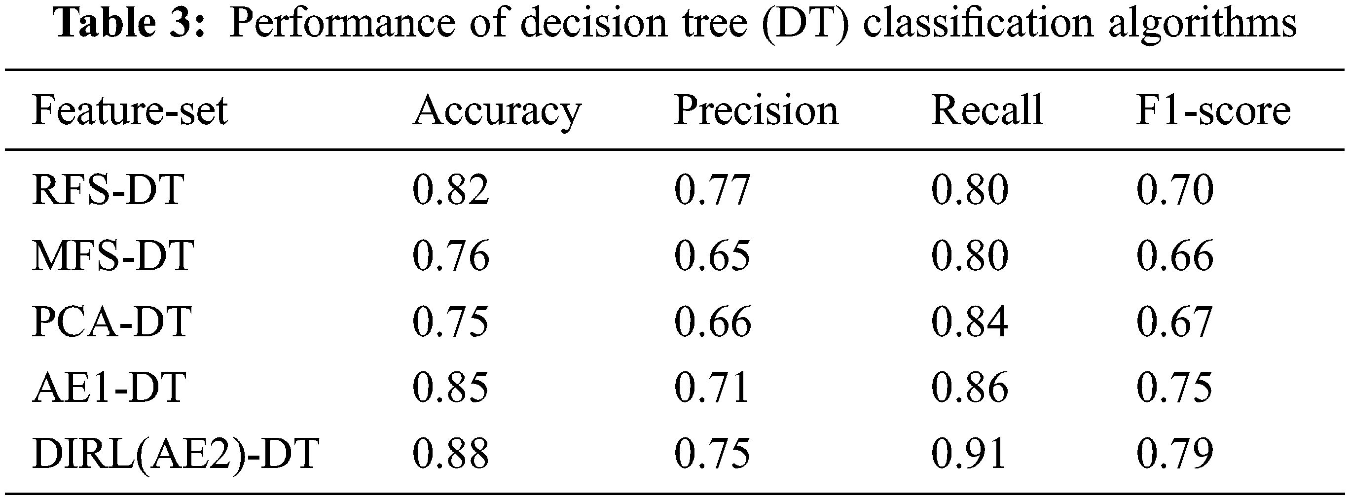
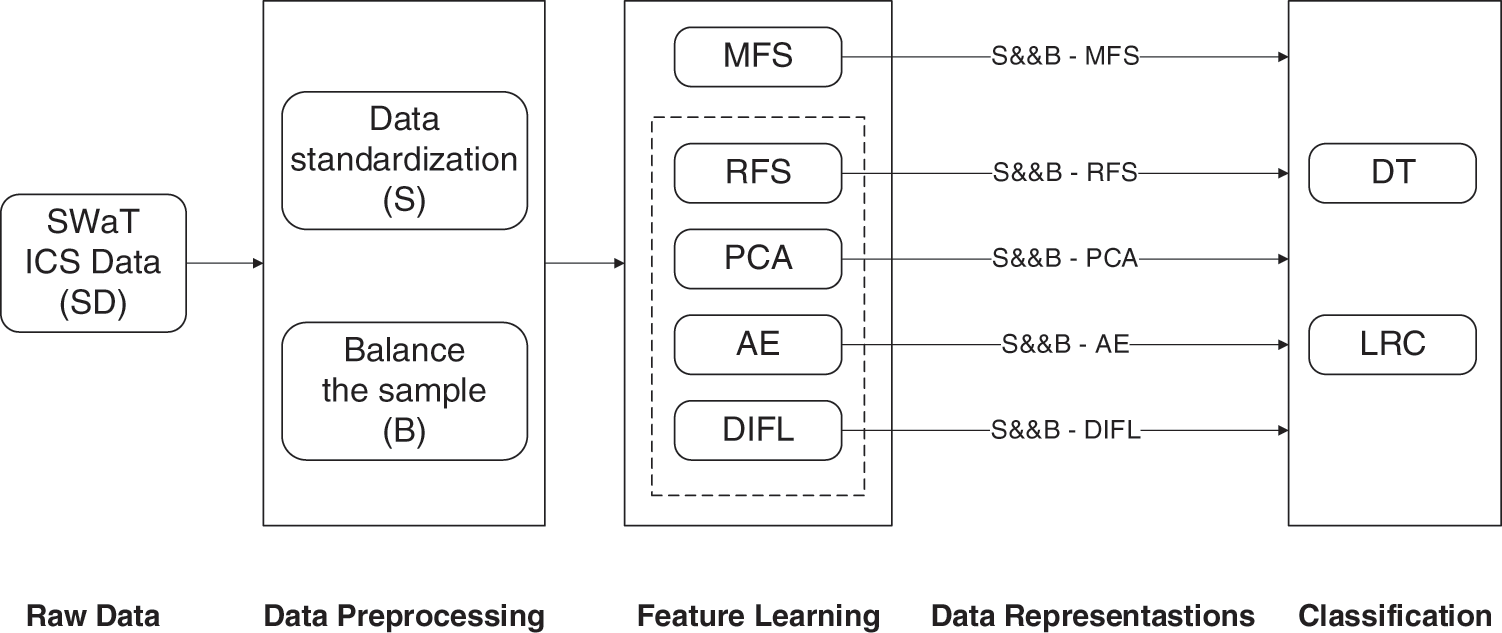
Figure 7: Workflow of the feature selection experiment

The original data were passed through the data preprocessing part, the feature learning part, and the classification part of the framework in succession. There are different sub-blocks in each part, which represent the feature learning and classification methods considered in this paper. Later in the paper, we name the results according to the sub-blocks that each experimental use case passes through. In this paper, to ensure that the test set information is not leaked, the original datasets are divided into 75% go for training and 25% for testing [26], which can make the experimental results more accurate. Only the training set is balanced by data preprocessing. The results given in this section are average values obtained through multiple experiments with different training and test sets.

We mainly use 4 indicators to evaluate the classification results: classification accuracy, precision, recall, and F1-score.

Accuracy, precision, and recall reflect the basic performance of the model, and F1-score is the harmonic mean of precision and recall. The best value of F1-score is 1, and the worst value is 0.

Accuracy=Tp+TNTp+TN+FP+FN,  (7)

precision=TpTP+FP,  (8)

recall=TPTP+FN,  (9)

F1−score=∑i2ωiprecisioni×recalliprecisioni+recalli,  (10)

where ( TP ) is the number of true positives, ( FP ) is the number of false positives, ( TN ) is the number of true negatives, and ( FN ) is the number of false negatives.

Accuracy is the most intuitive indicator to measure the performance of binary classifiers because it represents the probability that the classification result is correct. For an unbalanced dataset, the relationship between the true positive rate and the false positive rate is very important. Therefore, the area under the curve (AUC) of the receiver operating characteristic (ROC) curve should be taken seriously, which is usually used to measure the performance of a classifier constructed from an imbalanced dataset. The higher the AUC of the ROC, the better the classifier performance. The F1 score calculates the average of precision and recall, which is another commonly used indicator to measure the performance of binary classifiers.

Tables 2 and 3 show the classification results using various feature sets and classifiers. Figs. 8 and 9 show the ROC curve and the AUC of each classifier. Table 1 summarizes the results of using logistic regression. We observe that the features extracted by DIRL have the highest classification accuracy. Specifically, the experimental case DIRL-LGC can classify the status of industrial control with 88% accuracy, which is 14% better than that of MFS. The feature learning methods based on deep learning such as AE and DIRL are significantly better than the other feature extraction methods in terms of ROC curve. In addition, it can be seen that the performance of DIRL is generally better than that of AE. This shows that DIRL can better mine the correlation between features for compressed expression by introducing network designs such as a convolutional neural network (CNN) layer and pooling layer. Similar results can be seen from the comparison of AUC-ROC in Fig. 9 and F1 scores in Table 1. The classification results using the DT classifier are shown in Table 2. Similarly, DIRL-DT achieved the best results in all performance indicators. Through the DT classifier, DIRL can achieve the highest classification accuracy—higher than that of all other experimental cases. An interesting observation is that RFS performs better than PCA and AE with DT classifiers. However, its AUC and ROC was not better than the others. This result reflected the unbalanced nature of the datasets. In unbalanced datasets, we should take AUC-ROC as the most important indicator.

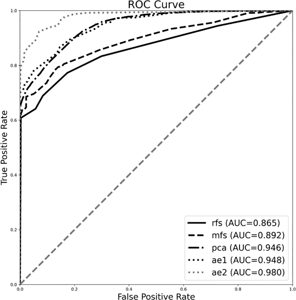
Figure 8: Performance of various feature extraction algorithms classified using the DT method

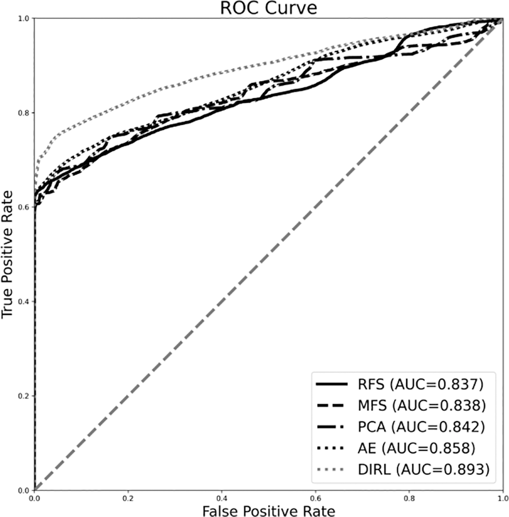
Figure 9: Performance of various feature extraction algorithms classified using the LRC method

4  Conclusion

In this paper, we propose a novel data representation learning model for industrial control systems based on the autoencoder technique. From the experiment results, the DIRL model performed better than other representation learning methods in both absolute accuracy and relative accuracy experiments. The DIRL model can provide a good support for administrators’ decision-making in modern industrial control systems. The advantages of the method proposed in this paper are as follows: (1) the autoencoder network based on CNN can mine the compressed expression of feature samples in the industrial control environment and effectively reduce the dimension of high-dimensional industrial control data; (2) the features obtained from model learning are well suited for state classification of industrial control systems.

This study provides an important contribution to the safety analysis of modern industrial control systems, and the method can be extended to other industrial control data processing tasks. Our future work will focus on providing automatic solutions for ICS management based on our results to maximize information security.

Acknowledgement: Thanks are due to Tao Rui for assistance with the experiments and to Jiang Daqi, Zhang Chunlei for valuable discussion.

Funding Statement: This study is supported by The National Key Research and Development Program of China: “Key measurement and control equipment with built-in information security functions” (Grant No. 2018YFB2004200) and Independent Subject of State Key Laboratory of Robotics “Research on security industry network construction technology for 5G communication” (No. 2022-Z13).

Conflicts of Interest: The authors declare that they have no conflicts of interest to report regarding the present study.

References

1. W. Wang, Z. Wang, Z. Zhou, H. Deng, W. Zhao et al., “Anomaly detection of industrial control systems based on transfer learning,” Tsinghua Science & Technology, vol. 26, no. 6, pp. 821–832, 2021. [Google Scholar]

2. T. T. Huong, T. P. Bac, D. M. Long, T. D. Luong, N. M. Dan et al., “Detecting cyberattacks using anomaly detection in industrial control systems: A federated learning approach,” Computers in Industry, vol. 132, pp. 103509, 2021. [Google Scholar]

3. Y. Lai, J. Zhang and Z. liu, “Industrial anomaly detection and attack classification method based on convolutional neural network,” Security & Communication Networks, vol. 9, pp. 1–11, 2019. [Google Scholar]

4. S. Priyanga, K. Krithivasan, S. Pravinraj and S. V. S. Sriram, “Detection of cyberattacks in industrial control systems using enhanced principal component analysis and hypergraph-based convolution neural network (EPCA-HG-CNN),” IEEE Transactions on Industry Applications, vol. 56, pp. 4394–4404, 2020. [Google Scholar]

5. Y. Bengio, A. Courville and P. Vincent, “Representation learning: A review and new perspectives,” IEEE Transactions on Pattern Analysis & Machine Intelligence, vol. 35, no. 8, pp. 1798–1828, 2013. [Google Scholar]

6. C. Zhou, Y. Jia and M. Motani, “Optimizing autoencoders for learning deep representations from health data,” IEEE Journal of Biomedical and Health Informatics, vol. 23, no. 1, pp. 103–111, 2019. [Google Scholar] [PubMed]

7. P. B. Jensen, L. J. Jensen and S. Brunak, “Mining electronic health records: Towards better research applications and clinical care,” Nature Reviews Genetics, vol. 13, no. 6, pp. 395–405, 2012. [Google Scholar] [PubMed]

8. C. J. Huberty, “Discriminant analysis,” Review of Educational Research, vol. 45, no. 4, pp. 543–598, 1975. [Google Scholar]

9. B. Su and X. Ding, “Linear sequence discriminant analysis: A model-based dimensionality reduction method for vector sequences,” in 2013 IEEE Int. Conf. on Computer Vision, Sydney, NSW, Australia, pp. 889–896, 2013. [Google Scholar]

10. P. Baldi and K. Hornik, “Neural networks and principal component analysis: Learning from examples without local minima,” Neural Networks, vol. 2, no. 1, pp. 53–58, 1989. [Google Scholar]

11. A. S. Tarawneh, C. Celik, A. B. Hassanat and D. Chetverikov, “Detailed investigation of deep features with sparse representation and dimensionality reduction in CBIR: A comparative study,” Intelligent Data Analysis, vol. 24, no. 1, pp. 47–68, 2020. [Google Scholar]

12. M. Alkhayrat, M. Aljnidi and K. Aljoumaa, “A comparative dimensionality reduction study in telecom customer segmentation using deep learning and PCA,” Journal of Big Data, vol. 7, no. 9, pp. 1–23, 2020. [Google Scholar]

13. M. Gnouma, A. Ladjailia, R. Ejbali and M. Zaied, “Stacked sparse autoencoder and history of binary motion image for human activity recognition,” Multimedia Tools and Applications, vol. 78, pp. 2157–2179, 2019. [Google Scholar]

14. W. Jia, K. Muhammad, S. Wang and Y. Zhang, “Five-category classification of pathological brain images based on deep stacked sparse autoencoder,” Multimedia Tools and Applications, vol. 78, no. 4, pp. 4045–4064, 2019. [Google Scholar]

15. A. Tharwat, Y. S. Moemen and A. E. Hassanien, “Classification of toxicity effects of biotransformed hepatic drugs using whale optimized support vector machines,” Journal of Biomedical Informatics, vol. 68, pp. 132–149, 2017. [Google Scholar] [PubMed]

16. K. G. Lore, A. Akintayo and S. Sarkar, “LLNet: A deep autoencoder approach to natural low-light image enhancement,” Pattern Recognition, vol. 61, pp. 650–662, 2017. [Google Scholar]

17. M. Yoshida, T. Shimoda, M. Abe, N. Kakushima, N. Kawata et al., “Clinicopathological characteristics of non-ampullary duodenal tumors and their phenotypic classification,” Pathology International, vol. 69, no. 7, pp. 24–31, 2019. [Google Scholar]

18. K. B. Schebesch and R. Stecking, “Support vector machines for classifying and describing credit applicants: Detecting typical and critical regions,” Journal of the Operational Research Society, vol. 56, no. 9, pp. 1082–1088, 2005. [Google Scholar]

19. N. A. Nguyen, S. Himmelberger, A. Salleo and M. Mackay, “Brush-painted solar cells from pre-crystallized components in a nonhalogenated solvent system prepared by a simple stirring technique,” Macromolecules, vol. 53, no. 19, pp. 8276–8285, 2020. [Google Scholar]

20. S. H. Park, Y. Gao, Y. Shi and D. Sshen, “Interactive prostate segmentation using atlas-guided semi-supervised learning and adaptive feature selection,” Medical Physics, vol. 41, no. 11, pp. 111715, 2014. [Google Scholar] [PubMed]

21. D. Y. Chong, H. J. Kim, P. Lo, S. Young, M. Gray et al., “Robustness-driven feature selection in classification of fibrotic interstitial lung disease patterns in computed tomography using 3D texture features,” IEEE Transactions on Medical Imaging, vol. 35, no. 1, pp. 144–157, 2015. [Google Scholar] [PubMed]

22. W. B. Wang, Z. Y. Tian and S. Y. Wang, “Application of cross sectional PCA in boiler fault diagnosis,” Information and Control, vol. 49, no. 4, pp. 6, 2020. [Google Scholar]

23. W. Mao, Y. Chiu, C. Chu, B. Lin and J. Hung, “Dynamic sliding mode backstepping control for vertical magnetic bearing system,” Intelligent Automation & Soft Computing, vol. 32, no. 2, pp. 923–936, 2022. [Google Scholar]

24. Y. M. Zhai, A. D. Deng, J. Li, Q. Cheng and W. Ren, “Remaining useful life prediction of rolling bearings based on recurrent neural network,” Journal on Artificial Intelligence, vol. 1, no. 1, pp. 19–27, 2019. [Google Scholar]

25. X. Pan, Z. Wang and Y. Sun, “Review of PLC security issues in industrial control system,” Journal of Cyber Security, vol. 2, no. 2, pp. 69–83, 2020. [Google Scholar]

26. J. L. Medina-Franco, A. Golbraikh, S. Oloff, R. Castillo and A. Tropsha, “Quantitative structure-activity relationship analysis of pyridinone HIV-1 reverse transcriptase inhibitors using the k nearest neighbor method and QSAR-based database mining,” Journal of Computer-Aided Molecular Design, vol. 19, no. 4, pp. 229, 2005. [Google Scholar] [PubMed]