Framework for a Computer-Aided Treatment Prediction (CATP) System for Breast Cancer

1  Introduction

In 2020, 2.3 million women were diagnosed with breast cancer, with 68,500 worldwide fatalities. As of 2020, 7.8 million women have been diagnosed with breast cancer in the past five years, making it the world’s most prevalent cancer [1]. In clinical terms, malignant tumours are typically classified as positive, whereas benign tumours are classified as negative. Both cancers have subgroups that must be identified separately since each might have a different prognosis and treatment plan. Accurate identification of each subcategory is required for proper diagnosis. Mammography, ultrasound, magnetic resonance imaging (MRI), computed tomography (CT), positron-emission tomography (PET), and microwave imaging are now used in the diagnosis of breast cancer [2–7]. There are two types of breast cancer manifestations in medical images: masses and calcifications. On appearance, benign tumours are often spherical, smooth, and transparent. Calcification has a coarser form, a granular shape, a popcorn shape, or a ring shape, and it has a greater density and a more scattered dispersion. The margins of typical malignant tumours are uneven and typically fuzzy, and the mass has a needle-like appearance. Calcification has a morphology that is generally sand-like, linear, or branching, with various forms and sizes. The distribution is usually dense or clustered in a linear pattern [8–10]. Fig. 1 shows a picture of malignant and benign breast cancer.

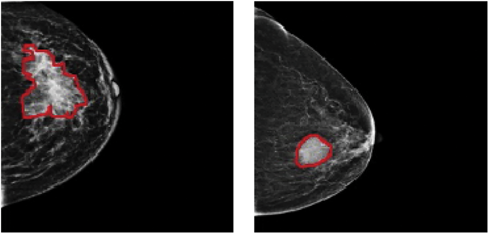
Figure 1: (Left) Malignant and (Right) benign breast cancer images

Since the late 1960s, computer-aided diagnosis (CAD) for mammography has progressed. Its primary goal is to aid radiologists in detecting malignancies that might otherwise go undetected [2]. CAD programs identify high-density regions and microcalcifications. Computer-aided detection systems (CADe) and computer-aided diagnostic systems (CADx) are the two types of CAD systems. The localization job (identification of a suspicious abnormality) is the focus of CADe, which acts as a second reader for radiologists and leaves patient care decisions to the radiologist. However, CADx classifies an abnormality detected by a radiologist or a computer, estimating the likelihood of an abnormality and classifying it as benign or malignant. The radiologist next evaluates if the anomaly deserves additional investigation and the clinical relevance of the finding [6]. In 1998, the US Food and Drug Administration (FDA) approved the first CAD software for screening mammography, R2 Image Checker, made by R2 Technologies (now known as Hologic) [11]. Early findings were encouraging [12,13] and by 2016 CAD has become extensively used in clinical practice, with roughly 92% of all mammography facilities in the United States adopting it [14]. However, its clinical use is debatable, owing to the high percentage of false-positive results [15].

Image identification, clinical translation of tumour phenotype to genotype, and outcome prediction in connection to treatment and prognosis strategies are areas where artificial intelligence (AI) can streamline and integrate radiologist diagnostic skills. For decades, radiologists have relied on AI-assisted CAD systems to translate visual data to quantitative data [16–18]. Such technologies have the potential to significantly reduce the amount of time and effort necessary to analyse a lesion in clinical practice, as well as the number of false positives that result in painful biopsies without compromising BC detection sensitivity [7,19,20]. Predicting the proper treatment plan is an area that needs improvement in terms of CATP that can be used as a decision support system in clinical practice. In recent years, the clinical community's increased adoption of health information technology has opened new opportunities and possibilities for employing sophisticated Clinical Decision Support (CDS) systems. CDS systems can be defined as ‘‘systems that are designed to be a direct aid to clinical decision-making in which the characteristics of an individual patient are matched to a computerized clinical knowledge base, and patient-specific assessments or recommendations are then presented to the clinician(s) and/or the patient for a decision’’ [21]. Memorial Sloan Kettering (MSK) trained IBM Watson for Oncology (WFO) is a CDS system that is meant to aid medical oncologists in making expert treatment recommendations based on crucial disease and patient-specific characteristics. WFO can include complexities not addressed by existing recommendations, thanks to medical logic taught by MSK and IBM Watson’s machine learning on genuine and synthetic MSK cases. Breast surgery, radiotherapy, clinical genetics, and fertility preservation are all factors to consider while deciding on adjuvant systemic therapy for early-stage breast cancer. [22] Studies, however, have shown a low level of concordance between WFO and the recommendations done by the Multidisciplinary Team (MDT) for advanced breast cancer stages [23]. MATE, or Multidisciplinary Team Assistant and Treatments Elector, is an another CDS system that was created for breast multidisciplinary team meetings and tested in the London Royal Free Hospital to aid patient-centered, evidence-based decision-making [24]. Even though CDS systems are becoming increasingly important in improving treatment and cutting costs, there is little evidence to support their widespread use and effectiveness. Many studies were carried out in academic settings, on a small number of patients, or specific stages of cancer, with most of them being examined in ambulatory settings. In a variety of situations and systems, clinical decision support enhanced medication prescribing, the facilitation of preventative care services, and the ordering of clinical research. Among these studies, very few are related to breast cancer CDS and thus to stimulate wider use of such systems and increase their therapeutic effectiveness, more research is needed [23,25].

This paper proposes an opensource framework for a CATP system for breast cancer. Fig. 2 depicts a diagram of the proposed framework that is composed of two phases: Classification Phase and Prediction Phase. Classification phase starts with selecting the dataset, cleaning the data, feature engineering and preparing the training and testing data. After that, four classification models are tested on the training data and their performance is evaluated, the best performing model will be selected to be used in phase two. The prediction phase will use the best selected model from phase one to predict the treatment plan using the test data and new data.

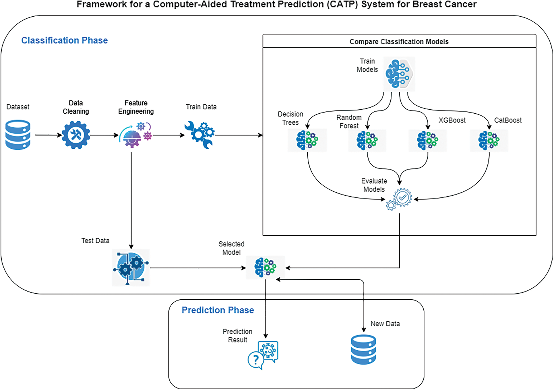
Figure 2: Framework for a computer-aided treatment prediction system (CATP) for breast cancer

The contents of this paper are organized as follows: Section 2 reviews previous work on breast cancer, its diagnosis, and treatment. Section 3 contains the experimental setup details, dataset used, classification models, and the evaluation metrics. In Section 4, we present a series of experimental results to demonstrate the effectiveness of the proposed framework. Finally, concluding remarks are provided in Section 5.

2  Breast Cancer: Diagnosis and Treatment

2.1 Breast Cancer

Breast cancer is a condition in which the cells of the breast begin to grow out of control. There are several types of breast cancer. The kind of breast cancer is determined by which cells in the breast become cancerous. Breast cancer can start in a variety of places in the breast. Lobules (glands that make milk), ducts (tubes that transport milk from the breast to the nipple), and connective tissue (fibrous and fatty tissue) are the three major components of a breast. Breast cancer usually starts in the ducts or lobules, it can also spread to other parts of the body via blood and lymph arteries. In situ or non-invasive cancer cells remain inside the basement membrane of the components of the terminal duct lobular unit and the draining duct. Breast cancer that has spread outside the basement membrane of the ducts and lobules into the surrounding normal tissue is known as invasive breast cancer and is considered to have metastasized [26–28].

2.2 Breast Cancer Diagnosis

Breast cancer is divided into three categories based on Estrogen receptor (ER), Progesterone receptor (PR), and human epidermal growth factor 2 (ERBB2) gene amplification, previously known as human epidermal growth factor receptor 2 (HER2) gene amplification: ER or PR positive (also known as HR+), ERBB2 positive, or triple negative. HR+ or ERBB2+ subtypes have a five-year average overall survival, while triple-negative subtypes have a one-year average overall survival [29]. Each of the three subtypes has its own set of risks and treatment options. The best treatment for each patient is determined by their tumour subtype, anatomic cancer stage, and personal preferences [30].

There are several cancer staging methods in use right now. One method divides tumours into four stages: Stage 0, Stage I, Stage II, Stage III, and Stage IV, with further subcategories, where Stage IV denotes a metastatic distant cancer. TNM (tumour, node, metastasis) is another cancer staging method that assigns stages based on the tumour, node and metastases status [31]. Stage I breast cancer, defined anatomically as a breast tumour smaller than 2 cm and no lymph node involvement, have five years survival rate of at least 99% for HR+, at least 94% for ERBB2+, and at least 85% for triple-negative subtypes [32].

2.3 Breast Cancer Treatment

There are two types of treatment for cancer, depending on the kind and stage of the disease: local and systemic. Surgery and radiation are considered local treatments as they treat the tumour without harming the rest of the body. Systemic therapy, on the other hand, employs the use of medicines to combat the disease. Drugs can reach cancer cells anywhere in the body and be administered directly into the bloodstream or orally. Systemic treatments include chemotherapy, hormone therapy, targeted medication therapy, and immunotherapy. Systemic treatment maybe preoperative (neoadjuvant), postoperative (adjuvant), or both [30,33,34]. Most patients will have a combination of local treatments to control local disease and systemic treatment for any metastatic disease.

2.3.1 Surgery

Breast conservation surgery (excision of the tumour with surrounding normal breast tissue) or mastectomy (removal of the entire breast) are two options for surgery (total removal of breast tissue). Because of their impact on local recurrence following breast-conserving surgery, some clinical and pathological variables may affect breast conservation or mastectomy choices. An inadequate initial excision, young age, the existence of a significant in situ component, lymphatic or vascular invasion, and histological grade are all factors to consider. Local recurrence is two to three times more probable in young individuals (under 35) than in older patients. While other risk factors for local recurrence are more common in young individuals, young age appears to be an independent risk factor [35].

Mastectomy

Mastectomy is a surgical procedure that removes the breast tissue and a portion of the underlying skin, which generally includes the nipple. A mastectomy should be paired with axillary lymph nodes surgery in some way. Lymph node ectomy is used for both diagnostic (determining the anatomic extent of breast cancer) and therapeutic purposes (removal of cancerous cells) [30]. About a third of locally advanced breast cancers are unsuitable for breast conservation surgery but may be treated with mastectomy. Some patients who are candidates for breast conservation surgery choose mastectomy instead. Until the demonstration of equivalent outcomes with mastectomy and breast-conserving surgery plus irradiation against the remaining breast in patients, mastectomy was the primary surgical treatment employed in the vast majority of patients [26,35].

Breast Conservation Surgery

Breast conservation surgery may consist of excision of the tumour with a 1 cm margin of normal tissue (broad local excision) or a more extensive excision of a complete quadrant of the breast (breast conservation surgery) (quadrantectomy). The extent of excision is the most critical factor that determines local recurrence following breast-conserving. Compared to grade II or III tumours, grade I tumours have a 1.5-fold reduced recurrence rate. The lower the recurrence rate, but the poorer the aesthetic effect, the larger the excision. Although there is no size restriction for breast conservation surgery, adequate excision of lesions larger than 4 cm yields a poor aesthetic outcome. Hence most breast units limit breast-conserving surgery to lesions less than 4 cm. Breast conservation surgery may be done at any age [26,36,37].

2.3.2 Radiotherapy

Breast cancer patients may get radiation treatment to the entire breast or a breast section (after lumpectomy), the chest wall (after mastectomy), and the regional lymph nodes. Whole-breast radiation after a lumpectomy is a standard part of breast-conserving treatment [38]. After breast conservation surgery, postoperative radiotherapy is strongly advised. Whole breast radiation therapy alone lowers the 10-year risk of any first recurrence (both local and distant) by 15% and the 15-year risk of breast cancer-related death by 4% [37]. Radiation to the chest wall, occasionally with a boost to the mastectomy scar and regional nodal radiation, is known as postmastectomy radiation (PMRT). PMRT lowers the 10-year risk of recurrence (including locoregional and distant) by 10% and the 20-year risk of breast cancer-related death by 8% in node-positive patients. The advantages of PMRT are unaffected by the number of implicated axillary lymph nodes or the use of adjuvant systemic therapy [39].

2.3.3 Systemic Treatment

In the United States, 5.8% of breast cancer patients are metastatic, with a 5-year survival rate of 29% [40]. The best treatment for metastatic breast cancer (MBC) remains a substantial therapeutic problem; the best medical therapy for each patient must be chosen based on breast cancer risk assessment, predictive indicators, toxicity risk, and patient preferences [41]. Adjuvant systemic treatment should begin as soon as possible following surgery, preferably within 2–6 weeks [37]. There are a few broad guidelines to follow: in metastatic HR+/HER2 breast cancer, early treatment should be centred on endocrine therapy (ET). Patients are transitioned to chemotherapy (CT) after developing resistance to the available hormonal therapies [42]. ET is still the most effective treatment for hormone-sensitive, non-life-threatening MBC. This systemic medication offers the benefits of effectiveness, low toxicity, and high quality of life [41]. ET is used in clinical practice when the primary tumour or, if possible, a readily accessible metastasis ER+, PR+, or HR+. When the danger of rapid disease development is modest, i.e., there is no life-threatening sickness, this sort of therapy is typically the first choice [30]. CT is presently the sole treatment option for women with endocrine resistant illnesses who are ER- and HER2- [43].

Neoadjuvant chemotherapy is used to treat localized early-stage triple-negative breast cancer (TNBC) to preserve the breast or for patients who are temporarily unable to undergo surgery. Chemotherapy in the neoadjuvant situation allows for a direct clinical examination or imaging evaluation of the response [44]. TNBC has a more significant percentage of pathologic complete response (PCR) after neoadjuvant chemotherapy than HER2- illness (28%–30% vs. 6.7%) [42].

3  Materials and Methods

3.1 Dataset

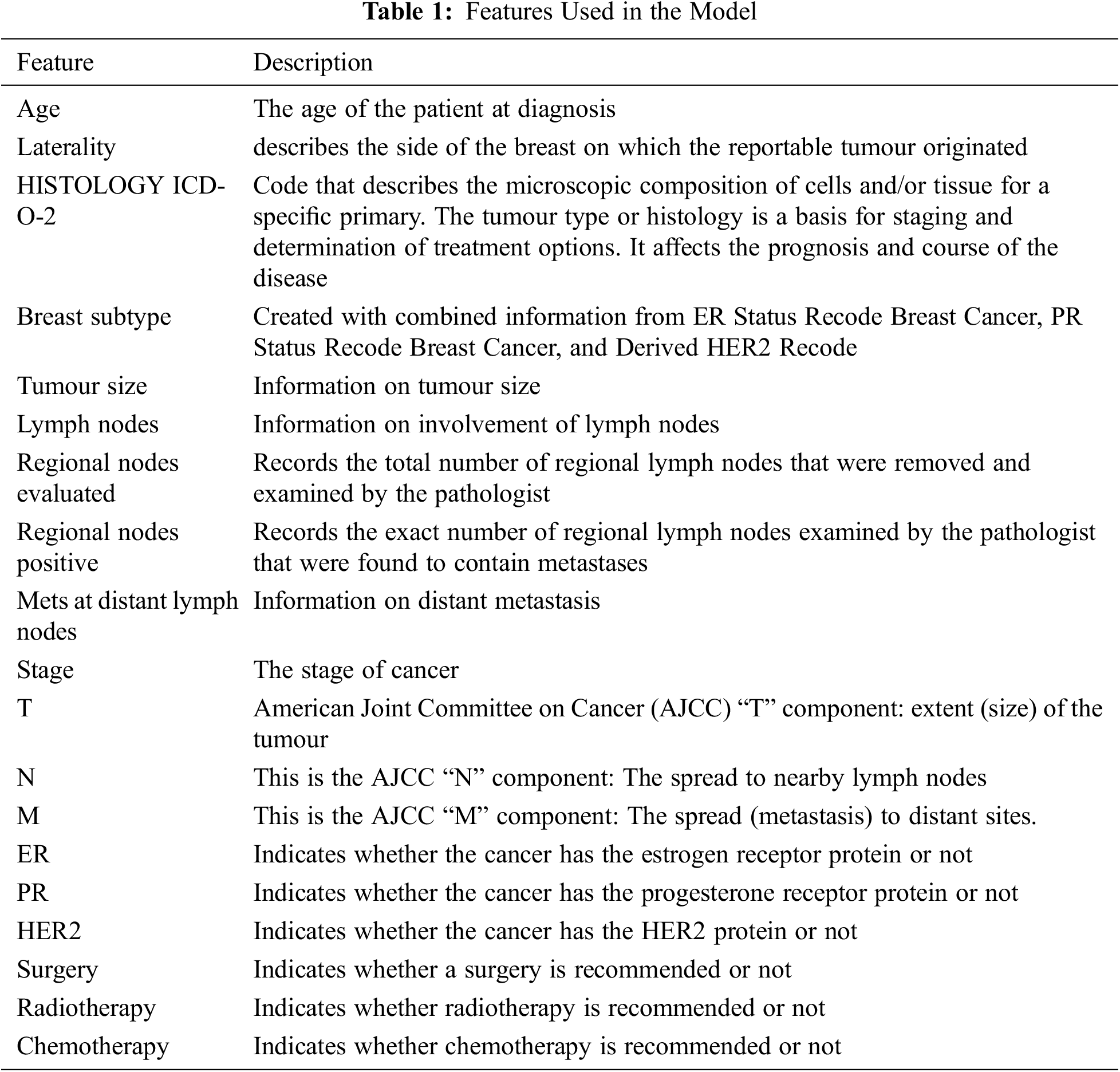
The Surveillance, Epidemiology and End Results (SEER) Program of the National Cancer Institute (NCI) is a trustworthy source of information on cancer incidence and survival in the United States. SEER now collects and publishes cancer incidence and survival data from community-based cancer registries covering about 47.9% of the US population. The SEER Program registries routinely gather data on patient demographics, initial tumour site, tumour shape and stage at diagnosis, the first course of therapy, and vital status follow-up [45]. The data is publicly available and can be obtained after signing a data use agreement. Its latest version covers identified cancer incidences from years 1973 through 2018. In 2018 there were an estimated 3,676,262 women living with female breast cancer in the United States, the rate of new cases of female breast cancer was 129.1 per 100,000 women per year. The death rate was 19.9 per 100,000 women per year [46]. This work utilized the SEER research plus data released in November 2020, which contains records between 1992 and 2018. The extracted data set, after feature engineering and data cleaning, includes 336,525 records, with each record having 19 features, see Table 1, including the patient age category, features related to the tumour and extent of disease, in addition to 3 features representing the three treatment modalities (Surgery, Radiotherapy, and Chemotherapy).

3.2 Treatment Classes Extraction

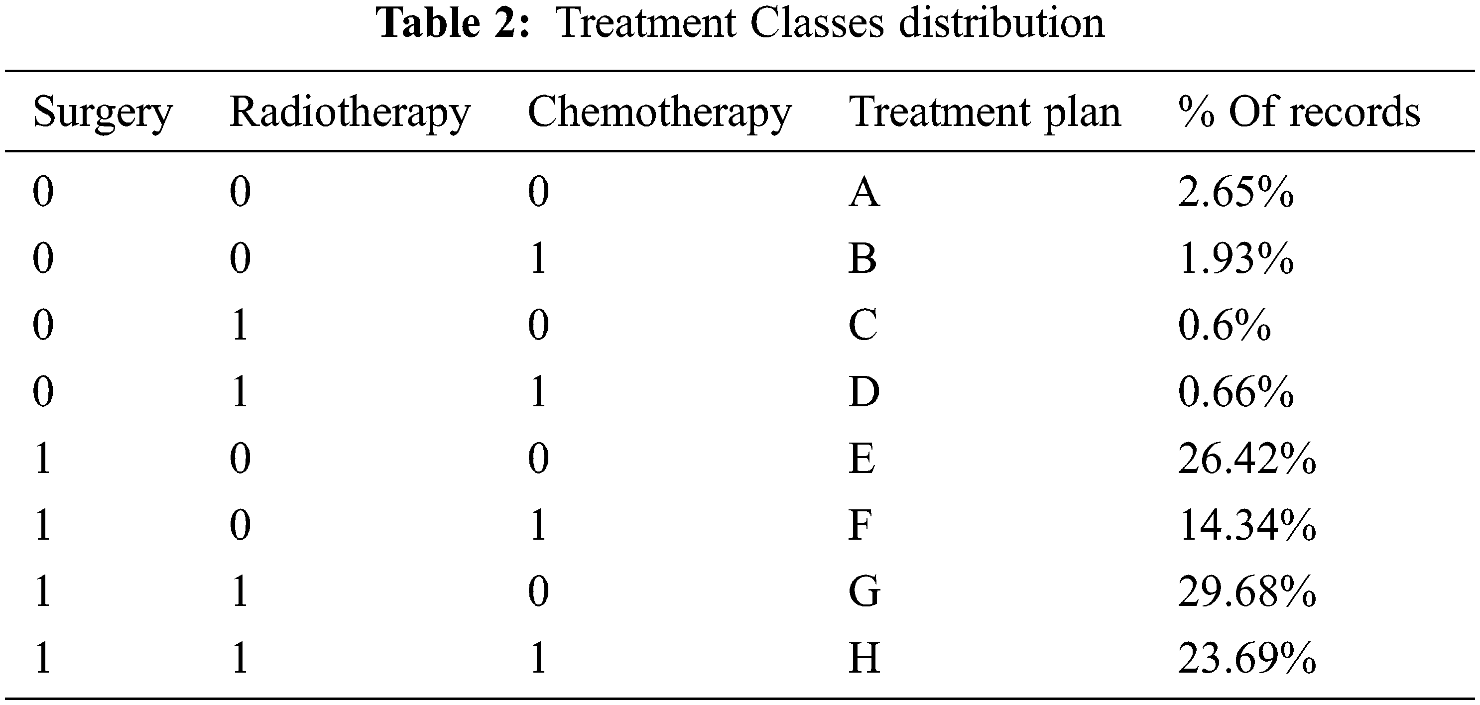
To prepare the data for the model, and since we are only interested in whether a specific treatment is recommended or not, the information in the three treatment features (Surgery, Radiotherapy, and Chemotherapy) was converted into binary (yes/no). After considering the different treatment combinations, we ended up with eight classes representing the various treatment plans. Table 2 summarizes the plans and their distribution in the dataset, which shows that the result dataset is imbalanced.

After generating the plans, the three treatment features will be removed from the dataset and thus ending up with sixteen features that will be used in the proposed models. The newly extracted feature will be used as the label for our model.

3.3 Feature selection

The goal of feature selection is to pick a subset of features from the input that can accurately characterize the data while limiting the influence of noise and irrelevant variables and still delivering high prediction results. Feature selection has been shown to be an effective and efficient data preparation approach for preparing data (particularly high-dimensional data) for machine-learning problems [47–49]. Feature selection have been used in cancer detection models [50,51] as well as for breast cancer detection models [52]. In this work, we will be testing different feature selections algorithms. Feature importance is calculated as the decrease in node impurity weighted by the probability of reaching that node.

Recursive Feature Elimination (RFE): is a recursive process that ranks features according to some measure of their importance. At each iteration, the importance of each feature is measured, and the least relevant one is removed [53,54].

Shapley Additive exPlanations (SHAP) method: based upon the Shapley value concept from game theory [55]. Several approaches to applying the Shapley value to the problem of feature importance have been presented. Given a model f(x1,x2,…,xd ), the features from 1 to d might be regarded participants in a game where the payoff v is some measure of the relevance or impact of that subset. The Shapley value ∅v(i) can thus be thought of as impact of i on the result [56].

Shap-hypetune: is a library that integrates hyperparameter tuning with feature selection in a single pipeline to optimize the optimal number of features while looking for the best parameter configuration. Hyperparameter tuning and feature selection may also be performed independently [57].

A feature selection criterion that can measure the relevance of each feature with the output class/labels is necessary to eliminate an irrelevant feature. If a system employs irrelevant variables in machine learning, it will apply this knowledge for new data, resulting in poor generalization. Other dimension reduction approaches, such as Principal Component Analysis (PCA), should not be compared to removing irrelevant variables because good features might be independent of the rest of the data [49].

3.4 Classification Models

After selecting the features, the input samples are classified into one of the treatment classes using a classifier. In this study we will utilize Decision Trees (DT), Random Forest (RF), XGBoost, and CatBoost (gradient boosting on decision trees) to predict the treatment plan.

Decision Trees: Decision trees are logically combined sequences of basic tests in which each test compares a numeric attribute to a threshold value or a nominal attribute to a range of alternative values. A decision tree identifies a data item as belonging to the most frequent class in a partitioned region when it falls inside that region [58–60]. Several methods have been developed to assess the degree of inhomogeneity, or impurity, entropy and the Gini index are the two most frequent measurements for decision trees. Assume we’re attempting to categorize things into m classes using a set of training items E. Let pi (i = 1,…,m) be the fraction of the items of E that belong to class i. The entropy of the probability distribution (Pi)i=1m gives a reasonable measure of the impurity of the set E. The entropy, −∑i=1m⁡pilog⁡pi , is lowest when a single pi equals 1 and all others are 0, whereas it is maximized when all the pi are equal. The Gini index [60], another common measure of impurity, is computed by 1−∑i=1m⁡pi2 . This is again zero when the set E contains items from only one class. Given a measure of impurity I, we choose a test that minimizes the weighted average of the impurity of the resulting children nodes. That is, if a test with k possible answers divides E into subsets E1…, Ek, we choose a test to minimize ∑j=1k⁡(|Ej|/|E|)I(Ej) . In many cases, we can choose the best test by enumerating all possibilities. If I is the entropy function, then the difference between the entropy of the distribution of the classes in the parent node and this weighted average of the children’s entropy is called the information gain. The information gain, which is expressible via the Kullback-Leibler divergence [59], always has a nonnegative value. Limiting the complexity of the trained trees so that they do not overfit the training instances is an essential part of using decision trees. Stopping splitting when no test enhances the purity of the subgroups by more than a bit of amount is one strategy. Alternatively, we can opt to build out the tree until no more leaves can be subdivided. In this instance, we must prune the tree by eliminating nodes to avoid overfitting the training data. Other approaches, which rely on concepts like minimal description length [59,60], remove nodes in an attempt to explicitly balance the complexity of the tree with its fit to the training data, can also be considered. Cross-validation on left-out training examples should be used to ensure that the trees generalize beyond the examples used to construct them.

Random Forest: is a classification approach that uses an ensemble of data. It develops hundreds of different classification trees and combines them into a composite classifier. The majority rule is used to the votes of the individual classifiers to determine the final classification of a given sample. Each tree is constructed using only a smaller sample (a bootstrap) of the training data to create uncorrelated and dissimilar predictions. Furthermore, the method includes randomization in searching for the optimal splits to boost the variety between them [52,61]. The base learner of RF is a binary tree constructed using recursive partitioning (RPART) in which binary splits recursively partition the tree into homogeneous or near homogeneous terminal nodes. A successful binary split sends data from a parent tree-node to its two daughter nodes, improving the homogeneity of the daughter nodes resulting from the parent node [54]. Given an ensemble of classifiers h1(x), h2(x), …,hk(x) , and with the training set drawn at random from the distribution of the random vector X, Y, define the margin function as:

mg(X, Y)= avkI(hk(X)=Y)−maxj≠Y⁡avkI(hk(X)=j) (1)

where I(.) is the indicator function. The margin indicates the average number of votes for the correct class at X, Y outnumbers the average vote for any other class. The greater the margin of error, the more confident the categorization is. The generalization error is calculated as follows:

PE∗=PX,Y(mg(X,Y)<0) (2)

where the subscripts X, Y indicate that the probability is over the X, Y space. The more trees are added, RF produces a limiting value of the generalization error, and thus, no overfitting occurs [54,61].

eXtreme Gradient Boosting (XGBoost): is an implementation of gradient boosting algorithm [62]. This algorithm works on an intriguing approach known as “boosting”, which combines the performance of numerous “weak” classifiers to build a powerful “committee”. XGBoost is available as an open-source package [63] and have been used widely in research [62,64,65]. The tree ensemble model includes functions as parameters and cannot be optimized using traditional optimization methods in Euclidean space. Instead, the model is trained in an additive manner. Formally, let y^i(t) be the prediction of the ith instance at the tth iteration, we will need to add ft to minimize the following objective:

ℒ(t)= ∑i=1n⁡l(yi,y^i(t−1)+ft(xi))+Ω(ft) (3)

This means we greedily add the ft that most improves our model. Second-order approximation can be used to quickly optimize the objective in the general setting:

ℒ~t=∑i=1n⁡[gift(xi)+12hift2(xi)]+Ω(ft) (4)

where gi=∂y^(t−1)l(yi,y^i(t−1)) and hi=∂2y^(t−1)l(yi,y^i(t−1)) are first and second order gradient statistics on the loss function.

Define Ij={i|q(xi)=j} as the instance set of leaf j . We can rewrite the previous equation by expanding Ω as follows:

ℒ~t=∑j=1T⁡[(∑i∈Ij⁡gi)ωj+12(∑i∈Ij⁡hi+λ)ωj2]+γT (6)

For a fixed structure q(x) , we can compute the optimal weight ωj∗ of leaf j by:

ωj∗=−∑i∈Ij⁡gi∑i∈Ij⁡hi+λ (7)

And calculate the corresponding optimal value:

ℒ~t(q)=−12∑j=1T(∑i∈Ij⁡gi)2∑i∈Ij⁡hi+λ+γT (8)

This equation can be used as a scoring function to measure the quality of a tree structure q. This score is like the impurity score for evaluation decision trees, except that it is derived for a wider range of objective functions.

CatBoost: is an open-source decision tree gradient boosting technique. It was created by Yandex researchers and engineers and used by Yandex and other organizations such as CERN, Cloudflare, and Careem taxi for search, recommendation systems, personal assistant, self-driving vehicles, weather prediction, and many more other activities [66]. This library successfully handles categorical features and surpasses current publicly available gradient boosting algorithms in terms of quality. CatBoost employs a more efficient technique that minimizes overfitting and allows the entire dataset to be used for training [67,68]. Assume you are given a dataset of observations 𝒟={(Xi,Yi)}i=1..n where Xi=(xi,1,…,xi,m) is a vector of m features, some numerical, some categorical, and Yi∈R is a label value. Let σ=(σ1, …, σn) be the permutation, then xσp,k is substituted with:

∑j=1p−1⁡[xσj,k=xσp,k]Yσj+a.P∑j=1p−1⁡[xσj,k=xσp,k]+a (10)

where P is a prior value and a > 0 is a weight of the prior. Each new tree in CatBoost, like all other gradient boosting implementations, is built to approximate the gradients of the existing model. However, due to the problem of biased pointwise gradient estimations, all classical boosting methods suffer from overfitting. To solve this issue, CatBoost uses unbiased estimate of the gradient step. Let Fi be the model constructed after building first i trees, gi(Xk,Yk) be the gradient value on the kth training sample after building i trees. To make the gradient gi(Xk,Yk) unbiased with respect to the model Fi , then the model Fi should be trained without the observation Xk .

3.5 Model Evaluation

Learning algorithm evaluation is not a simple task, as it needs a careful selection of assessment metrics, error-estimation methodologies, statistical tests, and a realization that the results will never be entirely conclusive. This is due, in part, to any evaluation tool's inherent bias and the frequent violation of the assumptions on which it is based. When there are class disparities, as there are in the dataset utilized in this study, the problem becomes considerably more complex. When data is skewed, the default, relatively robust techniques employed for un-skewed data may fail catastrophically [69]. Because standard metrics are intolerant to skewed domains, using them in imbalanced domains might result in sub-optimal classification models and sometimes misleading findings [70]. Three families of assessment metrics used in the context of classification have been identified by several machine learning researchers. The threshold metrics (e.g., accuracy, sensitivity-specificity metrics, and precision-recall metrics (F-measure)), ranking techniques and metrics (e.g., Receiver Operating Characteristic (ROC) analysis and AUC), and probabilistic metrics (e.g., log loss (cross entropy), root-mean-squared error) are all examples of these. The most commonly used metric in imbalanced learning is the AUC-ROC curve [69–72]. The notion of ROC analysis might be construed as follows in the context of the problem of class imbalance. Imagine that instead of training a classifier at a single degree of class imbalance, it is trained at all potential levels of imbalance. The true positive rate (or sensitivity) and the false positive rate are taken as a pair for each of these levels (FPR), where:

True Positive Rate (TPR)= True Positive(True Positive+False Negative) (11)

False Positive Rate (FPR)= False Positive(False Positive+True Negative) (12)

where True Positive and True Negative is the number of samples which are correctly identified as positives or negatives by the classifier in the test set, respectively, and False Negative and False Positive represent the numbers of samples corresponding to those cases as they are mistakenly classified as benign or malignant, respectively. The points represented by all the acquired pairings are shown in what is known as the ROC space, a graph that depicts the true positive rate as a function of the false positive rate. The dots are then connected to form a smooth curve that reflects the classifier’s ROC curve. The closer a curve representing a classifier is from the top left corner of the ROC space (small FPR, large TPR) the better the performance of that classifier. For example, f1 performs better than f2 in Fig. 3.

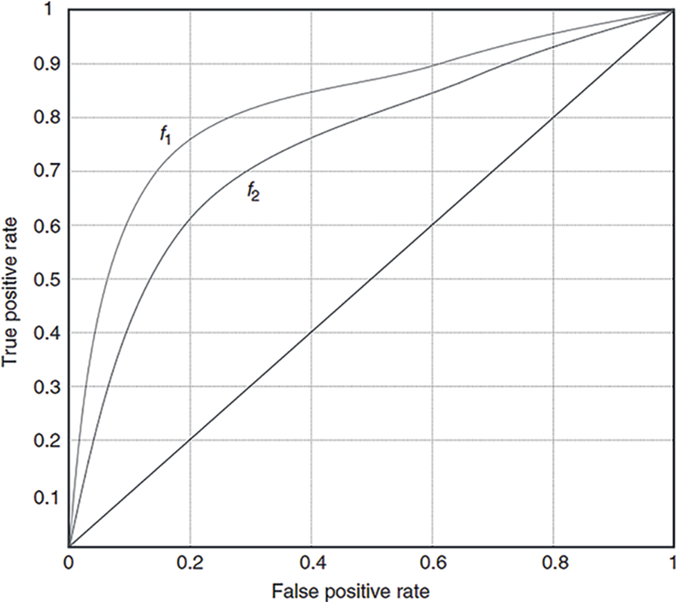
Figure 3: ROC curves for two hypothetical classifiers

4  Results and Discussion

4.1 Feature Importance

In this study, RFE, SHAP, and Shap-Hypetune algorithms were used on the dataset to calculate feature importance. Using RFE with Decision trees resulted in eliminating five features (N, HER2, Mets at Distant LN, ICD_O_2 Histology, and Laterality), while using the same algorithm with random forest classifier resulted in eliminating one feature only (Laterality). Shapely values along with Shap-hypetune were used on XGBoost model to calculate feature importance, this resulted in excluding one feature only (ICD_O_2 Histology). Finally, the CatBoost built-in feature importance method was used to calculate feature importance, M and Laterality were the least important features. Fig. 4 shows an overview of feature importance for the four models.

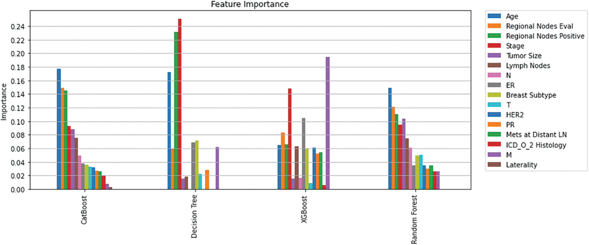
Figure 4: Feature importance per model

Understanding model decisions is essential for evaluating prediction consistency and spotting potential causes of model bias. SHAP’s objective is to compute the contribution of each feature to the prediction of an instance x to explain it. Shapley values are calculated using the SHAP explanation technique based on coalitional game theory. Fig. 5 shows how each feature is contributing to the prediction of each of the classes in CatBoost model. (Figs. 6–13) show the impact of each feature on the prediction of each class, values on the right side of the axis support the prediction positively, while values on the left side have a negative effect on the prediction. This is consistent with research results from the medical field, where factors like the age, lymph nodes, stage, tumour size, information on ER, PR, and HER2 play an important role in deciding which treatment(s) is to be considered [35,38,42,43].

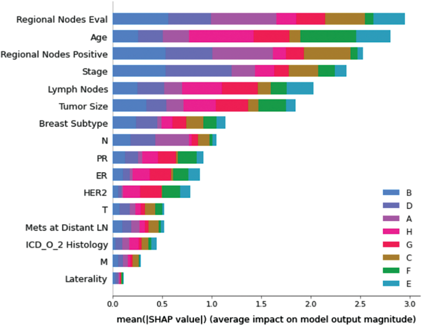
Figure 5: Mean SHAP values

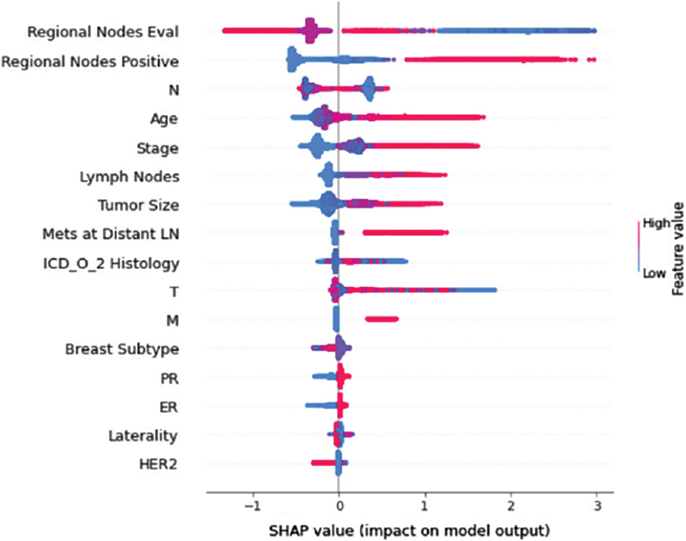
Figure 6: Class A-impact on model output

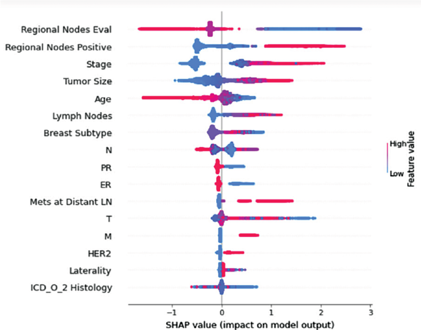
Figure 7: Class B-impact on model output

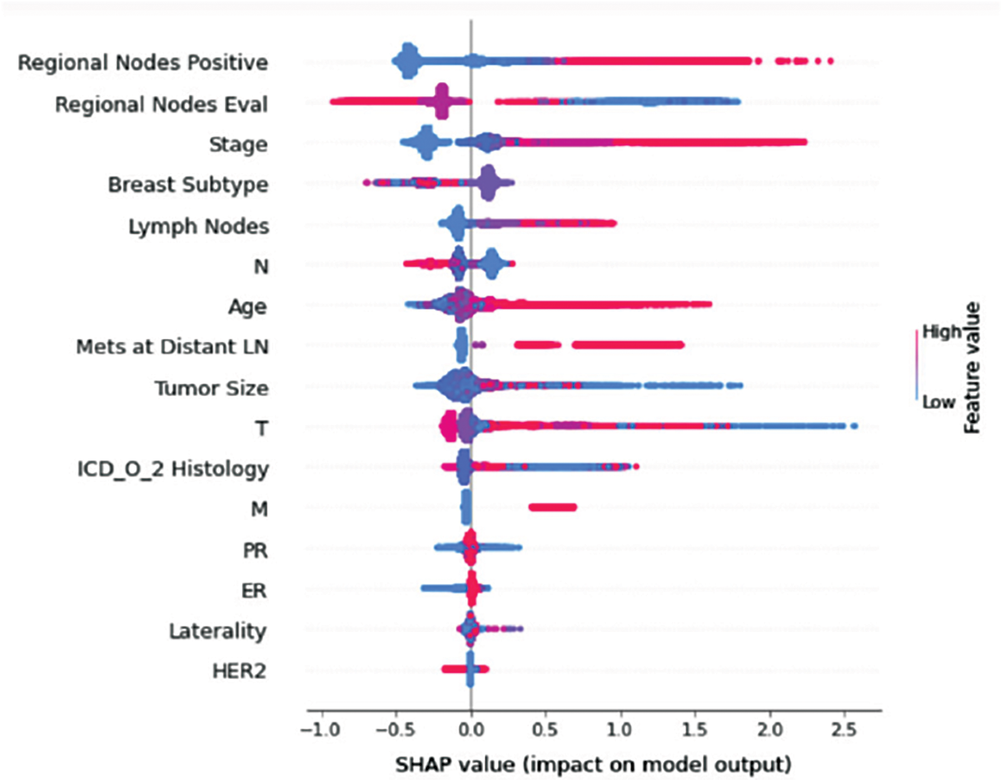
Figure 8: Class C-impact on model output

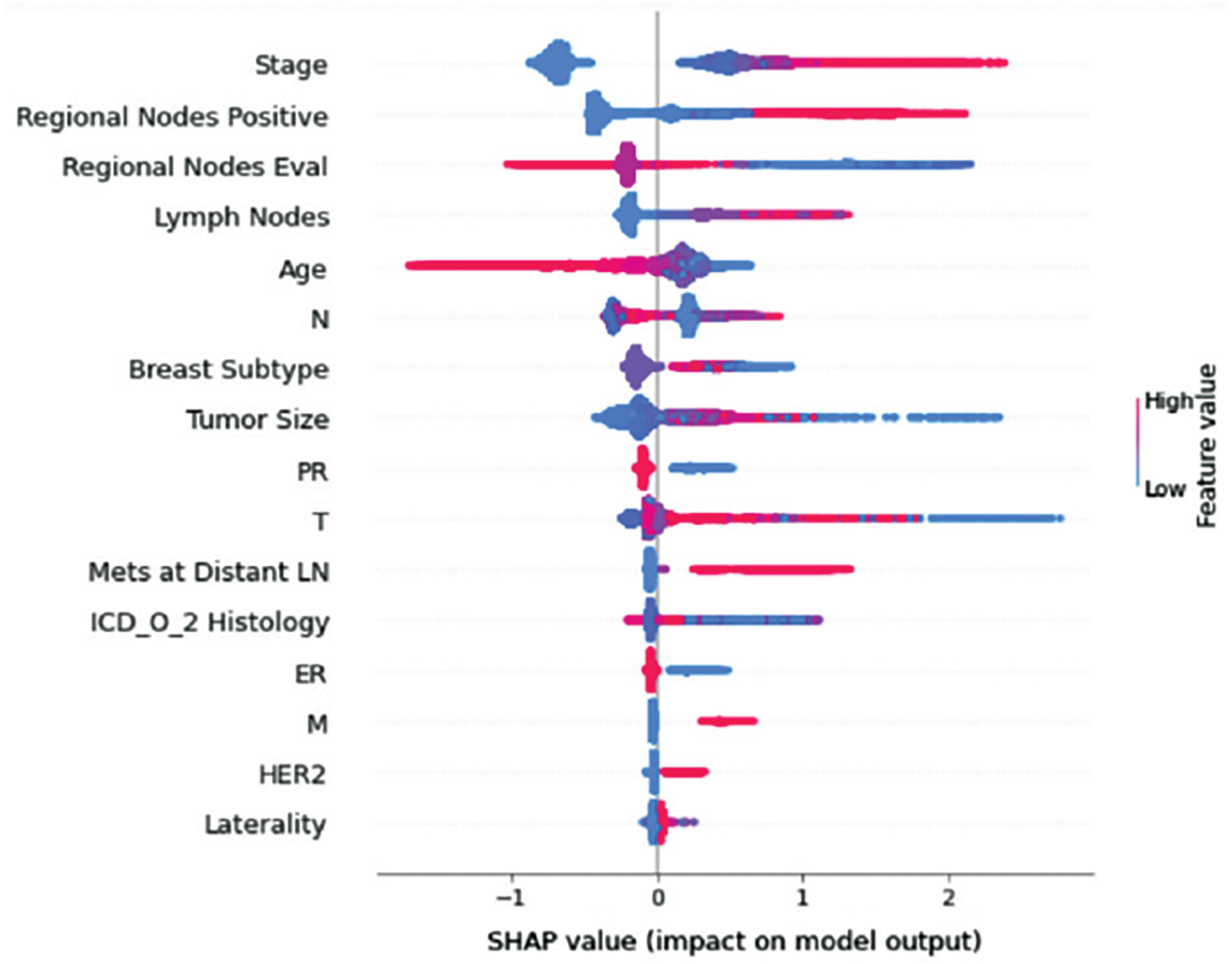
Figure 9: Class D-impact on model output

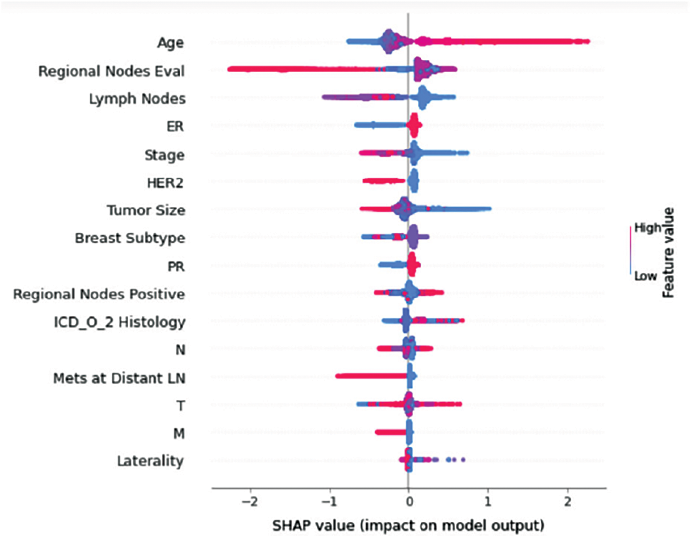
Figure 10: Class E-impact on model output

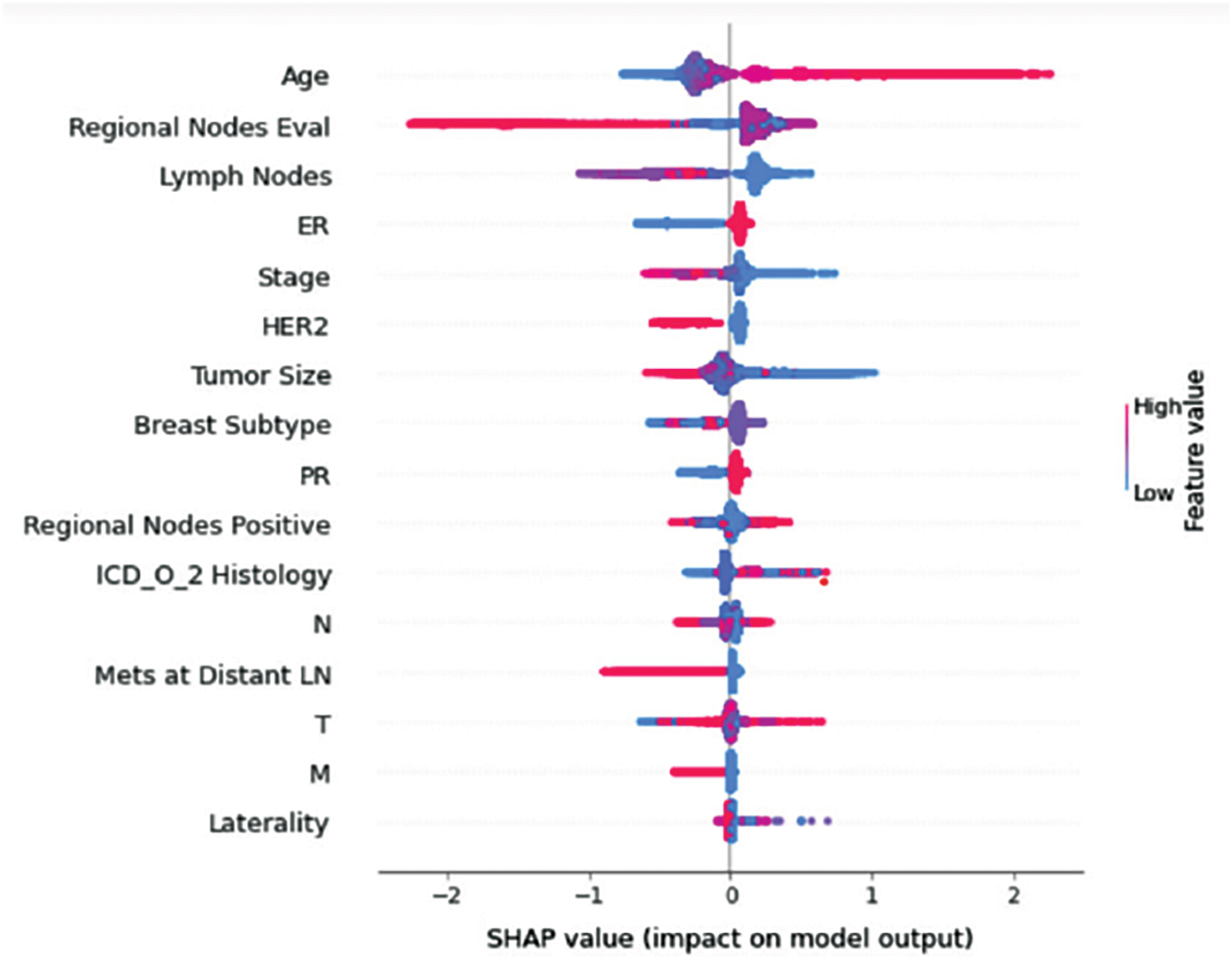
Figure 11: Class F-impact on model output

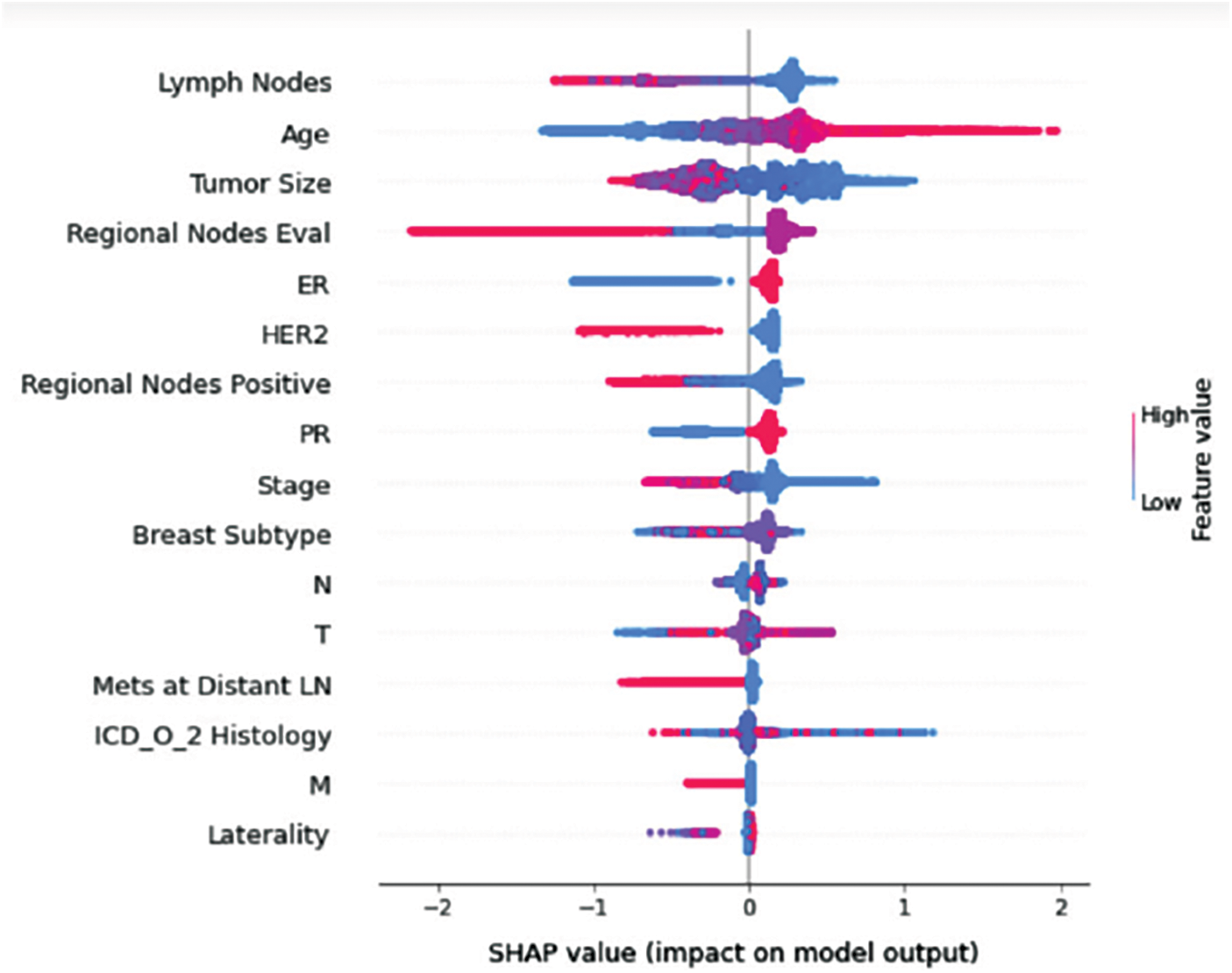
Figure 12: Class G-impact on model output

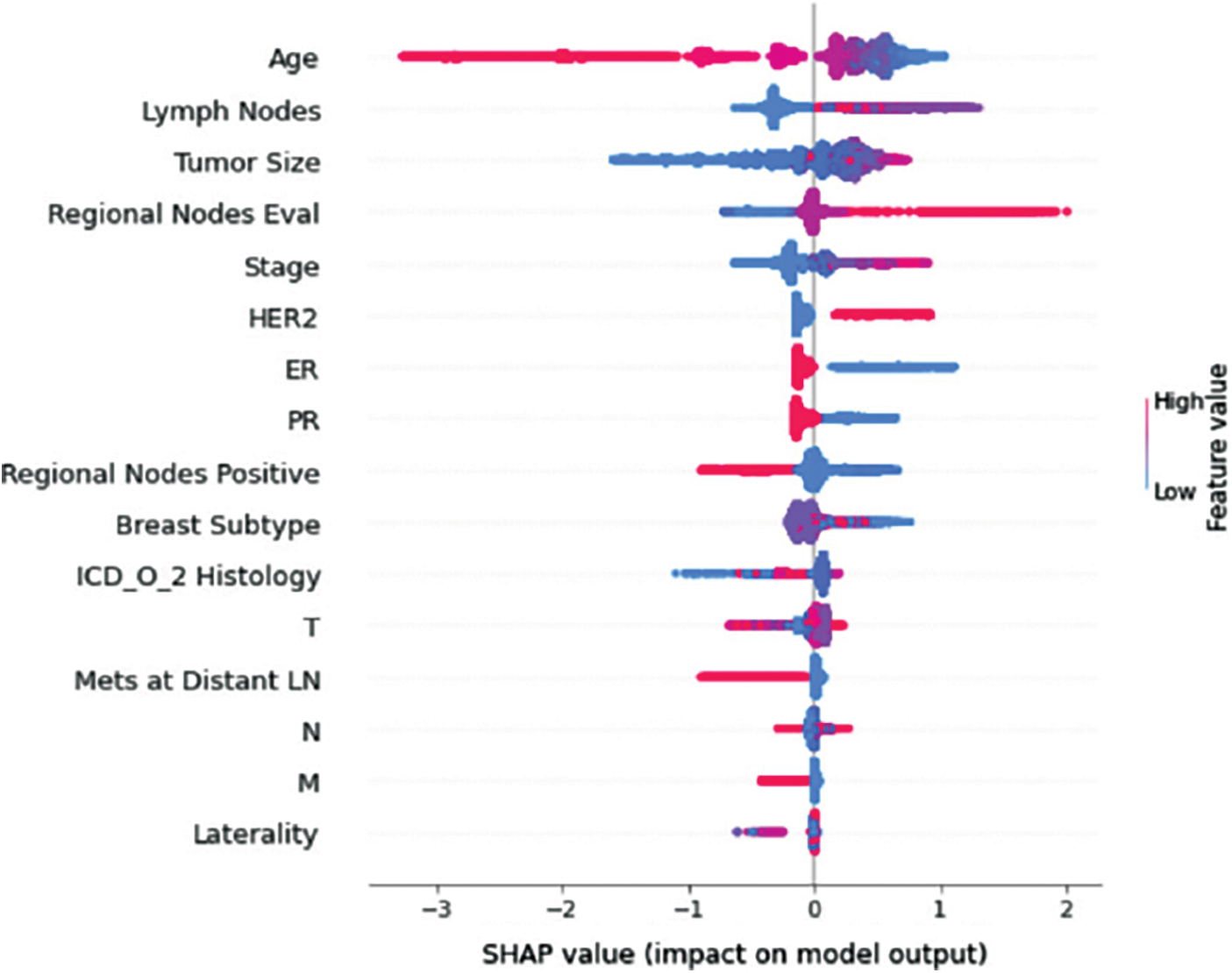
Figure 13: Class H-impact on model output

4.2 Classification Results

This study applied machine learning algorithms including Decision Trees, Random Forest, XGBoost, and CatBoost to predict a treatment plan using the SEER dataset, which includes sixteen features. After cleaning the data, the dataset was split into a training set and a validation set, and the models were fit on the training dataset containing 16 features. With five folds of stratified sampling inside each class, K-fold cross-validation was utilized to measure prediction error while maintaining the overall class distribution. AUC was used to evaluate the performance of the classifier. AUC for each class and the overall model AUC among different models were compared; Fig. 14 shows an overview of the achieved AUC per model per class. As can be seen, Random Forest performed better (overall AUC of 0.91) than the other models, which resulted in AUC of 0.88, 0.89, and 0.89 for Decision Trees, XGBoost, and CatBoost, respectively. AUC per class for the Random Forest model was superior to all the other models, where the model achieved an AUC of 0.98, 0.99, 0.99, 0.99, 0.78, 0.85, 0.84, and 0.88 for treatment classes A, B, C, D, E, F, G, and H respectively.

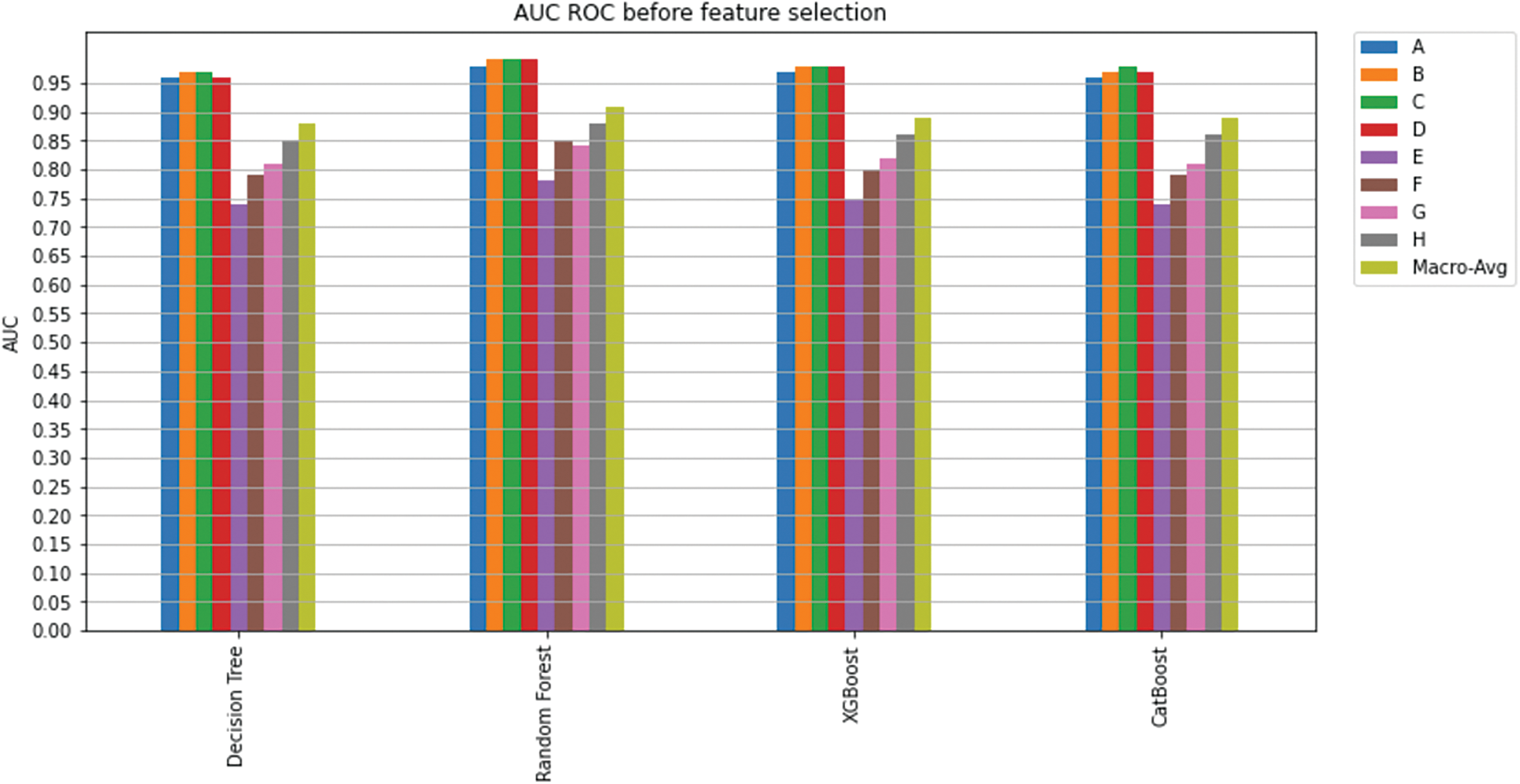
Figure 14: AUC ROC before feature selection

In the second phase, feature selection algorithms were utilized on the classification models, and the least important features were excluded (as explained in Section 5.1.1). K-fold cross-validation (K = 5) was used to measure model prediction; Fig. 15 shows an overview of the achieved AUC per model per class. There is no significant improvement for the overall model’s AUC or the AUC for each class. Yet again, Random Forest was superior to all the other classifiers and has shown excellent performance in predicting a treatment plan; indeed, it achieved an overall AUC of 0.91.

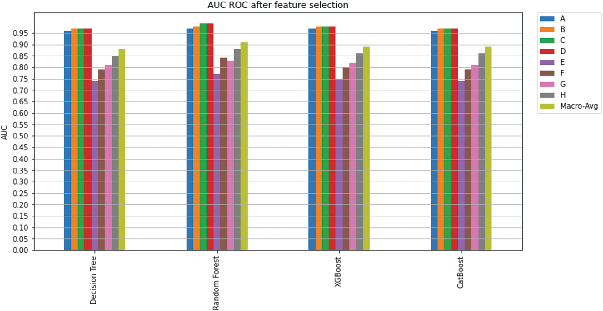
Figure 15: AUC ROC after feature selection

Considering both phases, we aimed to build a model that can successfully predict a treatment plan; we chose the best available features to support prediction. As can be seen, the best achieved AUC was 0.91 for the Random Forest model, which is considered a good result. However, we still have a low AUC for treatment classes E, F, G, and H. These classes correspond to a treatment plan where surgery and other treatments are recommended. Having a close look at the shapely summary plot for these classes (Figs. 10–13), one can see that the selected features are not supporting the model prediction for these classes. The high values of features like Regional Nodes Eval, Regional Nodes positive, and Mets at Distant LN negatively impact the prediction, especially for class E (AUC 0.78), which is the treatment plan that recommends surgery only.

5  Conclusion

In this paper, we have investigated the issue of breast cancer treatment plan prediction using four well-known classifiers, i.e., Decision Trees, Random Forest, XGBoost, and CatBoost. These classifiers were utilized with the SEER dataset, which contains sixteen features. The best overall AUC achieved was 0.91 for the Random Forest classifier.

Feature importance, especially shapely summary plots, provided informative information on the contribution of each of the selected features to the model prediction. It gives physicians a valuable hint to pay greater attention to these critical aspects when diagnosing clinical breast tumours. With the reduced number of features, Random Forest achieved the best overall AUC (0.91) across the other classifiers. Feature importance also revealed some possible reasons for the low performance of the selected models in predicting classes that include surgery as part of the treatment plan. One could investigate this further and try to find other features that would improve the performance of these models.

The study suggested a Random Forest model that may be further developed as a potential practical methodology for a CDS system to propose a breast cancer treatment plan by providing physicians with a second opinion. Such a CDS system can also help inexperienced physicians to avoid suggesting the wrong treatment plan.

Funding Statement: N.I.R.R. and K.I.M. have received a grant from the Malaysian Ministry of Higher Education. Grant number: 203/PKOMP/6712025; http://portal.mygrants.gov.my/main.php.

Conflicts of Interest: The authors declare that they have no conflicts of interest to report regarding the present study.

References

1. B. Anderson, Breast cancer, WHO, 2022. [Online]. Available: https://www.who.int/news-room/fact-sheets/detail/breast-cancer. [Google Scholar]

2. F. Winsberg, M. Elkin, J. Macy, V. Bordaz and W. Weymouth, “Detection of radiographic abnormalities in mammograms by means of optical scanning and computer analysis,” Radiology, vol. 89, no. 2, pp. 211–215, 1967. [Google Scholar]

3. M. D. Dorrius, M. C. Jansen-Van Der Weide, P. M. A. Van Ooijen, R. M. Pijnappel and M. Oudkerk, “Computer-aided detection in breast MRI: A systematic review and meta-analysis,” European Radiology, vol. 21, no. 8, pp. 1600–1608, 2011. [Google Scholar] [PubMed]

4. A. Jalalian, S. B. T. Mashohor, H. R. Mahmud, M. I. B. Saripan, A. R. B. Ramli et al., “Computer-aided detection/diagnosis of breast cancer in mammography and ultrasound: A review,” Clinical Imaging, vol. 37, no. 3, pp. 420–426, 2013. [Google Scholar] [PubMed]

5. S. M. Friedewald, E. A. Rafferty, S. L. Rose, M. A. Durand, D. M. Plecha et al., “Breast cancer screening using tomosynthesis in combination with digital mammography,” JAMA-Journal of the American Medical Association, vol. 311, no. 24, pp. 2499–2507, 2014. [Google Scholar]

6. M. L. Giger, “Machine learning in medical imaging,” Journal of the American College of Radiology, vol. 15, no. 3, pp. 512–520, 2018. [Google Scholar] [PubMed]

7. D. Sheth and M. L. Giger, “Artificial intelligence in the interpretation of breast cancer on MRI,” Journal of Magnetic Resonance Imaging, vol. 51, no. 5, pp. 1310–1324, 2020. [Google Scholar] [PubMed]

8. I. Abdel-Qader and F. Abu-Amara, “A computer-aided diagnosis system for breast cancer using independent component analysis and fuzzy classifier,” Modelling and Simulation in Engineering, vol. 2008, no. 4, pp. 1–9, 2008. [Google Scholar]

9. D. Newell, K. Nie, J. H. Chen, C. C. Hsu, H. J. Yu et al., “Selection of diagnostic features on breast MRI to differentiate between malignant and benign lesions using computer-aided diagnosis: Differences in lesions presenting as mass and non-mass-like enhancement,” European Radiology, vol. 20, no. 4, pp. 771–781, 2010. [Google Scholar] [PubMed]

10. C. Gallego-Ortiz and A. L. Martel, “Improving the accuracy of computer-aided diagnosis for breast MR imaging by differentiating between mass and nonmass lesions,” Radiology, vol. 278, no. 3, pp. 679–688, 2016. [Google Scholar] [PubMed]

11. US food and drug administration, Premarket Approval (PMA), 2021. [Online]. Available: https://www.accessdata.fda.gov/scripts/cdrh/cfdocs/cfpma/pma.cfm?ID=319829. [Google Scholar]

12. R. L. Birdwell, D. M. Ikeda, K. F. O’Shaughnessy and E. A. Sickles, “Mammographic characteristics of 115 missed cancers later detected with screening mammography and the potential utility of computer-aided detection,” Radiology, vol. 219, no. 1, pp. 192–202, 2001. [Google Scholar] [PubMed]

13. T. W. Freer and M. J. Ulissey, “Screening mammography with computer-aided detection: Prospective study of 12,860 patients in a community breast center,” Radiology, vol. 220, no. 3, pp. 781–786, 2001. [Google Scholar] [PubMed]

14. J. D. Keen, J. M. Keen and J. E. Keen, “Utilization of computer-aided detection for digital screening mammography in the United States, 2008 to 2016,” Journal of the American College of Radiology, vol. 15, no. 1, pp. 44–48, 2018. [Google Scholar] [PubMed]

15. C. D. Lehman, R. D. Wellman, D. S. M. Buist, K. Kerlikowske, A. N. A. Tosteson et al., “Diagnostic accuracy of digital screening mammography with and without computer-aided detection,” JAMA Internal Medicine, vol. 175, no. 11, pp. 1828–1837, 2015. [Google Scholar] [PubMed]

16. M. U. Rehman, S. Najm, S. Khalid, A. Shafique, F. Alqahtani et al., “Infrared sensing based non-invasive initial diagnosis of chronic liver disease using ensemble learning,” IEEE Sensors Journal, vol. 21, no. 17, pp. 19395–19406, 2021. [Google Scholar]

17. M. U. Rehman, A. Shafique, S. Khalid, M. Driss and S. Rubaiee, “Future forecasting of COVID-19: A supervised learning approach,” Sensors (Basel), vol. 21, no. 10, pp. 3322, 2021. [Google Scholar] [PubMed]

18. M. Bouchahma, S. ben Hammouda, S. Kouki, M. Alshemaili and K. Samara, “An automatic dental decay treatment prediction using a deep convolutional neural network on x-ray images,” in Proc. IEEE/ACS 16th Int. Conf. on Computer Systems and Applications (AICCSA), Abu Dhabi, UAE, pp. 1–4, 2019. [Google Scholar]

19. I. Christoyianni, A. Koutras, E. Dermatas and G. Kokkinakis, “Computer aided diagnosis of breast cancer in digitized mammograms,” Computerized Medical Imaging and Graphics, vol. 26, no. 5, pp. 309–319, 2002. [Google Scholar] [PubMed]

20. L. Tsochatzidis, L. Costaridou and I. Pratikakis, “Deep learning for breast cancer diagnosis from mammograms-A comparative study,” Journal of Imaging, vol. 5, no. 3, pp. 37, 2019. [Google Scholar] [PubMed]

21. A. Berlin, M. Sorani and I. Sim, “A taxonomic description of computer-based clinical decision support systems,” Journal of Biomedical Informatics, vol. 39, no. 6, pp. 656–667, 2006. [Google Scholar] [PubMed]

22. A. D. Seidman, M. L. Pilewskie, M. E. Robson, J. F. Kelvin, M. G. Zauderer et al., “Integration of multi-modality treatment planning for early-stage breast cancer (BC) into Watson for oncology, a decision support system: Seeing the forest and the trees,” Journal of Clinical Oncology, vol. 33, no. 15_suppl, pp. e12042, 2015. [Google Scholar]

23. Z. Jie, Z. Zhiying and L. Li, “A meta-analysis of watson for oncology in clinical application,” Scientific Reports, vol. 11, no. 1, pp. 7, 2021. [Google Scholar]

24. V. Patkar, D. Acosta, T. Davidson, A. Jones, J. Fox et al., “Cancer multidisciplinary team meetings: Evidence, challenges, and the role of clinical decision support technology,” International Journal of Breast Cancer, vol. 2011, pp. 1–7, 2011. [Google Scholar]

25. T. J. Bright, A. Wong, R. Dhurjati, E. Bristow, L. Bastian et al., “Effect of clinical decision-support systems a systematic review,” Annals of Internal Medicine, vol. 157, no. 1, pp. 29–43, 2012. [Google Scholar] [PubMed]

26. S. B. Holmes, J. L. B. Carter and A. Metefa, “Lesson of the week: Blunt orbital trauma,” British Medical Journal, vol. 321, no. 7263, pp. 750–751, 2000. [Google Scholar] [PubMed]

27. Breast cancer organization, What is breast cancer?, 2020. [Online]. Available: https://www.breastcancer.org/symptoms/understand_bc/what_is_bc. [Google Scholar]

28. Centers for disease control and prevention, What is breast cancer?, 2021. [Online]. Available: https://www.cdc.gov/cancer/breast/basic_info/what-is-breast-cancer.htm. [Google Scholar]

29. S. M. Swain, J. Baselga, S. B. Kim, J. Ro, V. Semiglazov et al., “Pertuzumab, Trastuzumab, and Docetaxel in HER2-positive metastatic breast cancer,” New England Journal of Medicine, vol. 372, no. 8, pp. 724–734, 2015. [Google Scholar] [PubMed]

30. A. G. Waks and E. P. Winer, “Breast cancer treatment: A review,” JAMA Journal of the American Medical Association, vol. 321, no. 3, pp. 288–300, 2019. [Google Scholar] [PubMed]

31. S. B. Edge and C. C. Compton, “The american joint committee on cancer: The 7th edition of the AJCC cancer staging manual and the future of TNM,” Annals of Surgical Oncology, vol. 17, no. 6, pp. 1471–1474, 2010. [Google Scholar] [PubMed]

32. A. Bardia, I. A. Mayer, J. R. Diamond, R. L. Moroose, S. J. Isakoff et al., “Efficacy & safety of anti-Trop-2 antibody drug conjugate Sacituzumab govitecan (IMMU-132) in heavily pre-treated patients with metastatic triple-negative breast cancer,” Journal of Clinical Oncology, vol. 35, no. 19, pp. 2141–2148, 2017. [Google Scholar] [PubMed]

33. National cancer institute, Breast cancer treatment (Adult), 2021. [Online]. Available: https://www.cancer.gov/types/breast/patient/breast-treatment-pdq#_185. [Google Scholar]

34. H. Barghava, Breast cancer: Symptoms, Risk Factors, Diagnosis, Treatment & Prevention, Webmd, 2020. [Online]. Available: https://www.webmd.com/breast-cancer/understanding-breast-cancer-basics. [Google Scholar]

35. Association of Breast Surgery at Baso 2009, “Surgical guidelines for the management of breast cancer,” European Journal of Surgical Oncology (EJSO), vol. 35, pp. S1–S22, 2009. [Google Scholar]

36. S. Møller, M. B. Jensen, B. Ejlertsen, K. D. Bjerre, M. Larsen et al., “The clinical database and the treatment guidelines of the danish breast cancer cooperative group (DBCG); Its 30-years experience and future promise,” Acta Oncologica, vol. 47, no. 4, pp. 506–524, 2008. [Google Scholar]

37. E. Senkus, S. Kyriakides, S. Ohno, F. Penault-Llorca, P. Poortmans et al., “Primary breast cancer: ESMO clinical practice guidelines for diagnosis, treatment and follow-up,” Annals of Oncology, vol. 26, no. Supplement 5, pp. v8–v30, 2015. [Google Scholar] [PubMed]

38. B. Fisher, S. Anderson, J. Bryant, R. G. Margolese, M. Deutsch et al., “Twenty-year follow-up of a randomized trial comparing total mastectomy, lumpectomy, and lumpectomy plus irradiation for the treatment of invasive breast cancer,” New England Journal of Medicine, vol. 347, no. 16, pp. 1233–1241, 2002. [Google Scholar] [PubMed]

39. P. McGale, C. Taylor, C. Correa, D. Cutter, F. Duane et al., “Effect of radiotherapy after mastectomy and axillary surgery on 10-year recurrence and 20-year breast cancer mortality: Meta-analysis of individual patient data for 8135 women in 22 randomised trials,” The Lancet, vol. 383, no. 9935, pp. 2127–2135, 2014. [Google Scholar]

40. National cancer institute, “SEER explorer application,” 2021. [Online]. Available: https://seer.cancer.gov/explorer/application.html?site=55&data_type=1&graph_type=4&compareBy=sex&chk_sex_3=3&chk_sex_2=2&race=1&age_range=1&advopt_precision=1&advopt_display=2. [Google Scholar]

41. C. Bernard-Marty, F. Cardoso and M. J. Piccart, “Facts and controversies in systemic treatment of metastatic breast cancer,” The Oncologist, vol. 9, no. 6, pp. 617–632, 2004. [Google Scholar] [PubMed]

42. F. Cardoso, P. L. Bedard, E. P. Winer, O. Pagani, E. Senkus-Konefka et al., “International guidelines for management of metastatic breast cancer: Combination vs sequential single-agent chemotherapy,” J Natl Cancer Inst, vol. 101, no. 17, pp. 1174–1181, 2009. [Google Scholar] [PubMed]

43. E. Breast, C. Trialists and C. Group, “Adjuvant chemotherapy in oestrogen-receptor-poor breast cancer: Patient-level meta-analysis of randomised trials,” The Lancet, vol. 371, no. 9606, pp. 29–40, 2008. [Google Scholar]

44. J. M. Lebert, R. Lester, E. Powell, M. Seal and J. McCarthy, “Advances in the systemic treatment of triple-negative breast cancer,” Current Oncology, vol. 25, no. June, pp. S142–S150, 2018. [Google Scholar] [PubMed]

45. “Surveillance, epidemiology, and end results program,” National cancer institute, 2021. [Online]. Available: https://seer.cancer.gov/. [Google Scholar]

46. “Female breast cancer—cancer stat facts,” National cancer institute, 2022. [Online]. Available: https://seer.cancer.gov/statfacts/html/breast.html. [Google Scholar]

47. J. Li, K. Cheng, S. Wang, F. Morstatter, R. P. Trevino et al., “Feature selection: A data perspective,” ACM Computing Surveys, vol. 50, no. 6, pp. 1–45, 2017. [Google Scholar]

48. J. Cai, J. Luo, S. Wang and S. Yang, “Feature selection in machine learning: A new perspective,” Neurocomputing, vol. 300, pp. 70–79, 2018. [Google Scholar]

49. G. Chandrashekar and F. Sahin, “A survey on feature selection methods,” Computers and Electrical Engineering, vol. 40, no. 1, pp. 16–28, 2014. [Google Scholar]

50. I. Jain, V. K. Jain and R. Jain, “Correlation feature selection based improved-binary particle swarm optimization for gene selection and cancer classification,” Applied Soft Computing, vol. 62, no. 16, pp. 203–215, 2018. [Google Scholar]

51. D. Mishra and B. Sahu, “Feature selection for cancer classification: A signal-to-noise ratio approach,” International Journal of Scientific & Engineering Research, vol. 2, no. 4, pp. 1–7, 2011. [Google Scholar]

52. C. Nguyen, Y. Wang and H. N. Nguyen, “Random forest classifier combined with feature selection for breast cancer diagnosis and prognostic,” Journal of Biomedical Science and Engineering, vol. 6, no. 5, pp. 551–560, 2013. [Google Scholar]

53. sklearn.feature_selection.RFE—scikit-learn 1.0.2 documentation,” Scikit learn, 2022. [Online]. Available: https://scikit-learn.org/stable/modules/generated/sklearn.feature_selection.RFE.html. [Google Scholar]

54. P. M. Granitto, C. Furlanello, F. Biasioli and F. Gasperi, “Recursive feature elimination with random forest for PTR-MS analysis of agroindustrial products,” Chemometrics and Intelligent Laboratory Systems, vol. 83, no. 2, pp. 83–90, 2006. [Google Scholar]

55. B. H. Young, “Monotonic solutions of cooperative games x,” International Journal of Game Theory, vol. 14, pp. 65–72, 1985. [Google Scholar]

56. I. Kumar, S. Venkatasubramanian, C. Scheidegger and S. Friedler, “Problems with Shapley-value-based explanations as feature importance measures,” in Proc. Int. Conf. on Machine Learning, Virtual, pp. 5491–5500, 2020. [Google Scholar]

57. M. Cerliani, “Shap-hypetune,” PyPi, 2022. [Online]. Available: https://pypi.org/project/shap-hypetune/. [Google Scholar]

58. S. B. Kotsiantis, “Decision trees: A recent overview,” Artificial Intelligence Review, vol. 39, no. 4, pp. 261–283, 2013. [Google Scholar]

59. C. Kingsford and S. L. Salzberg, “What are decision trees?,” Nature Biotechnology, vol. 26, no. 9, pp. 1011–1013, 2008. [Google Scholar] [PubMed]

60. L. Breiman, J. H. Friedman, R. A. Olshen and C. J. Stone, “Classification and regression trees,” in Classification and Regression Trees, 1st ed., Routledge, pp. 1–358, 2017. [Google Scholar]

61. L. Breiman, “Random forests,” Machine Learning, vol. 45, no. 1, pp. 5–32, 2001. [Google Scholar]

62. J. Friedman, T. Hastie and R. Tibshirani, “Additive logistic regression: A statistical view of boosting,” The Annals of Statistics, vol. 28, no. 2, pp. 337–407, 2000. [Google Scholar]

63. XGBoost Documentation—xgboost 1.5.2 documentation, XGBoost, 2021. [Online]. Available: https://xgboost.readthedocs.io/en/stable/. [Google Scholar]

64. T. Chen and C. Guestrin, “XGBoost: A scalable tree boosting system,” in Proc. of the ACM SIGKDD Int. Conf. on Knowledge Discovery and Data Mining, San Francisco California, pp. 785–794, 2016. [Google Scholar]

65. T. Chen and T. He, “XGBoost: eXtreme gradient boosting,”. 2017. [Online]. Available: https://cran.microsoft.com/snapshot/2017-12-11/web/packages/xgboost/vignettes/xgboost.pdf. [Google Scholar]

66. A. Gulin, “CatBoost-open-source gradient boosting library,” Catboost, 2022. [Online]. Available: https://catboost.ai/. [Google Scholar]

67. A. V. Dorogush, V. Ershov and A. G. Yandex, “CatBoost: Gradient boosting with categorical features support,” arXiv Preprint. arXiv:1810.11363, 2008. [Google Scholar]

68. L. Prokhorenkova, G. Gusev, A. Vorobev, A. V. Dorogush and A. Gulin, “CatBoost: Unbiased boosting with categorical features,” in Proc. 32nd Conf. on Neural Information Processing Systems (NeurIPS 2018), Monetreal, Canada, 2018. [Google Scholar]

69. N. Japkowicz, “8 assessment metrics for imbalanced learning,” in Imbalanced Learning: Foundations, Algorithms, and Applications, 1st ed., Wiley-IEEE press, Hoboken, New Jersey, pp. 187–206, 2013. [Google Scholar]

70. Y. Sun, A. K. C. Wong and M. S. Kamel, “Classification of imbalanced data: A review,” International Journal of Pattern Recognition and Artificial Intelligence, vol. 23, no. 4, pp. 687–719, 2009. [Google Scholar]

71. A. N. Tarekegn, M. Giacobini and K. Michalak, “A review of methods for imbalanced multi-label classification,” Pattern Recognition, vol. 118, Elsevier Ltd., pp. 107965, 2021. [Google Scholar]

72. M. Grandini, E. Bagli and G. Visani, “Metrics for multi-class classification: An overview,” arXiv Preprint. arXiv:2008.05756, 2020. [Google Scholar]