Hyperparameter Tuning for Deep Neural Networks Based Optimization Algorithm

1  Introduction

It will speed up the review and typesetting process. Neural Networks (NNs) are models with successive layers of neurons that have been in existence for decades. Training for these NNs can be done either in an unsupervised or supervised manner. The most frequently used machine learning technique for either shallow or deep networks is supervised learning Soydaner [1]. This technique will calculate an objective function that measures the error or distance between the actual result and the expected result. The learning procedure will involve adapting its internal parameters such that this error is minimized. The term “weights” is employed for these adjustable parameters. Deep Neural Networks (DNNs) are made up of millions of weights that may require to be updated during the training procedure.

The DNN model Shin et al., [2] will constitute a nested architecture of layers in which the number of parameters is in millions. The deep model’s high degrees of freedom will enable it to be approximate non-linear as well as linear functions; despite that, this model is constantly at the risk of overfitting to training data. The deep neural network will require regularization techniques in the training procedure so as to accomplish generalization, and hence, yield good predictions for the unknown data.

When training DNNs, it is generally beneficial to decrease the Learning Rate (LR) Yedida et al., [3] with the progression of the training. This is done by employing pre-defined LR schedules or adaptive LR methods. LR schedules will try to adjust the LR during the training procedure by mitigating the LR as per a pre-defined schedule. Exponential decay, step decay, and time-based decay are the well-known LR schedules.

The choice of algorithm for a NN’s Yang et al., [4] optimization is one of the most critical steps. Machine learning has three key types of optimization methods. The first type is referred to as batch or deterministic gradient methods. These methods will simultaneously process all the training examples in a large batch. The second type is known as the stochastic or online methods, which will only utilize a single example at a time. Nowadays, the majority of the algorithms are a combination of the two afore-mentioned types of methods. These algorithms are termed mini-batch methods as, during the training procedure, they utilize only a part of the training set at each epoch. In the era of Deep Learning (DL) era, mini-batch methods are chiefly preferred for two key reasons. Firstly, these methods can accelerate the NNs’ training. Secondly, there will be computation of the expected gradient’s unbiased estimate since the mini-batches are chosen at random and are independent.

Investigation of the hyperparameter search space generally needs huge number of epochs for training the model with unique settings of the hyperparameters Wu et al., [5]. In consequence, to naively run the model to retrieve optimized hyperparameters will need a remarkably vast number of GPUs, and it will be vital to search the hyperparameter in the search space in most efficient manner. The work of hyperparameter optimization is to train the target deep learning model various number of times, each time with an unlike configuration and assess it every time. Every sub procedure during training period is recognized by the model’s exclusive configuration. The training of contemporary DL models in order to attain highly advanced accuracy will necessitate the alteration of hyperparameter values during the training process since the objective is the minimization of high dimensional and non-convex loss functions. Therefore, a single or set of hyperparameter configuration is treated as a value or array of values, which has examples like network architecture parameters, input sequence length, training image input size, image augmentation parameters, batch size, momentum, optimizer, drop-out ratio, and LR.

Dropout is a principle in which some of the neurons are not considered in the training process. These randomly selected neurons are dropped out. That is, during the forward pass the role of the activation of downstream neurons is removed temporarily. The same way during the backward pass, updation of weights is not implemented to the selected neuron. This reduces the time for the whole training process.

Notwithstanding its popularity, the training of NNs is rife with numerous problems Alyafi et al., [6], such as over-fitting, exploding gradient, and vanishing gradient. These problems can be resolved with various advances inclusive of different activation functions, batch normalization, novel initialization schemes, and dropout. Nevertheless, a more elemental problem involves the detection of optimal values for the numerous hyper-parameters, of which the most vital one is the LR. It is a widely known fact that exceedingly small LR has slow convergence while huge LR can result in divergence. It has been noted in recent works that, instead of a fixed value of LR, a non-monotonic LR scheduling system will offer quicker convergence.

Optimizing the structure of the network and loss function is a NP (nondeterministic polynomial time) hard process Vasudevan [7]. For enhancing the models’ generalization capabilities, different network structures have been designed for application in diverse scenarios. Thus, manually designed network structures are generally highly targeted. In accordance with different tasks, it is generally necessary to redesign or optimize the network structure deeply in order to maintain the generalization performance in the new scenarios, which in turn consumes a huge amount of manpower as well as computing resources.

Effective hyperparameter selection would result in earlier convergence to the global minimum point on the error surface. This results in improved task performance while still avoiding issues such as overfitting. In this work, it is proposed to optimize the set of hyperparameters (Learning rate, Activation Function, Dropout) for RNNs, LSTM and BiLSTM by using the Adaptive Teaching Learning Based Optimization (ATLBO) algorithm. The rest of this investigation has been organized into the following sections. Section two details the related works in literature. Section three elaborates on the various methods employed in this work. Section four describes the experimental outcomes, and Section five gives the work’s conclusions.

2  Related Works

Chen et al., [8] had presented a broad study of thirteen Learning Rate functions as well as their associated Learning Rate policies by analyzing their range value, step value, and value update parameters. The authors had suggested a metric set for the assessment and selection of Learning Rate (LR) policies, inclusive of robustness, cost, variance, and classification confidence, and had set them in a Learning Rate Benchmarking system known as the Learning Rate Bench. The LR Bench would aid DNN developers as well as end-users to pick a suitable Learning rate policies and also to avoid unsuitable Learning Rate policies so as to train their DNNs. The authors had gauged the LR Bench on Caffe, an open-source deep learning framework, for demonstrating the tuning and optimization of Learning Rate policies. By means of comprehensive experimentations and its assessments, this work attempted to clarify the fine-tuning of LR policies by detecting appropriate policies with effectual range of LR values together with step sizes for the Learning Rate schedulers.

Fischetti et al., [9] had put forward a powerful technique to pick an LR range for a neural network named CLR (Contaminated Land Report) with two distinct skewness. This proposed technique would adjust where the value is cycled between a lower bound and an upper bound. Simplistic in computation, the CLR policies could avoid the computational expense of fine tuning with fixed LR. It was quite evident that altering the LR during the training phase had offered more superior results in comparison to fixed values with the same or even smaller number of epochs.

Li et al. [10] had given the demonstration of a novel approach to training DNNs through the use of a Mutual Information (MI)-driven, decaying LR, Stochastic Gradient Descent (SGD) algorithm. For every epoch of the training cycle, the MI amidst the neural network output and exact fallout was used to strongly set the Learning Rate for the deep neural network. Since the MI instinctively offered a layer-wise attainment metric, this opinion was stretched-out to a layer-wise fixing of the Learning rate. Proposal for an LR range test to determine the operating LR range was also given. Experiments were done to draw a comparison between this approach and other well-known alternatives like gradient-based adaptive LR algorithms such as Adam, RMSprop, and LARS (Laboratory Assistant and Research Systems). Competitive to better accuracy outcomes which were attained in competitive to a better time, had demonstrated the feasibility of the metric as well as the proposed approach.

Yang et al. [11] had devised a Decaying Momentum (DEMON) rule, which was motivated by decaying a gradient’s total contribution to all future updates. The application of DEMON to Adam will result in substantially improved training, which is remarkably competitive to momentum SGD with LR decay, even in settings where the adaptive methods are normally non-competitive. Likewise, the application of DEMON to momentum SGD will rival momentum SGD with LR decay, and in certain cases, will result in improved performance. In comparison to the vanilla counterparts, DEMON has simple implementation and also has limited extra computational overhead.

Liu et al. [12] had proposed a novel meta-heuristic training scheme that unconventionally combined SGD and discrete optimization. The scheme defines a separate neighbourhood of the current SGD point, which was made up of number of “probably good moves” which could accomplish gradient information, and to pursuit this neighbourhood through the use of a standard meta-heuristic scheme which had been borrowed from discrete optimization. The authors had examined the usage of a simple Simulated Annealing (SA) meta-heuristic which could accept/reject a candidate new solution in the neighbourhood with a probability that was dependent on both the new solution quality and on a parameter (temperature) that was modified over time so as to minimize the probability of accepting worsening moves. This work’s title originated from how this scheme was utilized as an automated way to carry out hyper-parameter tuning. A unique feature of this scheme was that hyper-parameters were modified within a single SGD execution (rather than in an external loop, as per custom) and assessed on the fly on the current mini-batch; that is, their tuning was fully embedded inside the SGD algorithm.

Smith [13] had modeled the SGD-induced training trajectory via a feasible Stochastic Differential Equation (SDE) that had a noise term that could capture the gradient noise. This, in turn, yields: (a) A new “intrinsic LR” parameter which was the product of the normal LR η and the weight decay factor λ. The SDE analysis showed how the learning’s effective speed would vary and equilibrate overtime under the intrinsic LR’s control. (b) A challenge—via theory and experimentations—to popular belief that good generalization needed huge LRs at the training’s start. (c) New experimentations, supported by mathematical intuition, suggested that the number of steps to equilibrium (in function space) would scale as the intrinsic LR’s inverse, as opposed to the exponential time convergence bound that had been implied by the SDE analysis.

Hsueh et al., [14] had devised a new LR schedule known as Piecewise Arc Cotangent decay Learning rate (PACL), that could enhance the DNN’s accuracy as well as convergence speed and also could substantially mitigate the performance degradation zone caused by the cycling mechanism. The PACL had the ease of implementation and had almost no extra computing expense. Eventually, this work had demonstrated the PACL’s effectiveness in training CIFAR-10, CIFAR-100, and Tiny ImageNet with ResNet, DenseNet, WRN, SEResNet, and MobileNet.

Literature survey based on NNs, DNNs, decaying LRs, optimizing hyperparameters for deep learning used in various domains are presented here. The observation from the surveys, they have concentrated only on anyone of the Hyperparameter in the model to achieve better accuracy. Especially the learning rate is decayed by using various methods (CLR, HTD and T-HTR) Yu et al., [15]. However, one drawback is that it does not consider a set of hyperparameters, which affects the rate of convergence of the network on the error surface. Through this survey the decision of considering proposed method techniques to enhance the existing results was taken.

3  Learning Rates

3.1 Cyclical Learning Rates (CLR)

This Learning Rate policy’s essence comes from the observation that even though increasing the LR may have a short-term negative effect; it can accomplish a more long-term beneficial effect. In view of this observation, the concept would be to allow the LR to vary within a range of values instead of adopting a value that is either stepwise fixed or exponentially decreasing. That is, the minimum and maximum boundaries will be set, and the learning rate will cyclically vary between these bounds Apaydin et al., [16]. Equivalent results were produced by experimentations with multiple functional forms like a triangular window (linear), a Welch window (parabolic), and a Hann window (sinusoidal). This resulted in the adoption of a triangular window (which will linearly increase and then linearly decrease), since it is the simplest function that incorporates the above-mentioned concept.

With due consideration to the loss function topology, it is possible to achieve an intuitive understanding of the CLR methods’ operating principles. Dauphin et al., had debated that the difficulty in minimizing the loss emerged from the saddle points instead of the poor local minima. Saddle points have small gradients, which slow down the learning procedure. Nevertheless, the learning rate could be increased to allow for a swifter traversal of the saddle point plateaus. In all likelihood, the optimum learning rate would be between the bounds, and the near-optimal learning rates would be utilized throughout the training. For the CLR’s optimization, the root means the square error was employed as the fitness. The ATLBO algorithm was used to detect the optimal learning rate.

3.2 Hyperbolic-Tangent Decay (HTD) Scheduler

This work had proposed a new LR scheduler referred to as the Hyperbolic-Tangent decay (HTD) scheduler. When compared with the step decay scheduler, the HTD was found to have fewer hyperparameters to tune and also showed better performance in all the experimentations. On the other hand, when compared with the cosine scheduler, the HTD needed slightly more hyperparameters to tune for higher performance and also exceeded the performance of cosine schedulers Chen et al., [17].

This work will propose to utilize hyperbolic tangent functions for the Learning Rate scheduling as per the below Eq. (1):

lrtHTD =lrmin+lrmax−lrmin2(1−tanh(L(1−tT)+UtT))  (1)

Here, lrmax will indicate the maximum LR, lrmin will indicate the minimum Learning Rate (LR), T will indicate the total number of epochs (or iterations), 0 ≤ t ≤ T will indicate the index of epoch (or iteration), while L and U will indicate the lower and upper bounds of the interval [L, U] for the function tanh x.

In HTD (L, U), the hyperparameters U will affect the final learning rate. As an example, when U = 3, the final learning rate will be lrmax . (1 − tanh 3) ≈  lrmax · 0.005. Moreover, it is able to adjust the lower bound L to alter the ratio, R = |L|/|U|, which is the ratio of the training times before and after the inflection point. The ATLBO algorithm is used to find the optimal values for L and U.

3.3 Toggle Between Hyperbolic Tangent Decay and Triangular Mode with Restarts (T-HTR) Learning Rate Scheduler

The T-HTR’s concept is to flip the Learning Rate scheduler’s hyperbolic tangent decay and triangular mode amongst the iterations in the batches of the epoch. This will reduce the training time’s length and also enhance the model’s learning. The earlier epochs’ specifics (like epoch number, learning rate and gradient value) can be used to decide on the LR scheduler of the next epoch’s initial iterations. An average of all the batches’ LR is taken. This average will be utilized as the next epoch’s initial Learning Rate. The ATLBO algorithm is used to find the optimal learning rate at the earliest.

3.4 Teaching Learning Based Optimization (TLBO) Algorithm

All of the evolutionary- and swarm intelligence-based algorithms are probabilistic algorithms and require common controlling parameters, like the population size, number of generations, elite size, etc. In addition to the common control parameters, algorithm-specific control-parameters are required. For example, Genetic Algorithm (GA) uses the mutation rate and crossover rate. Similarly, Particle Swarm Optimization (PSO) uses the inertia weight, as well as social and cognitive parameters. The proper tuning of algorithm-specific parameters is a very crucial factor that, affects the performance of the above-mentioned algorithms. The improper tuning of algorithm-specific parameters either increases the computational effort or yields a local optimal solution. Therefore, introduced the TLBO algorithm, which requires only the common control parameters and does not require any algorithm-specific control parameters. Other evolutionary algorithms require the control of common control parameters as well as the control of algorithm-specific parameters. The burden of tuning common control parameters is comparatively less in the TLBO algorithm. Based upon the above discussion, TLBO algorithm steps are Rao et al., [18,19].

Step 1: The optimization parameters are set with initial values

•   Size of the population

•   Number of iterations

•   Number of subjects (decision variables)

Step 2: The random population is created based on the size of the population and the number of design variables.

Step 3: The fitness of the potential solutions are evaluated and the population is organized based on their fitness value.

Step 4: Teacher Phase: The mean of the population is calculated. This provides the mean of the particular subject.

Step 5: Learner Phase: The solution is simulated by: learners gain knowledge by mutually interacting among themselves.

Step 6: From step 3, it is repeated till the stopping criteria is met.

Step 7: Stop the process.

Thus, the TLBO algorithm is simple, effective and involves comparatively less computational effort. The ATLBO algorithm is the improved form of TLBO (Chen et al. 2018) algorithm to make it more effective in finding the optimized values for the hyperparameters in the model.

4  Methodology

4.1 Adaptive Teaching Learning Based Optimization (ATLBO)

Teaching-learning is a critical process in which each individual would attempt to learn something from the other individuals so as to improve them. This algorithm sought to replicate a classroom’s conventional teaching-learning phenomenon by simulating two fundamental learning modes: (i) through the teacher (termed the teacher phase) and (ii) through interactions with other learners (termed the learner phase). Being a population-based algorithm, the ATLBO would consider a group of students (that is, the learner) as the population, and the different subjects who were provided to the learners would be akin to the optimization problem’s different design variables. The learner’s results would be analogous to the optimization problem’s value of fitness. The teacher would be the whole population’s best solution. Below is the explanation of the ATLBO algorithm’s operation with the teacher phase as well as the learner phase Wang et al. [20].

4.2 Teacher Phase

This algorithm phase would simulate the students’ (that is, the learners) learning through the teacher. During this phase, a teacher would convey knowledge amongst the learners and would try to raise the class’s mean result. Consider that ‘m’ number of subjects (that is, design variables) were given to ‘n’ number of learners (that is, size of the population, k = 1, 2 . . . n). At any sequential teaching-learning cycle i, Mj,i would be the learners’ mean result in a certain subject ‘j’ (j = 1, 2 . . . m). A teacher would be a subject’s most experienced and knowledgeable person. Hence, the teacher in the algorithm would be the best learner in the whole population. Suppose that Xtotal−kbest,i would be the result of the best learner considering all the subjects who have been identified as that cycle’s teacher. Even though the teacher would put maximum effort into increasing the entire class’s knowledge level, the learners would only gain knowledge in accordance with the quality of teaching delivered by a teacher as well as the class’s quality of learners present. In view of this fact, Eq. (2) would express the difference between the teacher’s result and the mean result of the learners in each subject as follows:

Difference_Meani,j=ri(Xj,kbest,i−TFMj,i) (2)

where, Xj,kbest,i will indicate the teacher’s (that is, the best learner) result in the subject j, TF will indicate the teaching factor, that determines the value of mean to be modified, and ri will indicate the random number in the range [0, 1]. The TF value can be either 1 or 2. The TF value will be randomly decided with equal probability as per below Eq. (3):

TF=round[1+rand(0, 1){2−1}]  (3)

where, the rand will indicate the random number in the range [0, 1]. TF will not be a parameter of the algorithm. The TF value will not be offered as the algorithm’s input. Instead, the algorithm will use Eq. (3) to randomly decide the TF value. Moreover, these parameters do not get offered as the algorithm’s input (which is contrary to the supply of the Genetic Algorithm’s (GA) crossover probability and mutation probability, the Particle Swarm Optimization (PSO’s) inertia colony size and limit, and so on). Therefore, the algorithm does not require the tuning of ri and TF (which is contrary to the tuning of the GA’s crossover probability and mutation probability, the PSO’s inertia weight and cognitive and social parameters, the ABC’s colony size and limit, and so on). For its operation, the ATLBO algorithm only needs to tune common control parameters such as the size of the population and the number of generations. These common control parameters are requisite for the operation of all population-based optimization algorithms. Therefore, the ATLBO is termed as an algorithm-specific parameter-less algorithm.

The algorithm’s performance is affected by the values of both ri and TF. The students’ understanding from best teacher may be dissimilar and arbitrary. The learning of students from teacher is uncertain some times when the teaching factor in Eq. (3) is used. So, Information entropy is used to capture the extent of diversion of student’s performance. When the entropy is low, the diversion is high. In this stage, the teaching factor should be high to lower the search ability. When the entropy is high and dispersion is minimum means, then the performance is normal. The Probability Distribution (PD) for the performance of the student is

PD(xj,i)=xj,i∑j−1m⁡xj,i (4)

The entropy for the particular subject i is:

Subi=−∑j=1m⁡PD(xj,i)logPD(xj,i) (5)

TFi=TFu−(TFu−TFlSubu)∗Subi (6)

where l is lower bound and u is upper bound and TFi is new Teaching factor based on entropy. The diversion of the students’ performance is reduced which improves the learning process in the teacher’s phase. In ATLBO algorithm the new teaching factor TFi Eq. (6) is used as an alternative of TF .

Based on the Difference_Meanj,i , update of the existing solution in the teacher phase will be in accordance with the below Eq. (7):

Xj,k,i′=Xj,k,i+Difference_Meanj,i (7)

This equation Xj,k,i′ will indicate the updated value of Xj,k,i . Xj,k,i′ is accepted if it is able to offer a better function value. All the accepted function values at the teacher phase’s end will be maintained, and in turn, these values will become the learner phase’s input.

Learner phase: This algorithm phase will stimulate the students’ (that is, the learners) learning via interactions amongst themselves. In addition to that, the students can gain knowledge through discussion and interaction with other students. A learner is able to learn new information if the other learners have more knowledge than him or her. Below is the explanation of this phase’s learning phenomenon.

There is a random selection of two learners, P and Q, such that Xtotal−P.i′≠Xtotal−Q.i′ , where, Xtotal−P.i′ and Xtotal−Q.i′ will be the updated values of Xtotal−P.i and Xtotal−Q.i , respectively, at the teacher phase’s end in Eqs. (8) and (9):

Xj,P.i′′=Xj,P.i′+ri(Xj,P.i′−Xj,Q.i′ ),  IfXtotal−P.i′ > Xtotal−Q.i′ (8)

Xj,P.i′′=Xj,P.i′+ri(Xj,Q.i′− Xj,Q.i′)IfXtotal−Q.i′ > Xtotal−P.i′  (9)

(While the above equations are for maximization problems, the reverse will be true for minimization problems) Xj,P.i″ . It is accepted if it is able to offer a better function value.

The optimization of hyperparameters (learning rate and dropout) for RNN, LSTM and BiLSTM models is attained through the teacher phase and learner phase of the ATLBO Algorithm. It is used for the classification problem. The steps are given below.

Step 1: Initialize the population size, number of decision variables and Termination criterion

Step 2: Evaluate the mean of each decision variable

Step 3: Estimate the Fitness value

Step 4: Select the individual with best fitness as teacher

Step 5: Implement the teacher phase and Learner phase of ATLBO algorithm

Step 6: Get the optimal values for the hyperparameters learning rate and dropout of the Model

Step 7: Train the RNN/LSTM/BiLSTM Model with the optimal hyperparameters

Step 8: Test the model with the optimal hyperparameter values

Step 9: Find the Accuracy/Error

Step 10: End

The teacher and Learner phase is repeated many times till the stopping criterion is met. The stopping criterion is the maximum number of iterations considered in the ATLBO algorithm. At the end, the optimal hyperparameters learning rate for the learning rate scheduler and dropout is obtained. This optimal learning rate is used in the learning rate schedulers CLR, HTD and T-HTR.

The learning rate schedulers and dropout are utilized in the RNN, LSTM and BiLSTM models for the training process. The model is trained and tested on the datasets 20Newsgroup, ReutersNewswire and IMDB. The classification accuracy accomplished for the models using ATLBO algorithm is recorded in the Tables 1–3.

The same way the optimal hyperparameter got using TLBO algorithm is given as input to the model. It is trained and tested on the datasets 20Newsgroup, Reutersnewswire and IMDB. The classification accuracy attained for the models using TLBO algorithm is documented in the Tables 1–3. The accuracy attained using ATLBO algorithm is compared with accuracy attained using TLBO algorithm. The ATLBO algorithm performs better than the TLBO algorithm in all the cases. BiLSTM T-HTR scheduler performs better than the other schedulers using ATLBO algorithm.

Classification accuracy statistic by itself will not determine which learning model is the best. There are several measures for evaluating the performance of various models with specified optimal features, such as Precision, Recall, and F-Measure.

5  Results and Discussions

In this section, the 20Newsgroup, Reuters Newswire and IMDB movie reviews datasets are evaluated. The features are extracted using TF_IDF. The RNN CLR, RNN HTD, RNN T-HTR, LSTM CLR, LSTM HTD, LSTM T-HTR, BiLSTM CLR, BiLSTM HTD and Bi LSTM T-HTR methods [18–20] are used. The precision, recall and f-measure are shown in Tables 4–6. The comparisons are shown Figs. 1–3.

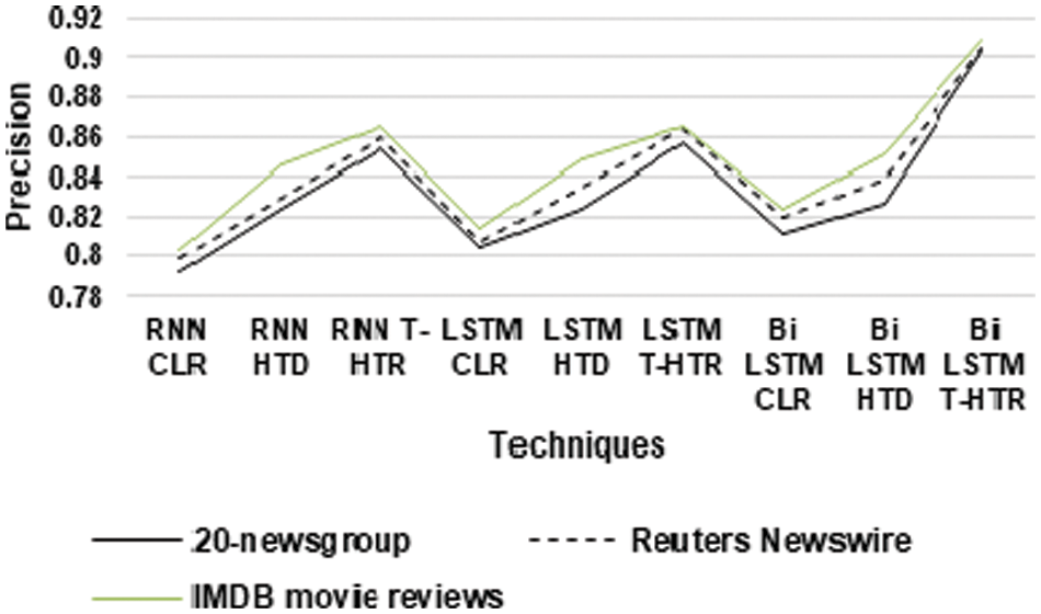
Figure 1: Precision for ATLBO algorithm

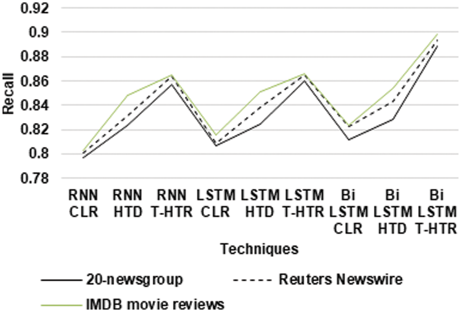
Figure 2: Recall for ATLBO algorithm

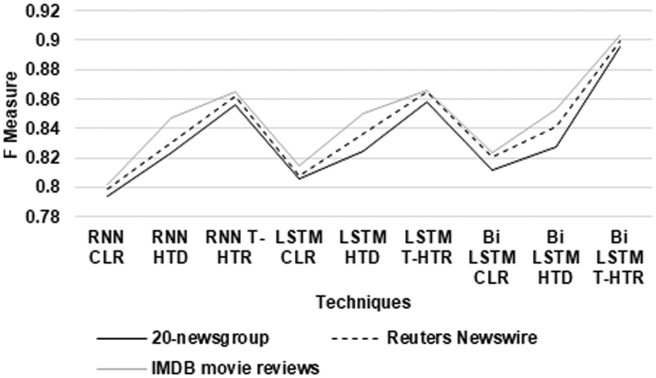
Figure 3: F-Measure for ATLBO algorithm

From Fig. 1, it can be observed that the BiLSTM T-HTR has higher precision for 20-newsgroup datasets by 13.19% for RNN CLR, by 9.26% for RNN HTD, by 5.56% for RNN T-HTR, by 11.61% for LSTM CLR, by 9.25% for LSTM HTD, by 5.36% for LSTM T-HTR, by 10.76% for BiLSTM CLR and by 9.02% for BiLSTM HTD respectively. The Bi LSTM T-HTR has higher precision for Reuters Newswire datasets by 12.55% for RNN CLR, by 8.7% for RNN HTD, by 5.06% for RNN T-HTR, by 11.51% for LSTM CLR, by 8.13% for LSTM HTD, by 4.58% for LSTM T-HTR, by 9.93% for BiLSTM CLR and by 7.56% for Bi LSTM HTD respectively. The BiLSTM T-HTR has higher precision for IMDB movie reviews datasets by 12.48% for RNN CLR, by 7.23% for RNN HTD, by 4.94% for RNN T-HTR, by 11.08% for LSTM CLR, by 6.84% for LSTM HTD, by 4.9% for LSTM T-HTR, by 9.86% for BiLSTM CLR and by 6.45% for BiLSTM HTD respectively.

From the Fig. 2, it can be observed that the Bi LSTM T-HTR has higher recall for 20-newsgroup datasets by 10.87% for RNN CLR, by 7.49% for RNN HTD, by 3.61% for RNN T-HTR, by 9.64% for LSTM CLR, by 7.4% for LSTM HTD, by 3.18% for LSTM T-HTR, by 8.97% for BiLSTM CLR and by 6.95% for BiLSTM HTD respectively. The BiLSTM T-HTR has higher recall for Reuters Newswire datasets by 10.93% for RNN CLR, by 7.19% for RNN HTD, by 3.26% for RNN T-HTR, by 9.86% for LSTM CLR, by 6.3% for LSTM HTD, by 3.19% for LSTM T-HTR, by 8.24% for BiLSTM CLR and by 5.76% for BiLSTM HTD respectively. The BiLSTM T-HTR has higher recall for IMDB movie reviews datasets by 11.22% for RNN CLR, by 5.65% for RNN HTD, by 3.71% for RNN T-HTR, by 9.64% for LSTM CLR, by 5.39% for LSTM HTD, by 3.63% for LSTM T-HTR, by 8.62% for BiLSTM CLR and by 5.02% for BiLSTM HTD respectively.

From Fig. 3, it can be observed that the BiLSTM T-HTR has a higher f measure for 20-newsgroup datasets by 12.03% for RNN CLR, by 8.38% for RNN HTD, by 4.58% for RNN T-HTR, by 10.62% for LSTM CLR, by 8.32% for LSTM HTD, by 4.27% for LSTM T-HTR, by 9.87% for Bi LSTM CLR and by 7.98% for BiLSTM HTD respectively. The BiLSTM T-HTR has a higher f-measure for Reuters Newswire datasets by 11.74% for RNN CLR, by 7.94% for RNN HTD, by 4.17% for RNN T-HTR, by 10.68% for LSTM CLR, by 7.21% for LSTM HTD, by 3.89% for LSTM T-HTR, by 9.08% for BiLSTM CLR and by 6.65% for BiLSTM HTD respectively. The BiLSTM T-HTR has a higher f-measure for IMDB movie reviews datasets by 11.85% for RNN CLR, by 6.44% for RNN HTD, by 4.33% for RNN T-HTR, by 10.37% for LSTM CLR, by 6.12% for LSTM HTD, by 4.27% for LSTM T-HTR, by 9.24% for BiLSTM CLR and by 5.74% for BiLSTM HTD respectively.

When ATLBO algorithm is used, the average training time of the RNN, LSTM and BiLSTM models on the three datasets is shown in the Tables 7 and 8 below. For 20Newsgroup dataset, the average training time has been decreased by 9.01% for RNN+T-HTR model, by 6.82% for LSTM+T-HTR, and by 7.80% for BiLSTM+T-HTR. In the similar manner, for Reuters Newswire and IMDB datasets, the average training time is reduced. The comparison of average training time for TLBO algorithm by considering the same models and datasets is shown in the Tables 7 and 8.

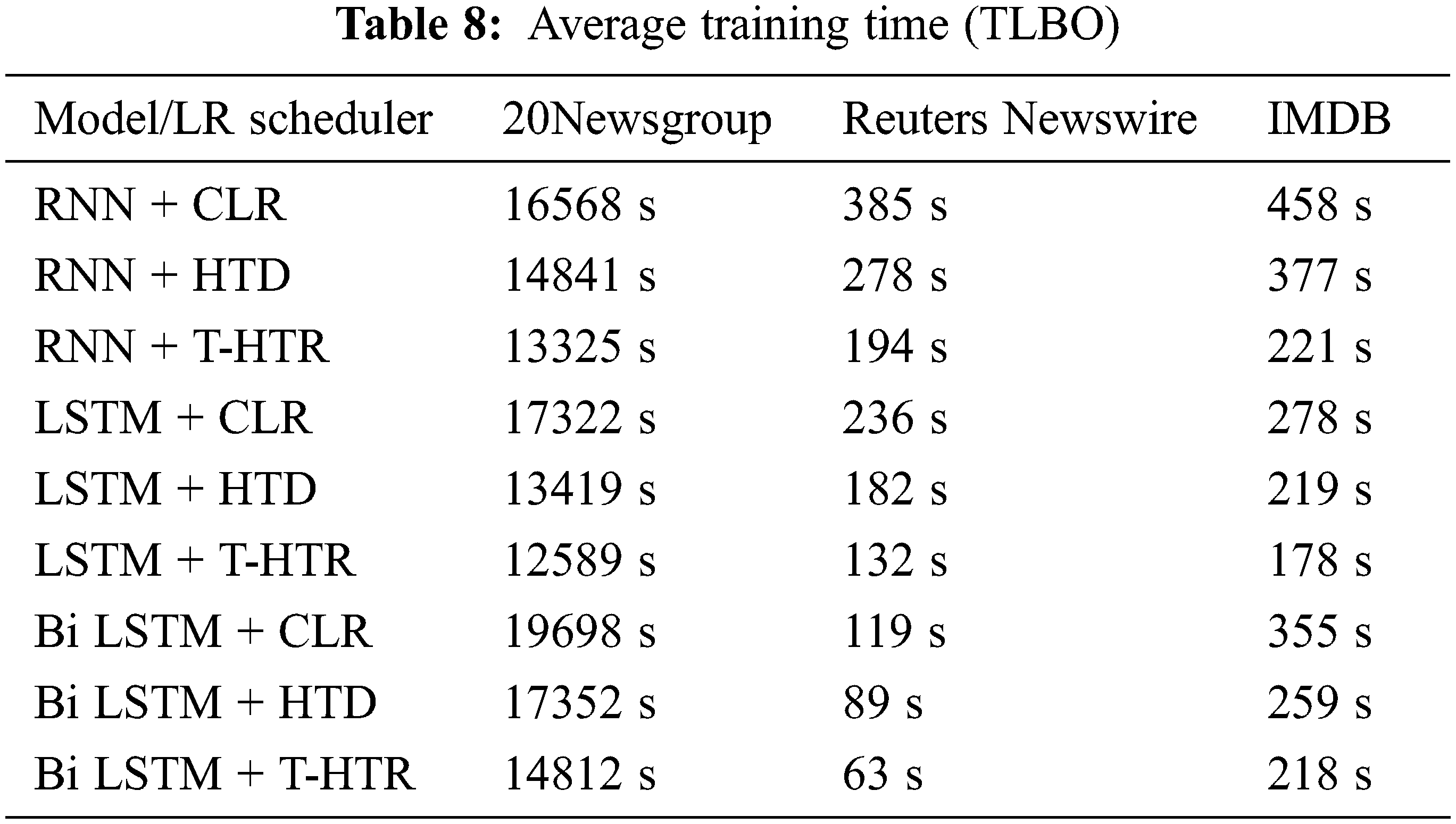
In all possible combinations, the ATLBO algorithm performs better. Also, it demonstrates that the BiLSTM+T-HTR has higher precision for 20Newsgroup, the Reuters Newswire datasets, and the IMDB movie reviews datasets in comparison to RNN CLR, RNN HTD, RNN T-HTR, LSTM CLR, LSTM HTD, LSTM T-HTR, BiLSTM CLR, and BiLSTM HTD. The average training time is also reduced much for BiLSTM T-HTR.

6  Conclusions

Optimization of DNNs is primarily accounted for as an empirical process that needs the manual tuning of various hyper-parameters like dropout rate, weight decay, and LR. Out of all these hyper-parameters, the LR is of prime importance and has been comprehensively researched in recent works. This work has given the proposal for a novel LR computation method to train DNNs with the ATLBO algorithm. The ATLBO algorithm’s application is done for the process of hyperparameter optimization. Inspired by the process of teaching–learning, this algorithm operates on the effect of a teacher’s influence on the output of learners in a class. The algorithm’s optimal hyperparameters is given as input for the RNN, LSTM and BiLSTM models The BiLSTM CLR is effective for quickly training a model and also has better accuracy in classification. When compared with the BiLSTM CLR, the BiLSTM HTD has superior performance in all the experimentations and also has fewer hyperparameters to tune. When compared with the BiLSTM HTD, the BiLSTM T-HTR has better performance in almost all the cases and also has more flexibility to accomplish better performance. When compared to models using the TLBO algorithm, the average training time for models utilizing the ATLBO approach is very short, indicating that convergence occurs first. Other hyperparameters of the model can be investigated for optimization using the ATLBO algorithm in future work.

Funding Statement: The authors received no specific funding for this study.

Conflicts of Interest: The authors declare that they have no conflicts of interest to report regarding the present study.

References

1. D. Soydaner, “A comparison of optimization algorithms for deep learning,” International Journal of Pattern Recognition and Artificial Intelligence, vol. 34, no. 13, pp. 2052013, 2020. [Google Scholar]
2. A. Shin, D. J. Shin, S. Cho, D. Y. Kim, E. Jeong et al., “Stage-based hyper-parameter optimization for deep learning,” arXiv preprint arXiv: 1911.10504, 2019. [Google Scholar]
3. R. Yedida and S. Saha, “A novel adaptive learning rate scheduler for deep neural networks,” arXiv preprint arXiv: 1902.07399, 2019. [Google Scholar]
4. J. Yang and F. Wang, “Auto-ensemble: An adaptive learning rate scheduling based deep learning model ensembling,” IEEE Access, vol. 8, pp. 217499–217509, 2020. [Google Scholar]
5. Y. Wu, L. Liu, J. Bae, K. H. Chow, A. Iyengar et al., “Demystifying learning rate policies for high accuracy training of deep neural networks,” in Proc. 2019 IEEE Int. Conf. on Big Data (Big Data), Los Angeles, CA, pp. 1971–1980, 2019. [Google Scholar]
6. B. Alyafi, F. I. Tushar and Z. Toshpulatov, “Cyclical learning rates for training neural networks with unbalanced datasets,” JMD in Medical Image Analysis and Applications-Pattern Recognition Module, pp. 1–4, 2018. https://doi.org/10.13140/RG.2.2.28455.80806 [Google Scholar] [CrossRef]
7. S. Vasudevan, “Mutual information based learning rate decay for stochastic gradient descent training of deep neural networks,” Entropy, vol. 22, no. 5, 560, pp. 1–15, 2020. [Google Scholar]
8. J. Chen and A. Kyrillidis, “Decaying momentum helps neural network training,” arXiv preprint arXiv: 1910.04952, 2019. [Google Scholar]
9. M. Fischetti and M. Stringher, “Embedded hyper-parameter tuning by simulated annealing,” arXiv preprint arXiv: 1906.01504, 2019. [Google Scholar]
10. Z. Li, K. Lyu and S. Arora, “Reconciling modern deep learning with traditional optimization analyses: The intrinsic learning rate,” arXiv preprint arXiv: 2010.02916, 2020. [Google Scholar]
11. H. Yang, J. Liu, H. Sun and H. Zhang, “PACL: Piecewise Arc cotangent decay learning rate for deep neural network training,” IEEE Access, vol. 8, pp. 112805–112813, 2020. [Google Scholar]
12. P. Liu, X. Qiu and X. Huang, “Recurrent neural network for text classification with multi-task learning,” arXiv preprint arXiv: 1605.05101, 2016. [Google Scholar]
13. L. N. Smith, “Cyclical learning rates for training neural networks,” in Proc. 2017 IEEE Winter Conf. on Applications of Computer Vision (WACV), Santa Rosa, CA, pp. 464–472, 2017. [Google Scholar]
14. B. Y. Hsueh, W. Li and I. C. Wu, “Stochastic gradient descent with hyperbolic-tangent decay on classification,” in Proc. 2019 IEEE Winter Conf. on Applications of Computer Vision (WACV), Waikoloa, HI, USA, pp. 435–442, 2019. [Google Scholar]
15. C. Yu, X. Qi, H. Ma, X. He, C. Wang et al., “LLR: Learning learning rates by LSTM for training neural networks,” Neurocomputing, vol. 394, no. 4, pp. 41–50, 2020. [Google Scholar]
16. H. Apaydin, H. Feizi, M. T. Sattari, M. S. Colak, S. Shamshirband et al., “Comparative analysis of recurrent neural network architectures for reservoir inflow forecasting,” Water, vol. 12, no. 5, pp. 1500, 2020. [Google Scholar]
17. X. Chen, B. Xu, K. Yu and W. Du, “Teaching-learning-based optimization with learning enthusiasm mechanism and its application in chemical engineering,” Journal of Applied Mathematics, vol. 2018, no. 1806947, pp. 19, 2018. [Google Scholar]
18. R. V. Rao and V. Patel, “An improved teaching-learning-based optimization algorithm for solving unconstrained optimization problems,” Scientia Iranica, vol. 20, no. 3, pp. 710–720, 2013. [Google Scholar]
19. R. V. Rao, V. J. Savsani and D. P. Vakharia, “Teaching-learning-based optimization: A novel method for constrained mechanical design optimization problems,” Computer-Aided Design, vol. 43, no. 3, pp. 303–15, 2011. [Google Scholar]
20. K. L. Wang, H. B. Wang, L. X. Yu, X. Y. Ma and Y. S. Xue, “Towards teaching-learning based optimization algorithm for dealing with real-parameter optimization problems,” in Proc. 2nd Int. Conf. on Computer Science and Electronics Engineering (ICCSEE 2013), Paris, Atlantis Press, pp. 607–609, 2013. [Google Scholar]
Cite This Article
Copyright © 2023 The Author(s). Published by Tech Science Press.
This work is licensed under a Creative Commons Attribution 4.0 International License , which permits unrestricted use, distribution, and reproduction in any medium, provided the original work is properly cited.
Downloads
Citation Tools